2014
Some Bayesian and multivariate analysis methods
in statistical machine learning and applications
Wen Zhou
Iowa State University
Follow this and additional works at:
https://lib.dr.iastate.edu/etd
Part of the
Applied Mathematics Commons, and the
Statistics and Probability Commons
This Dissertation is brought to you for free and open access by the Iowa State University Capstones, Theses and Dissertations at Iowa State University Digital Repository. It has been accepted for inclusion in Graduate Theses and Dissertations by an authorized administrator of Iowa State University Digital Repository. For more information, please [email protected].
Recommended Citation
Zhou, Wen, "Some Bayesian and multivariate analysis methods in statistical machine learning and applications" (2014).Graduate Theses and Dissertations. 13816.
and applications
by
Wen Zhou
A dissertation submitted to the graduate faculty in partial fulfillment of the requirements for the degree of
DOCTOR OF PHILOSOPHY
Major: Statistics
Program of Study Committee: Stephen Vardeman, Co-major Professor
Huaiqing Wu, Co-major Professor John Jackman
Max Morris Daniel Nordman
Iowa State University Ames, Iowa
2014
DEDICATION
I would like to dedicate this dissertation to my parents Zhenli Zhou and Xinhua Ren, my wife Linxing Yao and my daughter Michelle Zhou, without whose love and support I would not have been able to complete this work. I would also like to thank my friends for their help during the writing of this work.
TABLE OF CONTENTS
LIST OF TABLES . . . vii
LIST OF FIGURES . . . ix ACKNOWLEDGEMENTS . . . xiii CHAPTER 1. INTRODUCTION . . . 1 1.1 Background . . . 1 1.2 Literature Review . . . 4 1.2.1 Adaptive MCMC . . . 4
1.2.2 Data clustering and the self-organizing map . . . 5
1.2.3 Dataset shift in classifications . . . 6
1.2.4 Statistical inference on differential equation parameters . . . 7
1.3 Thesis Organization . . . 8
References . . . 8
CHAPTER 2. A GEOMETRICALLY ADAPTIVE METROPOLIS-HASTINGS ALGORITHM WITH GAUSSIAN CALIBRATION . . . 16
2.1 Introduction . . . 17
2.2 The New Adaptive Metropolis-Hastings Algorithm . . . 18
2.2.1 Motivation for the algorithm . . . 18
2.2.2 A geometrically adaptive Metropolis-Hastings algorithm for Θ⊂R . . . 21
2.2.3 Extension of the algorithm to Θ⊂Rp withp >1 . . . . 23
2.3 Numerical Studies . . . 25
2.3.1 Simulation studies for Θ⊂R . . . 26
2.3.3 Nuclear pump failures example . . . 35
2.4 Convergence Results . . . 36
2.5 Conclusion . . . 41
2.6 Appendix: Covariance Matrix Σ for Target Distribution (2.3.2) . . . 41
References . . . 42
CHAPTER 3. A BAYESIAN HIERARCHICAL TOPOGRAPHIC CLUS-TERING METHOD MOTIVATED BY THE SELF-ORGANIZING MAP 44 3.1 Introduction . . . 45
3.1.1 Self-organizing maps (SOMs): an overview . . . 45
3.1.2 A probabilistic alternative: generative topographic mapping (GTM) . . 47
3.1.3 A Bayesian hierarchical topographic clustering (BHTC) method . . . . 49
3.1.4 Organization of the rest of the paper . . . 51
3.1.5 Notation . . . 52
3.2 More Details of the Bayesian Hierarchical Topographic Clustering Model . . . . 52
3.2.1 Latent grid labeling . . . 52
3.2.2 Prototype model . . . 53
3.2.3 Models for the covariance matrix components . . . 55
3.2.4 Hyperparameters . . . 58
3.3 Posterior Distributions and Gibbs Samplings . . . 60
3.3.1 The posterior distributions . . . 61
3.3.2 Gibbs algorithm . . . 64
3.4 Optimal BHTC Based on Posterior Risk Functions . . . 67
3.4.1 Risk functions of the Hamming type . . . 67
3.4.2 Penalty functions for topographic preservation . . . 68
3.4.3 Risk equivalence classes . . . 70
3.4.4 Optimal clustering rule . . . 71
3.5 The BHTC, Markov Random Field and SOM . . . 74
3.5.1 The BHTC and MRF . . . 74
3.6 Numerical Studies . . . 78
3.6.1 Descriptions of four data sets . . . 78
3.6.2 BHTC results . . . 80
3.6.3 Comparison with other clustering methods . . . 83
3.7 Conclusions and Discussions . . . 89
3.8 Appendix: Technical Details for Model Derivations . . . 92
3.8.1 Technical details for model derivations . . . 92
3.8.2 Some details about the Hoff sampler . . . 96
3.8.3 Proof of Proposition3.4.5 . . . 98
3.8.4 Proof of Theorem3.4.6 . . . 101
3.8.5 Technical details for Section 5 . . . 102
References . . . 103
CHAPTER 4. CLASSIFICATION BASED ON ACTIVE SET SELECTION 110 4.1 Introduction . . . 111
4.2 Methodology . . . 114
4.2.1 A motivating example . . . 115
4.2.2 Algorithm of the ASSC . . . 118
4.2.3 A preliminary screening step . . . 120
4.3 Numerical Studies . . . 123
4.3.1 Simulation . . . 123
4.3.2 Analysis of real data . . . 125
4.4 Theoretical Properties . . . 127
4.4.1 Properties of sampling probabilities forP . . . 128
4.4.2 Validity of preliminary marginal screening . . . 128
4.5 Conclusions and Discussions . . . 129
CHAPTER 5. A BAYESIAN ANALYSIS OF THE DYNAMICS
DUR-ING CO-INFECTION BYLEISHMANIA MAJORANDLEISHMANIA
AMAZONENSIS BASED ON DIFFERENTIAL EQUATION MODELS . 134
5.1 Introduction . . . 135
5.2 Background and Examination of the Data . . . 136
5.2.1 Immunobiological mechanism . . . 136
5.2.2 Description of the data . . . 137
5.2.3 Variability of the measured data . . . 138
5.3 Bayesian Models . . . 140
5.3.1 Data model . . . 140
5.3.2 Linking the data model to the DE model . . . 141
5.3.3 Process/DE model . . . 142
5.3.4 Parameter model . . . 143
5.3.5 Hierarchical model summary . . . 145
5.4 Results of Bayesian Modeling and Analysis . . . 146
5.4.1 Model comparison and selection . . . 146
5.4.2 Estimation and inferences concerning model parameters . . . 148
5.4.3 Data fitting and further exploration . . . 150
5.4.4 Immune efficiency . . . 153
5.5 Conclusion and Discussion . . . 155
References . . . 157
LIST OF TABLES
Table 2.1 Comparisons between Algorithm 2.2.1 with c2 = 1 and c2 = c2opt and standard MH algorithms with normal proposal distributions with
dif-ferent fixed variances based on 50,000 iterations. . . 29
Table 2.2 Comparisons between Algorithm 2.2.3 (with c2 = 1 or c2 = c2 opt) and standard normal MH algorithms with multivariate normal proposal dis-tributions with different fixed covariance matrices based on 150,000 it-erations. . . 34
Table 2.3 Numbers of failures and times on test for 10 nuclear pumps in a nuclear plant. . . 35
Table 3.1 Size of latent grids and rank ofWj . . . 80
Table 4.1 Models for simulation studies. . . 124
Table 4.2 Median misclassification rates for the simulation examples. . . 125
Table 4.3 Real data for evaluating the prediction performance of ASSC and com-peting methods. The column “Type” indicates the number of unique labels inC. . . 126
Table 4.4 Median misclassification rates for the real data sets. For the real data with multiple classes, only the results from classification trees and k -nearest neighborhood are reported. . . 127
Table 5.1 Models and corresponding biological assumptions . . . 147
Table 5.2 DIC for models in Table 5.1 . . . 147
Table 5.4 Posterior estimates and inference on the model parameters . . . 149
Table 5.5 Posterior estimates and inference for the difference of parameters in the DE model. ∆U :=U1−U2 . . . 150
Table 5.6 Posterior estimates and inference of{ρl}12
l=1(unit: number of pathogens ×106 per mm2) . . . 152
Table 5.7 Posterior estimates and inference for effective fitness . . . 152
LIST OF FIGURES
Figure 2.1 ρ(σp/σt) in (2.2.2). . . 20
Figure 2.2 Simulation results for distributions (1) and (2) using Algorithm 2.2.1
based on 50,000 iterations. Panels (a) and (c) are the comparisons between simulated and target densities for distributions (1) and (2); panels (b) and (d) are the comparisons between the simulated and target cdfs for distributions (1) and (2). . . 27
Figure 2.3 Simulation results for distributions (3) and (4) using Algorithm 2.2.1
based on 50,000 iterations. Panels (a) and (c) are the comparisons between simulated and target densities for distributions (3) and (4); panels (b) and (d) are the comparisons between the simulated and target cdfs for distributions (3) and (4). . . 28
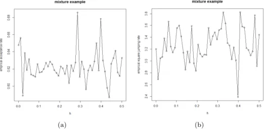
Figure 2.4 Simulation results on the effects ofhon (a) the acceptance rate and (b) the mean jumping distance. The simulation is based on distribution (3) and 20,000 iterations (s21 and s22 are fixed as before). . . 30
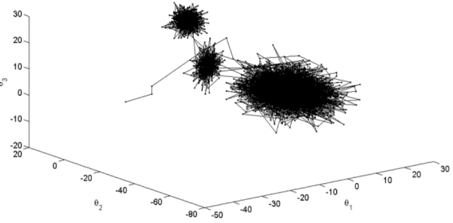
Figure 2.5 Trace of simulated samplings on Θ =R3 for target distribution (2.3.1). The simulation is based on the first 50,000 iterations and thinned by a factor of 10 for easy visualization. Theθ1, θ2 andθ3 denote the
coordi-nates of eachθ. . . 31
Figure 2.6 Comparison of the simulated and theoretical marginal densities for tar-get distribution (2.3.1) based on 150,000 iterations. . . 32
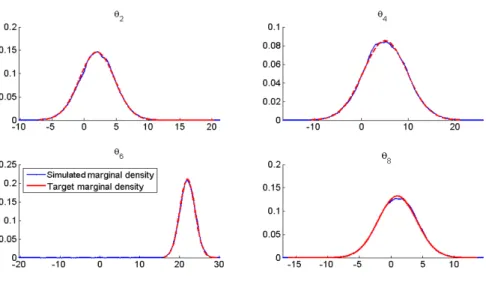
Figure 2.7 Comparison of the simulated and theoretical marginal densities forθ2, θ4, θ6
Figure 2.8 Comparison of the simulated and theoretical marginalcdfs forθ1, θ3, θ5
and θ7 of target distribution (2.3.2) based on 150,000 iterations. . . 33
Figure 2.9 Sample autocorrelations of iterations forλ3,λ6,λ10 and β. . . 36
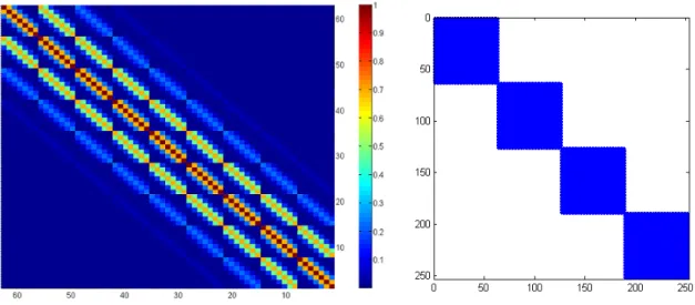
Figure 3.1 Heat map representations of a typical Vq(ηq, γq) (the left panel) and a typical
p
L
q=1
Vq(ηq, γq) (the right panel, where white indicates zero values
of the matrix entries) for ΛL,M withL= 7 andM = 9 andp= 4. . . . 55
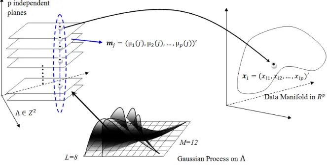
Figure 3.2 A schematic of the BHTC model. The data model is conditional on the prototypes, while the prototype model is the set of Gaussian processes that drive the self-organization. . . 56
Figure 3.3 Demonstration of the rapid decay ofλ0(γq) for L= 7 and M = 9. . . . 59
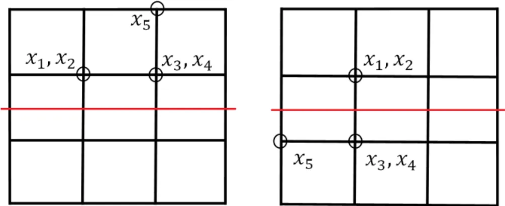
Figure 3.4 Two clusterings are associated with the 3×3 square grid ΛL,M. For a
data set{Xi}5i=1, they are equivalent in “partition risk” (3.4.3).
How-ever, data geometry associated with the frist would typically be more “local” than that of the second. . . 69
Figure 3.5 Two equivalent clusterings with respect to risk (3.4.8) for a data set
{Xi}5i=1. (The black line is the center line of grid.) . . . 71
Figure 3.6 Examples of the HTF surface data and Swiss roll data. Left panel is the HTF surface data, where the shaded area is the semi-sphere. The right panel is the Swiss roll data with two parallel strips that provides two “theoretical” clusters. . . 79
Figure 3.7 Posterior coincidence matrices. Panels (a) and (b) are for the Swiss roll data and wine date, respectively. Panel (a) visualizes that with high posterior probability, the first 40 and the 81th ∼120th data points are within the same group while the remaining data are within another group. Similarly, panel (b) shows three potential clusters with high posterior probability that agrees with the natural clusters. . . 81
Figure 3.8 SOM-visualizations of the optimal BHTC clustering. Panels (a) and (b) are for the Swiss roll data and wine date, respectively. Colored numbers represent the data indices and natural/theoretical clusters. . . 82
Figure 3.9 Demonstrations of{ˆγq∗}pq=1 for measuring “variable importance for the BHTC”. . . 83
Figure 3.10 Comparison of clustering methods based on ψ-statistics and four data sets. The legends for clustering methods are displayed in panel (a). . 86
Figure 3.11 Comparison of clustering methods based on the Rand indices and four data sets. The legends for clustering methods are displayed in panel (a). 87
Figure 3.12 Comparison of clustering methods based on the F5 measures and four
data sets. The legends for clustering methods are displayed in panel (a). 88
Figure 3.13 Triangular array formed by values of Rn(ν) onPn
Λ. . . 101
Figure 4.1 Densities of the feature distributionsF andGin the models for training and predicting sets in Example4.2.1. The dashed line and solid line are respectively optimal decision boundaries for training and predicting. . 116
Figure 4.2 Applying a 3-nearest neighborhood method, we change the decision boundary. The original decision boundary (the solid line) is updated by the new one (the dashed line) for a training set, which is a subset of the original training set and obtained based on distances to feature vectors in the predicting set. The new separation is more effective for classification than the original one. . . 117
Figure 4.3 Illustrative examples for approximatingGby the empirical distribution fromS1q. Using the procedure in part (a) of Step 3 in Algorithm4.2.2, we approximate F by the empirical distribution from S1q with q = 5. The Kolmogorov-Smirnov distance (KS distance) between the S1q-empirical and underlying distributions are reported based on 100 simulations for each value ofn. The KS distance decreases in n. . . 121
Figure 5.1 Lesion size (i.e. the increase of footpad thickness during infection) across time under different type of infections for two type of mice ((A) for C3H, (B) for B6). . . 139
Figure 5.2 Box-Cox plots of the binned measured footpad thickness. (a) and (b) are for the infected and non-infected feet, respectively. . . 139
Figure 5.3 Demonstration of informal diagnostics for MCMC. In (a), mu, sdmouse and lambda1 stand forµ,σm and λ1; and in (b), sdfoot, log theta2 and
pbeta stand forσf, log(θ2) and (−γ). . . 146
Figure 5.4 Fitted responses of the model for two types of mice with three types of infections. The response is the difference between the thickness of the two footpads of a mouse. . . 151
Figure 5.5 Estimated relationship between the unobserved pathogen load and ob-served lesion size across time based on (5.4.2) and discussion on links in Section 5.3.2. For C3H and B6 mice, the cross section dimension of footpad is 40mm2. . . 153
Figure 5.6 Posterior distributions of the effective fitness of pathogens in two types of mice. Panels (a),(b),(c) and (d) are forα1lm−µ1lm,α2lm−µ2lm,α1la−µ1la
ACKNOWLEDGEMENTS
I would like to express my deepest appreciation to my advisors, Professor Stephen Vardeman and Professor Huaiqing Wu for their guidance, patience and support throughout my years at ISU. During my four years of study at the Snedecor Hall, they not only spent tremendous hours proofreading my research papers but also inspired me to conduct research on a very broad range of statistical topics. The philosophy on both academia and life I have learned from them, as well as many invaluable experiences they shared with me, will constantly guide me for my career path and my whole life. I also would like to thank Professor Vardeman for his constant encouragement to me, and he have rebuilt my confidence on life. He embodies the model that I will endeavor to follow in future.
I would also express my gratitude to my committee members. Specially, I want to thank Professor Max Morris for his guidance on the Health Heritage data mining project, and also his constant support and inspiration on my research. I also thank Professor Daniel Nordman and Professor John Jackman for many helpful suggestions and support during my study. I would like to thank Professor Peng Liu for her funding support and helpful discussions on my research work.
From the bottom of my heart, I own my gratitude to my parents, not only for having me in the first place but for believing in me all these years no matter what I have chosen to pursue. I would like to express the love to my wife, who always stays with me with great supports. Finally, thanks go to our precious daughter, Michelle, for the joy she brings to our life and it is her helping me to understand the meaning of life.
CHAPTER 1. INTRODUCTION
1.1 Background
With recently increasing attentions, the statistical machine learning has been considered as a collection of modern statistical methods that employ techniques from machine learning, data mining, optimization, differential geometry and differential equations, etc (Bishop, 2007;
Izenman,2008;Hastie, Tibshirani and Friedman,2009;Ma and Fu,2011;Barber,2012). Two
characteristics distinguish the statistical machine learning from classical statistical methods: the data type and the purpose of data analysis. First, advancements in scientific fields and the computer science over the past few years have made the collection and storage of massive data set less expensive. Data of new types have been generate by a variety of fields: through the microarray or high throughput RNA sequencing experiment (Pierre and Søren,2001); through experiments that frequently collect infectious tissue samples in pathology lab (Zhang, et al.,
2011); through infrastructure such as smart agriculture and power grids; and through websites as deployed in businesses and social networking (Bishop,2007), etc. The new data types have a great impact in statistics that they require and lead to creations of many new statistical methods of inference and prediction. Particularly, the statistical machine learning focuses on those data of new types, such as high-dimensional data with a large number of variables relative to the number of observations, multivariate functional data, or the so called “Big Data” with both large numbers of variables and observations. On the other hand, the statistical machine learning focuses on inference of new types including detecting nonlinear geometric structures in data cloud (manifold learning), identifying intrinsic grouping structures (data clustering), building predictive model for decision making, selecting important variables with or without projections (dimension reductions or variable screenings), and providing data-driven answers
to scientific questions, etc.
With a very broad scope, the statistical machine learning is roughly divided into two sub-fields, the supervised learning and unsupervised learning (mainly clustering and manifold learn-ing) that depends on whether a response being assigned for each observation. Sometimes, a further categorization is mentioned in literature if we considered regression and classification problems separately in the supervised learning regime.
Both the Bayesian method and multivariate statistical methods have been broadly employed in all these three fields in the statistical machine learning. Multivariate statistical methods are extensively applied in the statistical machine learning given the multivariate nature of the data of interest. There are many well-established applications in literature, including the least angle regression (Efron, et al.,2004), nonparametric regression (Izenman,2008), Fisher’s discriminant analysis (Anderson,2003), logistic regression (Hastie, Tibshirani and Friedman,2009), random forest (Breiman,2001), gradient boosting machine (Friedman,2001) etc. We refer toIzenman
(2008) and Hastie, Tibshirani and Friedman(2009) for more examples.
The Bayesian method is adopted to the statistical machine learning in both the concep-tual and technical fashions. For example, the naive Bayes classifier is a widely-used powerful method for classification problems, especially in the high-dimensional settings (Hastie,
Tib-shirani and Friedman, 2009); and it is motivated from the Bayesian concept on optimizing
a posterior risk function. Also, the Bayesian interpretation on the reproducing kernel Hilbert space (RKHS) using Gaussian processes, which provides the foundation of functional data anal-ysis and nonparametric regression, provides another examples of using Bayesian concepts in statistical learning (Rasmussen and Williams,2006). The Bayesian concept also provides an al-ternative shrinkage estimator (that adopt a Dirichlet-Laplace priors as a shrinking prior) in the high-dimensional settings that assembles LASSO’s approach yet provides some optimality for estimation (Bhattacharya, et al.,2014). In addition, as fundamental concepts in the Bayesian framework, model comparison and average play important roles in developing ensemble learning methods such as bagging (Hastie, Tibshirani and Friedman,2009).
Technically, the Bayesian method provides tools to refine existing machine learning method, introduce coherent probabilistic learning models, integrate techniques from other fields
(par-ticularly applied mathematics and statistical mechanics) with machine learning methods, and design new computational methods. For example, the Bayesian variable selection has been widely applied in feature selections in high-dimensional settings (Lee, et al.,2002;O’Hara and
Sillanp¨a¨a, 2009). Combining with the compressive sensing, the Bayesian compressive
regres-sion (Ji, Xue and Carin , 2008; Derin Babacan, Molina and Katsaggelos, 2010; Guhaniyogi
and Dunson, 2013) has also provided an alternative to the screening method (Fan and Lv,
2008), marginal regression (Genovese, et al., 2011) and least angle type regression (that in-cludes LASSO). Neal and Zhang(2006) has presented a so called “Bayesian neural network”, which has been shown powerful for two-classes classification problems (the original problem is given in a classification competition organized by Neural Information Processes Systems (NIPS) in 2003, and the two authors won the competition using the Bayesian neural network). Besides ubiquitous applications in regression and classification problems, the Bayesian method has drawn increasing attentions to data clustering and manifold learning. Deng, Geng, and Liu (2014) has proposed a novel method for clustering character strings based on the Mar-ket BasMar-ket Analysis (MBA) and Bayesian hierarchical models. Their method is efficient to cluster non-alphabetic strings such as Chinese characters. Recently, Yang and Dunson(2013) has introduced a Bayesian manifold “regression” to study nonlinear dimension reduction using Gaussian processes and the nonparametric Bayesian framework. We refer toBarber (2012) for more applications of the Bayesian method in the statistical machine learning.
A challenge for employing the Bayesian method in the statistical machine learning is de-veloping tractable computational schemes. Markov Chain Monte Carlo (MCMC) provides a systematic and efficient treatment to computational issues when we applied the Bayesian method. Both Deng, Geng, and Liu (2014) and Neal and Zhang (2006), for example, used hybrid MCMC to solve the proposed model for inference on the learning problems. To accom-modate news challenges brought by applying the Bayesian method to the statistical machine learning, new MCMC methods are needed. Robert and Casella (2004) provides an extensive reviews on this topic.
Last but not least, multivariate functional data analysis is sometimes also considered falling into the regime of the statistical machine learning. Particularly, it is very important to
iden-tify the principal component directions or effective dimensions for multivariate functional data
(Ramsay and Silverman, 2005; Li and Hsing, 2010). This is closely related to the linear
di-mension reductions (Anderson, 2003; Izenman, 2008). In this dissertation, we will focus on modeling multivariate functional data by differential equations model and drawing reasonable answers to specific scientific questions using the Bayesian approach.
This dissertation would focus on developing an MCMC algorithm for sampling a target distribution, which could be applied to classifications and data clustering that might be mod-eled by mixture models; constructing a Bayesian clustering method to preserve topographic information of data; proposing an classification method based on the weighted bootstrap and ensemble; and reporting the Bayesian analysis of multivariate functional data using differential equations model.
1.2 Literature Review
In this section, a brief literature review would be given for each of the main topic covered from Chapter2 to Chapter 5.
1.2.1 Adaptive MCMC
Markov Chain Monte Carlo (MCMC) is the most used tool for sampling a target probability distribution, and it has a broad application in Bayesian statistical inference and scientific com-putations in statistical physics (Robert and Casella, 2004;Landau and Binder,2005). Tuning parameters are critical for an MCMC algorithm to have good mixing properties. Adaptive MCMC algorithm has been proposed to find satisfactory tuning parameters automatically us-ing the information of a target distribution and/or the previous posterior samples. This elegant solution executes tuning adaptively along the updates of the algorithm. There exists a large literature for this method, see Harrio, Saksman and Tamminen(2001);Andrieu and Moulines
(2005); Atchade and Rosenthal (2005); Atchade (2006) and Roberts and Rosenthal (2009).
Harrio, Saksman and Tamminen(2001) has introduced an adaptive Metropolis algorithm that
uses a repeatedly updated empirical sample covariance matrix from the history of the process as a covariance matrix for the proposal probability function. Atchade (2006) has extended
an adaptive MCMC algorithms, which was based on independence samplers and random-walk Metropolis transition probability kernel, to a more general class of Metropolis-Hastings (MH) algorithms by employing an extra drift term. Similar adaptive schemes were proposed and analyzed byAndrieu and Moulines (2005) and Atchade and Rosenthal(2005).
1.2.2 Data clustering and the self-organizing map
Data clustering focus on learning latent heterogeneity of data vectors and separates them into homogeneous subsets. It has recently played an indispensable role in areas of scientific re-search as diverse as clustering gene transcripts to detect different functional groups on the basis of RNA sequencing data Pierre and Søren (2001) and clustering astronomical data searching new galaxies Izenman (2008). Data clustering has become increasingly important in detect-ing sub-communities in a network, see Arias-Castro, Cand´es and Durand (2011); Jin (2013);
Arias-Castro and Grimmett(2013). Xu and Wunsch (2005) andIzenman (2008) provide more
applications of data clustering. Data clustering also provides tools in learning latent struc-ture in graphical models and assists on estimating high-dimensional covariance matrices, see
Banerjee and Ghosal(2013) for example.
There exists a large number of clustering methods in literature. For example, as one of the most popular clustering methods, the K-means method (Hartigan and Wong, 1979) is a deterministic greedy optimization algorithm and has nonparametric spirit. The agglomerative hierarchical clustering method is also algorithm based method and depends on the concept of distance between clusters that is modeled by the linkage functions (Ward, 1963). Proposed
by Hastie and Stuetzle (1989) and LeBlanc and Tibshirani (1994), the principal curves and
principal surface focus on learning the nonlinear geometry of data cloud, seeMa and Fu(2011) for more discussions on their connections with manifold learning and differential geometries. Motivated from the graph theory, the spectral clustering algorithm performs data clustering based on the spectrum decomposition of the graph Laplacian (Hagen and Kahng,1992). As the weight matrix in formulating the graph Laplacian is defined by the heat kernel, spectral clustering has an intrinsic connection with the Laplace-Beltrami operator and diffusion equa-tions (Belkin and Niyogi,2003). Combining the spectrum clustering and the degree-corrected
block model (DCBM), Jin (2013) has proposed a novel clustering method, the spectral clus-tering on ratios-of-eigenvectors (SCORE), whose optimality of performance is shown under mild deviation assumptions. We refer tovon Luxburg(2007) for more discussions on spectrum clustering. Other clustering methods such as nonnegative matrix factorization, independent component analysis, and dimension scaling, etc. are extensively discussed in literature, see
Hastie, Tibshirani and Friedman(2009) and Izenman (2008).
Different from above clustering methods, the self-organizing map (SOM) was motivated by a dynamical system modeling the neural network and signal propagation. Originally intro-duced byKohonen(1982), it is one of the most used clustering methods for its straightforward expression as an algorithm. The SOM provides a smooth mapping from an input data space to an output prototype space and performs automatically vector quantization (Kohonen,2001;
Yin, 2008). The SOM and its variants have been applied to many regimes including spatial-temporal data modeling (Sang, et al.,2008) and texture segmentations (Ruiz del Solar,1998). SeeEst´evez, Pr´ıncipe and Zegers (2013) andLee and Verleysen(2006) for an extensive review of applications of SOMs. Part of the main objective in this dissertation is to develop a Bayesian clustering method motivated by the SOM.
1.2.3 Dataset shift in classifications
The data quality has a great impact on the classifiers’ performance in classification problems, and it has been discussed extensively in literature including the data complexity (Ho and Basu,
2002), missing values (Hastie, Tibshirani and Friedman,2009;Ghannad-Rezaie, et al.,2010), intrinsic variances (Zhu and Wu,2004), imbalances (Fithian and Hastie,2013) and the dataset shift. Dataset shift has drawn growing attentions as many theoretically well-behaved methods suffers from it in practice. It was in Storkey (2009) dataset shift was first defined formally by “cases where the joint distribution of inputs and outputs differs between training and test stage”. Dataset shift is then categorized into three types. The first type is called the covariate shift, for which the distribution of the input variables changes with respect to the training and test sets. It was first defined by Shimodaira (2000), and has been widely studied in literature (Hand,2006;Yamazaki, et al.,2007;Bickel, Br¨uckner and Scheffer,2009;Gretton et al.,2009).
The second type is referred byStorkey(2009) as the prior probability shift, which is similar to the imbalance problem that the marginal distribution of labels changes between the training and test sets. Cieslak and Chawala (2009) have provided a comprehensive discussion on the dataset shift of the second type. The dataset shift of the third type is usually referred to as the concept shift, in which the conditional distribution of labels on input variables changes between the training and test sets (Widmer and Kubat,1996;Yamazaki, et al.,2007).
Considering the dataset shift, especially the covariate shift, as a consequence of sample se-lection bias or non-stationary environment, many methods have been developed to work under the dataset shift. Some important methods include, for example, the weighted log-likelihood method byShimodaira(2000), the importance-weighted cross-validation bySugiyama,
Kraule-dat and M¨uller(2007), the asymptotic Bayesian generalization error corrections by Yamazaki,
et al.(2007), the discriminative learning by Bickel, Br¨uckner and Scheffer(2009), and the ker-nel mean matching procedure by Gretton et al. (2009). We refer to Qui˜nonero-Candela, et al. (2009) for more discussions on other methods targeting on the prior probability shift and the concept shift. This dissertation would focus primarily on covariate shift, and constructs a weighted bootstrap based classification method to work under the covariate shift.
1.2.4 Statistical inference on differential equation parameters
Differential equations focus on modeling the underlying mechanism of physical (or biological, etc.) systems and have been widely employed. Recently, statistical inference on differential equation parameters has drawn increasing attentions. Many methods have been developed using different statistical approaches. For example, for ordinary differential equations (ODEs),
Jacobsen and Madsen (1996) have proposed a method based on approximation of dynamical
system by multivariate time series, Ramsay et al. (2007) have introduced a nonparametric method using techniques in functional data analysis, and Liang and Wu (2008) and Fan, Wu
and Zhu (2011) have developed another nonparametric approach based on local polynomial
regressions. Cao, Huang and Wu (2011) and Chen and Wu(2008) have discussed methods to accommodate ODEs with time-varying parameters instead of constants. Recently, using the disintegration theorem,Breidt, Butler and Estep(2011) andButler, Estep and Sandelin(2012)
have constructed a measure-theoretic framework to solve inverse problems (basically parameter estimations in statistics) in a more general form.
Given its flexibility and coherence, the Bayesian method have received increasing atten-tions for inference on differential equation parameters. For example, Huang, Liu and Wu
(2006) adopted the Bayesian framework to study an ODE system from virology, Drignei and
Morris (2006) used the Bayesian method to conduct inference on parameters of reaction
dif-fusion equations from the point of view of experimental design (which is an early attempt on parameter estimations of partial differential equations (PDEs)), and a series of methods have been constructed for PDEs from fluid mechanics or differential geometries based on the Bayesian framework and hybrid MCMC in Pavliotis and Stuart (2007); Pokern, Stuart, and
Wiberg(2009);Cotter, Dashti, Robinson and Stuart(2009);Dashti and Stuart(2011) andLee,
McDougall and Stuart (2011). Recently, Knapik, van der Vaart and van Zanten (2013) has
introduced the nonparametric Bayesian method for parameter inference for the heat equation.
1.3 Thesis Organization
This dissertation is organized as follows. The general introduction chapter is followed by four main chapters and ends with a general conclusion in Chapter 6. Each of the four main chapters consists of a journal article. Chapter 2 introduces a new MCMC algorithm based on the geometric information of a target distribution function and the Metropolis-Hastings transition probability kernel. In Chapter 3, we present a Bayesian hierarchial topographic clustering method motivated by the self-organization maps. A MCMC algorithm is reported with details for sampling the posterior distributions of the method parameters, based on which a posterior risk framework is carefully constructed to obtain the approximate optimal clustering. Chapter 4 gives a classification method based on a so called “active set selections” strategy to deal with covariate shift in classification problems. Chapter 5 reports a novel application of using Bayesian methodologies and differential equations model to study the longitudinal data from immunology, and provides sensible answers to some immunobiological challenging questions.
References
Anderson, T.W. (2003). An Introduction to Multivaraite Statistical Analysis. John Wiley &
Sons, Hoboken, NJ.
Atchade, F.Y. (2006). An Adaptive Version For The Metropolis Adjusted Langevin
Algo-rithm With A Truncated Drift.Methodology and Computing in Applied Probability.8235-254.
Arias-Castro, E. and Grimmett, G.R. (2013). Cluster Detection In Networks Using Percolation. Bernoulli.19(2)676-719
Arias-Castro, E., Cand`es, E.J., and Durand, A. (2011). Detection Of An Anomalous Cluster In A Network. The Annals of Statistics.39(1)278-304.
Andrieu, C. and Moulines, E. (2005). On The Ergodicity Properties Of Some Adaptive
Mcmc Algorithms. Annals of Applied Probability.16 1462-1505.
Atchade, F.Y. and Rosenthal, S. J. (2005). On Adaptive Markov Chain Monte Carlo
Algorithms. Bernoulli.5815-828.
Barber, D.(2012).Bayesian Reasoning and Machine Learning. Cambridge University Press.
Banerjee, S. and Ghosal, S. (2013). Bayesian Structure Learning In Graphical.manuscript. Belkin, M. and Niyogi, P. (2003). Laplacian Eigenmaps For Dimensionality Reduction And
Data Representation. Neural Computation.15(6)1373-1396.
Bishop, M.K.(2007).Pattern Recognition and Machine Learning. Springer-Verlag, New York.
Bickel, S., Br¨uckner, M., and Scheffer, T. (2007). Discriminative Learning Under Covariate Shift.Journal of Machine Learning Research.102137-2155.
Breiman, L. (2001). Random Forests. Machine Learning.45(1) 5-32.
Breidt, J., Butler, T., and Estep, D. (2011). A Measure-Theoretic Computational Method For Inverse Sensitivity Problems I: Method And Analysis.SIAM Journal on Numerical Analysis.
Butler, T., Estep, D., and Sandelin, J. (2012). A Computational Measure Theoretic Approach To Inverse Sensitivity Problems Ii: A Posteriori Error Analysis.SIAM Journal on Numerical Analysis.5022-45.
Derin Babacan, S., Molina, R., and Katsaggelos, A.K.(2010). Bayesian Compressive
Sensing Using Laplace Priors. Ieee Transactions On Image Processing.19(1) 53-63.
Bhattacharya, A. Pati, D. Pillai, N.S., and Dunson, D.B. (2014). Dirichlet-Laplace
Priors For Optimal Shrinkage.manuscript.
Cieslak, D.A. and Chawala, N.V. (2009). A Framework for Monitoring Classifiers’ Performance: When and Why Failure Occurs? Knowlegde and Information System.18(1)83-108.
Cao, J., Huang, J.H. and Wu. H.L.(2011). Penalized Nonlinear Least Squares Estimation
Of Time-Varying Parameters In Ordinary Differential Equations. Journal of Computational and Graphical Statistics DOI: 10.1198/jcgs. 2011. 10021
Chen, J.W. and Wu, H.L.(2008). Estimation Of Time-Varying Parameters In Deterministic
Dynamic Models. Statistica Sinica.8 987-1006.
Cotter, S.L., Dashti, M., Robinson, J.C., and Stuart, A.M. (2009). Bayesian Inverse Problems For Functions And Applications To Fluid Mechanics. Inverse Problems 25115008.
Drignei, D. and Morris, M. (2006). Empirical Bayesian Analysis For Computer
Experi-ments Involving Finite Difference Codes. Journal of the American Statistical Association. 101 1527-1536.
Dashti, M. and Stuart, A.M. (2011). Uncertainty Quantification And Weak Approximation Of An Elliptic Inverse Problem. SIAM Journal of Numerical Analysis.492524-2542.
Deng, K, Geng, Z. and Liu, S.J.(2014). Association Pattern Discovery Via Theme
Dictio-nary Models. Journal of the Royal Statistical Society: Series B. 76(2)319-347.
Efron, B., Hastie, T., Johnstone, I., and Tibshirani, R.(2004). Least Angle Regression.
Est´evez, P.A., Pr´ıncipe, J.C., and Zegers, P.(2013).Advances in Self-Organizing Maps.
Springer-Verlag, New York.
Fan, J. and Lv, J. (2008). Sure Independence Screening For Ultrahigh Dimensional Feature
Space. Journal of the Royal Statistical Society: Series B. 70(5)849-911.
Fan, Y., Wu, H.L. and Zhu, L.X. (2011). A Two Stage Estimation Method For Random
Coefficient Differential Equation Models With Application To Longitudinal Hiv Dynamic Data. Statistica Sinica.211145-1170.
Friedman, J.H. (2001). Greedy Function Approximation: A Gradient Boosting Machine. The Annals of Statistics.29(5)1189-1232.
Fithian, W. and Hastie, T. (2013). Local Case-Control Sampling: Efficient Subsampling in Imbalance Data Sets.manuscript.
Genovese, C., Wasserman, L., Jin, J., and Yao, Z.(2011). A Comparison Of The Lasso
And Marginal Regression. Journal of Machine Learning Research.13 2107-2143.
Guhaniyogi, R. and Dunson, D.B. (2013). Bayesian Compressed Regression.manuscript.3
Ghannad-Rezaie, M., Soltanian-Zadeh, H., Ying, H., and Dong, M. (2010). Selection-Fusion Approach For Classification Of Datasets With Missing Values. Pattern Recognition. 43(6)
2340-2350.
Gretton, A., Smola, A., Huang, J. Schmittfull, M., Borgwardt, K., and Sch¨olkopf, B. (2009). Covariate Shift by Kernel Mean Matching, in: Qui˜nonero-Candela, J., Sugiyama, M., Schwaighofer, A., and Lawrence, N.D. (Eds.) Dataset Shift in Machine Learning. The MIT Press.
Hagen, L. and Kahng, A. (1992). New Spectral Methods for Ratio Cut Partitioning and
Clustering. IEEE Transactions on Computer-Aided Design of Integrated Circuits and Sys-tems. 11, 1074-1085.
Hand, D.J. (2006). Rejoinder: Classifier Technology and The Illusion of Progress. Statistical Science.21(1)30-34.
Hastie, T. and Stuetzle, W.(1989). Principal Curves.Journal of the American Statistical
Association. 84, 502-516.
Hastie, T., Tibshirani, R., and Friedman, J.(2009).The Elements of Statistical Learning:
Data Mining, Inference, and Prediction. Springer-Verlag, New York.
Hartigan, J.A. and Wong, M.A. (1979). Algorithm AS 136: A K-means Clustering
Algo-rithm.Journal of the Royal Statistical Society. Series C. 28, 100-108.
Harrio, H., Saksman, E., and Tamminen, J. (2001). An Adaptive Metropolis Algorithm.
Bernoulli.7 223-242.
Ho, T.K. and Basu, M. (2002). Complexity Measures Of Supervised Classification Problems. IEEE Transactions on Pattern Analysis and Machine Intelligence.24(3) 289-300.
Huang, Y., Liu, D. and Wu, H.L. (2006). Hierarchical Bayesian Methods For Estimation
Of Parameters In A Longitudinal Hiv Dynamic System. Biometrics.62413-423.
Izenman, A.I.(2008). Modern Multivariate Statistical Techniques: Regression, Classification,
and Manifold. Springer-Verlag, New York.
Jacobsen, J.L. and Madsen, H.(1996). Grey Box Modelling Of Oxygen Levels In A Small
Stream.Envirometrics.7 109-121.
Ji, S., Xue, Y., and Carin, L. (2008). Bayesian Compressive Sensing. IEEE Transactions
on Signal Processing. 56(6)2346-2356.
Kohonen, T. (1982). Self-Organized Formation of Topologically Correct Feature Maps.
Bio-logical Cybernetics.43, 59-69.
Kohonen, T.(2001). Self-Organizing Maps. Springer-Verlag, New York.
Knapik, B.T., van der Vaart, A.W., and van Zanten, J.H. (2013). Bayesian Recovery Of The Initial Condition For The Heat Equation. manuscript.
Landau, P.D. and Binder K. (2005). A Guide to Monte Carlo Simulations in Statistical
Lee, W., McDougall, D., and Stuart, A.M. (2011). Kalman Filtering And Smoothing For Linear Wave Equations With Model Error.Inverse Problems 27095008.
Li, Y. and Hsing, T. (2010). Deciding The Dimension Of Effecive Dimension Reduction
Space For Functional And High-Dimensional Data. The Annals of Statistics.32(2)407-840.
Liang, H. and Wu. H.L. (2008). Parameter Estimation For Differential Equation Models
Using A Framework Of Measurement Error In Regression Models. Journal of the American Statistical Association. 1031570-1583.
Jin, J. (2013). Fast Community Detection by Score.manuscript.
LeBlanc, M. and Tibshirani, R.(1994). Adaptive Principal Surfaces.Journal of the
Amer-ican Statistical Association. 89, 53-64.
Lee, K.E., Sha, N., Dougherty, E.R., Vannucci, M., and Mallick, B.K.(2002). Gene
Selection: A Bayesian Variable Selection Approach. Bioinformatics.19(1)90-97.
Lee, J.A. and Verleysen, M.(2006).Nonlinear Dimensionality Reduction. Springer-Verlag,
New York.
Manifold Learning Theory and Applications. (2011). Y. Ma and Y. Fu (eds), CRC Press. Neal, R. and Zhang, J. (2006). High Dimensional Classification With Bayesian Nueral Networks
And Dirichlet Diffusion Trees. in I. Guyon, S. Gunn, M. Nikravesh and L. Zadeh (eds), Feature Extraction, Foundations and Applications. Springer, New York, 265-296.
O’Hara, R.B. and Sillanp¨a¨a, M.J. (2009). A Review of Bayesian Variable Selection Methods: What, How and Which. Bayesian Analysis.4(1)85-118.
Pavliotis, G. and Stuart, A.M. (2007). Parameter Estimation For Multiscale Diffusions.Journal of Statistical Physics.127741-781.
Pierre, B. and Søren, B. (2001). Bioinformatics: The Machine Learning Approach. A
Pokern, Y., Stuart, A.M., and Wiberg, P. (2009). Parameter Estimation For Partially Observed Hypo-Elliptic Diffusions.Journal of the Royal Statistical Society Series B.7149-73.
Qui˜nonero-Candela, J., Sugiyama, M., Schwaighofer, A., and Lawrence, N.D. (2009). Dataset Shift in Machine Learning. The MIT Press.
Rasmussen, C.E. and Williams, C.K.I.(2006).Gaussian Processes for Machine Learning.
MIT Press, Cambridge, MA.
Ramsay, J.O. and Silverman, B.W. (2005). Functional Data Analysis. Springer-Verlag,
New York.
Ramsay, J.O., Hooker, G., Campbell, D. and Cao, J.(2007). Parameter Estimation For
Differential Equations: A Generalized Smoothing Approach. Journal of the Royal Statistical Society: Series B. 69741-796.
Robert, P. C. and Casella, G. (2004).Monte Carlo Statistical Methods. Springer-Verlag,
New York.
Roberts, O. G. and Rosenthal, S. J. (2009). Examples of adaptive MCMC. Journal of
Computational and Graphical Statistics. 18349-367.
Ruiz del Solar, J. (1998). TEXSOM: Texture Segmentation using Self-Organizing Maps.
Neurocomputing. 21, 7-18.
Sang, H., Gelfand, A.E., Lennard, C., Hegerl, G., and Hewitson, B. (2008).
Inter-preting Self-Organizing Maps Through Space-Time Data Models. Annals of Applied Statis-tics. 2, 1194-1216.
Shimodaira, H. (2000) Improving Predictive Inference Under Covariate Shift by Weighting the Log-Likelihood Function. Journal of Statistical Planning and Inference.90(2) 227-244.
Storkey, A. (2009). When Training and Test Sets Are Different: Characterizing Learning Trans-fer. in: Qui˜nonero-Candela, J., Sugiyama, M., Schwaighofer, A., and Lawrence, N.D. (Eds.) Dataset Shift in Machine Learning. The MIT Press.
Sugiyama, M., Krauledat, M., and M¨uller, K.R. (2007). Covariate Shift Adaptation By Impor-tance Weighted Cross Validation. Journal of Machine Learning Research.8 985-1005.
von Luxburg, U. (2007). A Tutorial On Spectral Clustering. Statistics and Computing.17,
395-416.
Ward, J.H. (1963). Hierarchical Grouping To Optimize An Objective Function. Journal of
the American Statistical Association.58, 236-244.
Widmer, G. and Kubat, M. (1996). Learning in the Presence of Concept Drift and Hidden Contexts. Machine Learning.2369-101.
Xu, R. and Wunsch, D. (2005). Survey Of Clustering Algorithms. IEEE Transactions on
Neural Networks. 16, 645-678.
Yang, Y. and Dunson, D.B.(2013). Bayesian Manifold Regression. manuscript.
Yamazaki, K., Kawanabe, M. Watanabe, S., Sugiyama, M., and M¨uller, K.R. (2007). Asymp-totic Bayesian Generalization Error When Training and Test Distributions Are Different. Proceedings of the 24th International Conference on Machine Learning, ICML 07. ACM. New York, NY. 1079-1086.
Yin, H. (2008). Learning Nonlinear Principal Manifolds by Self-Organising Maps. Principal
manifolds for data visualization and dimension reduction, Lecture Notes in Computational Science and Engineer.58, 68-95.
Zhang, G.L., Lin, H.H., Keskin, D.B., Reinherz, E.L., and Brusic, V. (2011).
Dana-Farber Repository For Machine Learning In Immunology.Journal of Immunological Methods.
374(1-2) 18-25.
Zhu, X. and Wu, X. (2004). Class Noise v.s. Attribute Noise: A quantitative Study.Artificial Intelligence Review.22(3)177-210.
CHAPTER 2. A GEOMETRICALLY ADAPTIVE
METROPOLIS-HASTINGS ALGORITHM WITH GAUSSIAN CALIBRATION
A paper under revision for the Bayesian Analysis
Wen Zhou, Stephen B. Vardeman, and Huaiqing Wu
Abstract
The local curvature characterizes a smooth function’s shape. For the purpose of sampling a target distribution, the local curvature of the corresponding probability density function is par-ticularly informative. We propose an adaptive Markov Chain Monte Carlo (MCMC) algorithm based on the Metropolis-Hastings (MH) probability transition kernel and the local curvature of a target density. A bounded Gaussian calibration strategy for the proposed algorithm is moti-vated by the relationship between the acceptance rate and the tuning parameter of the proposal distribution in an MH algorithm for sampling a standard normal distribution. The proposed algorithm balances the expected acceptance rate against the mobility of the algorithm across the state space. Simulation studies demonstrate that the proposed algorithm provides good performance when sampling densities with highly variable local curvatures (such as mixture distributions). Theoretical convergence results are presented for the proposed algorithm.
Keywords: Adaptive Markov Chain Monte Carlo, Bayesian statistics, bounded Gaussian calibration, curvature, finite difference, Metropolis-Hastings algorithm, simulation, statistical computation
2.1 Introduction
Markov Chain Monte Carlo (MCMC) is widely used and studied as a powerful tool for sampling a target probability distribution. It is of particular interest for Bayesian statistical inference and scientific analysis in statistical physics [Robert and Casella (2004);Landau and
Binder (2005)]. An MCMC algorithm is typically chosen from among those whose transition
probability functions (transition kernels) have an invariant (stationary) probability measure being the target distribution. The choice of the particular transition probability function is up to the user and determines the performance of the MCMC algorithm. The transition probability function typically has tuning parameters, and finding appropriate values of the parameters is critical to satisfactory algorithm performance but is often difficult in practice.
Motivated by attempts to automatically find satisfactory tuning parameters, adaptive MCMC has been proposed. This is an elegant solution to the problem of parameter selection where tuning is executed adaptively along the progress of updates of the algorithm [Harrio, Saksman
and Tamminen (2001);Andrieu and Moulines (2005);Atchade and Rosenthal (2005);Atchade
(2006);Roberts and Rosenthal (2009)].
Harrio, Saksman and Tamminen (2001) proposed an adaptive Metropolis algorithm that
uses a repeatedly updated empirical sample covariance matrix from the history of the process as a covariance matrix for the proposal probability function. Atchade (2006) extended adaptive MCMC from algorithms based on independence samplers and from random-walk Metropolis algorithms to a more general class of Metropolis-Hastings (MH) algorithms by employing an extra drift term, which is modeled by the gradient of the target log density. The proposed adaptive scheme in Atchade (2006) is a stochastic-approximation algorithm that adjusts the covariance matrix recursively. Similar adaptive schemes were proposed and analyzed by
An-drieu and Moulines (2005) and Atchade and Rosenthal (2005).
This work is motivated by a perspective different both from estimating an overall covariance matrix for MH proposal densities and from adapting to the gradient of the target density. In the numerical optimization community, it is natural to use information concerning local curvatures of objective functions to improve convergence rates. (For example, the quasi-Newton methods
can provide a second-order convergence rate in contrast to the steepest descent method’s first-order rate [Nocedal and Wright (1999)].) Here, we use an approximate local curvature (encoded in a finite-difference quotient) of a target log density in an adaptive MCMC algorithm. The curvature reflects the local geometry of the target density, and we use that information to set the proposal distribution’s variance structure. The variance of a proposal distribution affects the expected acceptance rate of proposals, which is important for obtaining satisfactory performance of the adaptive MCMC. Motivated by the performance of a (fixed normal) MH algorithm in sampling a target normal distribution, we propose a bounded calibration strategy in hopes of guaranteeing a satisfactory overall acceptance rate for the adaptive MCMC. By adapting to local geometry and using the proposed strategy, the algorithm provides both a high acceptance rate and satisfactory mobility across the state space. The scheme uses only information derived from the state at stepn−1 for setting the transition mechanism to state
n, and therefore possesses the same Markov property as does the classical MH algorithm. So it is easy to implement the proposed algorithm in practice and relatively easy to establish its theoretical convergence results.
The rest of the article is organized as follows. Section 2.2provides the motivation for and formulation of the geometrically adaptive MH algorithm. Section2.3presents some simulation studies demonstrating the performance of the proposed algorithm. Some convergence results are stated in Section 2.4. Discussion and conclusions are given in Section2.5.
2.2 The New Adaptive Metropolis-Hastings Algorithm
We motivate and present the new MH algorithm for Θ⊂Rin Sections 2.2.1and2.2.2. An extension of the algorithm to Θ⊂Rp withp >1 is given in Section2.2.3.
2.2.1 Motivation for the algorithm
In the original MH algorithm, a new sampling from the target distributionF(θ) is generated based on a proposal distribution whose density isJ(·|θc, σ2) with some tuning parameter(s) that
we here denote as σ2, whereθc stands for the current state of the sampling process. Assume
has a densityf(θ). A proposal, denoted byθ∗, is accepted with probability p= min f(θ∗)J(θc|θ∗, σ2) f(θc)J(θ∗|θc, σ2) ,1 .
As in the standard acceptance-rejection algorithm [Robert and Casella (2004)], iff(·)/J(·|θc, σ2) is absolutely continuous on Θ, the acceptance rate for the MH algorithm at θc is
ρ= E min f(θ∗)J(θc|θ∗, σ2) f(θc)J(θ∗|θc, σ2),1 = 2P f(θ∗)J(θc|θ∗, σ2) f(θc)J(θ∗|θc, σ2) ≥1 . (2.2.1)
The acceptance rate measures the performance of the algorithm in some sense. Hereσ2 controls the expected deviation of a new sampling, θ∗, away from the part of Θ with high probability mass conditional onθc.
We focus on the normal MH algorithm by lettingJ(·|θc, σ2) be the N(θc, σ2) density so that
σ2 is the proposal variance. If we sample an N(0, σt2) distribution using a normal MH sampler with the proposal densityJ(·|θc, σ2p), the expected acceptance rate is then
ρ= 1 σtσpπ Z R2 I(y2< x2)e− x2 2σ2t− (y−x)2 2σ2p dydx = 1 π σp σt −1Z R2 h I(y2 < x2)e−x 2 2 i e− (y−x)2 2 σp σt −2 dydx (2.2.2) = √1 2π Z R e−x 2 2 " 2Φ 2|x| · σp σt −1! −1 # dx,
where Φ(·) is the cumulative distribution function (cdf) of N(0,1). We will denote this expected acceptance rate byρ σp σt .
Note thatρis decreasing inσp/σtin (2.2.2), lim σp/σt→∞
ρ= 0,and lim
σp/σt→0
ρ= 1. From Figure
2.1, for example, the expected acceptance rate is about 60% if σp = σt and it drops to 20%
if σp = 6σt. For sampling normal distributions using a normal MH algorithm, we therefore can controlρ by adjusting the ratioσp/σt. Smallσp/σt increases the chance of a new proposal
being accepted but sacrifices mobility around the state space, while largeσp/σtmay provide a process that takes large steps but leads to low acceptance rate. One might simply match the proposal variance to the variance of the target distribution, i.e., take σp2≈σ2t; or alternatively, one might choose σp2 ≈c2optσ2t wherecopt = 2.4 is an “optimal” constant suggested byGelman et al. (2004). (copt= 2.4/
√
Figure 2.1ρ(σp/σt) in (2.2.2).
Notice that if φ(θ;µ, σt2) is the N(µ, σt2) density then
− d2 dθ2 logφ(θ;µ, σ 2 t) −1 =σ2t. (2.2.3) In general, a smooth density functionf(θ) might be approximated locally by a normal density with the same curvature, and (2.2.3) suggests how that might be related to a kind of “local curvature” of the target density. We are therefore motivated to consider using information about the local curvature of logf(θ) at the current state as an adaptive surrogate for the variance of the target distribution, i.e., we consider
˜ σ2 := ˜σ2(θc) = −d 2 dθ2logf(θ) −1 θ=θc
for use in an MCMC algorithm. We calibrate the proposal variance of a normal MH sampler to an adaptively generated ˜σ2, i.e., use roughly σp2 = ˜σ2 or σ2p =c2optσ˜2 and thereby guarantee good performance of the algorithm where the target is normal. The expectation is that the good performance carries over to more complicated cases on nonconstant curvature of a target log density.
Geometrically, f(θ) is locally flat if the curvature of f(θ) on a log scale is small at the current state. The adaptive proposal variance is then large and grants the new proposal large mobility to move to distant regions in Θ. Hence, the Gaussian calibration can be expected to adaptively balance local acceptance rate and mobility around the state space.
2.2.2 A geometrically adaptive Metropolis-Hastings algorithm for Θ⊂R
We use the local curvature of the target log density to provide local geometric information concerning the target distribution F(θ). The local curvature is quantified by the second-order derivative of the log density function. A number of approaches could provide approximate derivatives, such as finite-difference scheme, automatic differentiation, and symbolic differen-tiation. We use a finite-difference method because it is straightforward and provides control on approximation errors. The local curvature of g(θ) at θ0 is quantified by the second-order
derivative of g atθ0. Ifg(θ)∈C3(Θ), then
g00(θ)≈ Hh(g) := g(θ)−2g(θ−h) +g(θ−2h)
h2 , (2.2.4)
where the approximation error is O(h) by Taylor’s theorem. Equation (2.2.4) provides the backward difference quotient forg(θ).
We assume that the target distribution F(θ) is absolutely continuous with respect to the Lebesgue measure on Θ with densityf(θ) such that f(θ)∈C3(Θ),f(θ)>0, and d2logdθ2f(θ) <0
on Θ, so that the logarithm of f(θ) is third-order continuously differentiable with respect to
θ. The local curvature of the log density of F(θ) is approximated by Hh(log(f)), and ˜σ2 is approximated by−H−h1(log(f)).
Numerical approximation of ˜σ2 could perform badly in two situations potentially
encoun-tered in an MCMC simulation. First, the approximate curvatures might not be robust on the boundary of a bounded Θ. Second, a target density could be essentially zero and “nearly” flat over most of Θ, and without some modification the algorithm could produce widely varying proposals that could tend to “jump past” a small region of large density. We propose to resolve these issues by bounding the adaptively generated tuning parameter ˜σ2 with some pre-chosen constantss21 ands22, i.e., by setting
σ2p := min max −H−h1(log(f)) θ=θc, s 2 1 , s22 , (2.2.5)
or σ2p :=c2opt·min max −H−1
h (log(f))|θ=θc, s
2 1
, s22
. In practice, s21 and s22 can be chosen so that usually they do not affect ˜σ2, yet they guard against the pathologies that could follow from directly setting σ2p equal to −H−h1(log(f))
θ=θc or −c 2 optH −1 h (log(f)) θ=θc. We call (2.2.5) the
bounded Gaussian calibration, as it is motivated by the relationship between the acceptance rate of MH sampling of a target normal distribution and the fixed variance of the normal proposal distribution.
For Θ ⊂ R, we thus have an MH algorithm adapting to geometric properties of target distributions as below.
Algorithm 2.2.1. (Geometrically adaptive Metropolis-Hastings algorithm on R)
Step 1. Initialize the algorithm by randomly choosing θ0 ∈ Θ, choose a small value of h > 0,
select s21 < s22, and letj = 1. Step 2. Calculate ˜ σ2j−1 =− 1 Hh(log(f)) θ=θj−1 . (2.2.6)
Step 3. Sample a new proposal
θ∗ ∼N θ|θj−1, c2·min(max(˜σ2j−1, s21), s22)
,
where N denotes the family of normal distributions (normal for Θ = R, and truncated normal for Θ R) with meanθj−1 and variancec2·min(max(˜σ2j−1, s21), s22),wherec2= 1
orc2 =c2opt.
Step 4. Acceptθ∗ in Metropolis-Hastings fashion. That is, take
θj =W θ∗+ (1−W)θj−1,
whereW ∼Bernoulli(r) for
r = min 1, f(θ ∗)·J(θ j−1|θ∗, c2·min(max(˜σ∗2, s21), s22)) f(θj−1)·J(θ∗|θj−1, c2·min(max(˜σj2−1, s21), s22)) ! ,
where ˜σ2∗ is defined by (2.2.6) with θ=θ∗,J is the density of the proposal distribution, and c2= 1 or c2 =c2opt.
2.2.3 Extension of the algorithm to Θ⊂Rp with p >1
We extend Algorithm2.2.1toRp by using the inverse of an approximate Hessian matrix of the log density to set the covariance matrix of the proposal distribution.
2.2.3.1 Approximating the local curvature by a finite-difference scheme
We employ a finite-difference scheme to approximate the local curvature of a function g(θ) at θ0 ∈ Rp, which is itself quantified by the Hessian of g at θ0. If g(θ) ∈ C3(Θ), Taylor’s
theorem implies
∇2g(θ)q≈ ∇g(θ)− ∇g(θ−q) (2.2.7)
and
∇g(θ) =∇g(θ−q) +∇2g(θ−q)q+O(||q||2)
forq∈Rp. By letting q=hei whereei is the unit vector in the ith direction, (2.2.7) implies
∇2g(θ)ei ≈
∇g(θ)− ∇g(θ−hei)
h , (2.2.8)
where the error of approximation is O(h). We therefore have the approximate Hessian of g(θ) defined by
[Hh(g)]ij :=
g(θ)−g(θ−hei)−g(θ−hej) +g(θ−hei−hej)
h2 (2.2.9)
whose approximation error is||Hh(g)− ∇2g||F =O(h
√
p), where||M||F =
p
tr(M0M) denotes the Frobenius norm of ap×pmatrixM. By choosingh=o√1
p
, the error can be controlled to be of order o(1).
Assume the density function f(θ) ∈ C3(Θ) is positive, and that ∇2log(f)(θ) is negative
definite on an open Θ ⊂ Rp. Then H
h(log(f)) provides a candidate approximation for a
local covariance matrix Σ of a multivariate normal component of a target distribution in that
−H−1
h (log(f))≈Σ.
Note thatHh(log(f)) is automatically symmetric and has a spectral decomposition
for a diagonal Λh = diag(λ1, λ2,· · · , λp). We adjustHh(log(f)) by defining for some small >0,
˜
λi = sgn(λi) max(,|λi|) and take ˜Λh = diag
˜
λ1,· · ·,λ˜p
.Then for pre-selected s2
1 < s22, we
apply the bounded Gaussian calibration (2.2.5) to produce for eachi= 1,2,· · ·, p, ˜ ˜ λi:= min max(−˜λ−i 1, s21), s22. (2.2.10) Let ˜ ˜ Λh:= diag ˜ ˜ λ1,· · · ,λ˜˜p (2.2.11) and define ∆h2f(θ) :=QhΛ˜˜hQ0h. (2.2.12)
Then ∆2hf(θ) is symmetric and positive definite, and thus provides a legitimate covariance matrix for a Gaussian proposal distribution making use of local geometric information about the target density.
Remark 2.2.2. Direct application of bounded Gaussian calibration to the diagonal compo-nents of −QhΛ˜hQh
−1
may not result in a valid covariance structure. Expressions (2.2.10 )-(2.2.12) are like (2.2.5) and guarantee a legitimate covariance structure for the proposal distri-bution.
2.2.3.2 Extension of the algorithm for general p
The geometrically adaptive MH algorithm for a multivariate distribution is defined by using the finite-difference quotient of log(f), quantity (2.2.9) with g = log(f), and the calibrated version is defined by (2.2.10)-(2.2.12).
Algorithm 2.2.3. (Geometrically adaptive Metropolis-Hastings algorithm onRp withp >1)
Step 1. Initialize the algorithm by randomly choosingθ0 ∈Θ⊂Rp, choose a small h >0, select
s21< s22, and let j= 1.
Step 2. Calculate ∆2h,j−1(f) := ∆2hf(θj−1) as in display (2.2.12) withθ=θj−1.
Step 3. Sample a new proposal
θ∗∼N θ|θj−1, c2∆2h,j−1(f)
where N denotes the family of multivariate normal distributions (multivariate normal for Θ =Rp, and truncated multivariate normal for Θ Rp) with meanθj−1 and covariance
c2∆2h,j−1(f) withc2 = 1 orc2 =c2opt, wherec2opt = 2.42/p as suggested byGelman et al.
(2004).
Step 4. Acceptθ∗ in Metropolis-Hastings fashion. That is, take
θj =Wθ∗+ (1−W)θj−1,
whereW ∼Bernoulli(r) and
r = min 1, f(θ∗)·J θj−1|θ∗, c2∆2h,∗(f) f(θj−1)·J θ∗|θj−1, c2∆2h,j−1(f) ,
where ∆2h,∗(f) is defined by (2.2.12) withθ=θ∗,J is the density of the proposal distri-bution, andc2 = 1 or c2=c2opt.
Step 5. Repeat Step 2 to Step 4 forj= 1,2,· · ·.
Remark 2.2.4.
1. For high-dimensional target distributions, computation of ∆2h(f) involves a spectral de-composition whose computational complexity is O(p3) and introduces heavy computa-tional burdens. In practice, an alternative is to use only the diagonal components (and a proposal distribution with a diagonal covariance matrix) instead of the full matrix to reduce computation complexity.
2. The performance of the algorithm may depend on the choice of (s1, s2). In practice,
one can select (s1, s2) based on simulation results from short preliminary runs of the
algorithm.
2.3 Numerical Studies
2.3.1 Simulation studies for Θ⊂R
Denote by N(µ, σ2) the normal distribution with mean µ and variance σ2, Gamma(α, β) the Gamma distribution with shape and scale parametersα andβ, anddF/dλthe probability density function for F with respect to the Lebesgue measureλon Θ.
We demonstrate the performance of Algorithm2.2.1for Θ⊂Rwith four target distributions forθ:
1. θ∼Gamma(α, β) withα= 2 and β= 0.5, 2. θ∼F where
dF
dλ(θ)∝(1 + sin
2(3θ))·(1 + cos4(5θ))·e−θ2/2,
3. θ ∼ F where F is a classical normal mixture distribution, F =
3 P i=1 ρiN(µi, σi2) with µ= (−20,5,20)0,σ2= (9,100,16)0, and ρ= (0.45,0.1,0.45)0, and 4. θ ∼F where F = 3 P i=1
ρiFi, F1 = Gamma(2,0.3), F2 = N(−30,100) and F3 = N(30,16)
withρ= (0.45,0.1,0.45)0.
Distribution (2) is a standard example for slice sampling methods as discussed in Robert and
Casella (2004); distributions (3) and (4) are used widely to model latent variables,
classifica-tions, and discriminant analysis [Bishop (2007);Hoff (2009)].
Figures 2.2 and 2.3 provide comparisons between approximate and target densities and comparisons between approximate and target cdfs for the target distributions. All the simu-lations were run for 55,000 iterations starting from a randomly chosenθ0, and 50,000 samples
were retained after the first 5,000 burn-in iterations. We set the difference-quotient parameter
h = 0.01 for the simulations and the scale parameter c2 = 1. The bounding parameters were
s2
1 = 10−4, s22 = 104 for target distributions (1),(3) and (4), and s21 = 0.8, s22 = 104 for target
distribution (2). The truncated normal distribution was used as the proposal distribution in Algorithm2.2.1for target distribution (1), and the normal distribution was used for the other target distributions.
The agreements between simulated and target densities and cdfs in Figures 2.2 and 2.3
(a) (b)
(c) (d)
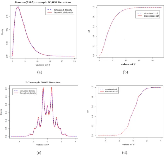
Figure 2.2 Simulation results for distributions (1) and (2) using Algorithm2.2.1based on 50,000 iterations. Panels (a) and (c) are the comparisons between simulated and target den-sities for distributions (1) and (2); panels (b) and (d) are the comparisons between the simulated and target cdfs for distributions (1) and (2).
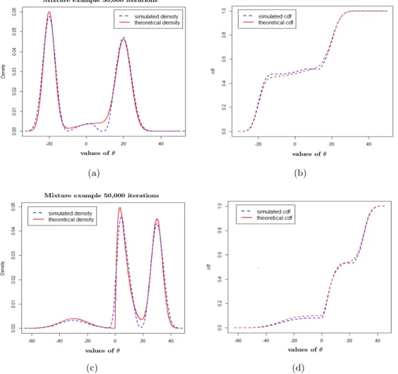
demonstrates that the algorithm performs well to reproduce target distributions with multiple and widely separated modes. The proposed algorithm can capture all the modes and the distributions simultaneously as shown in Figure 2.3, though there is a slight mismatch for the densities, which can be attributed to the relatively small number of iterations.
To compare the performances of the proposed algorithm and standard MH algorithms, we also sampled target distributions (1)-(4) using standard MH algorithms with normal proposal distributions with fixed variances σ2
p = 1 (denoted by MH1), σp2 = 100 (denoted by MH100),
(a) (b)
(c) (d)
Figure 2.3 Simulation results for distributions (3) and (4) using Algorithm2.2.1based on 50,000 iterations. Panels (a) and (c) are the comparisons between simulated and target den-sities for distributions (3) and (4); panels (b) and (d) are the comparisons between the simulated and target cdfs for distributions (3) and (4).
We also sampled the target distributions using our proposed algorithm with scale parameter
c2 =c2opt for further comparisons (this will be denoted as Algorithm2.2.1opt).
The initial states were the same as those used with the proposed adaptive algorithm. Ta-ble 2.1 reports the absolute difference between the simulated and target means (|µ−µˆ|), the Kolmogorov-Smirnov (KS) distance between the simulated and target cdfs, the empirical ac-ceptance rate (AcR), and the root mean square jump (AvJ) defined byd:=pE||θn−θn−1||2.
In terms of representing the target distribution’s mean and reconstructing the target distri-bution (measured by a small KS distance), the proposed algorithm (with c2 = 1 or c2 =c2opt)
Table 2.1 Comparisons between Algorithm 2.2.1 with c2 = 1 andc2 =c2opt and standard MH algorithms with normal proposal distributions with different fixed variances based on 50,000 iterations.
Algorithm |µ−µˆ| KS distance AcR AvJ
distribution (1) Algorithm2.2.1 0.0041 0.0074 0.5886 1.5797 MH1 0.0315 0.0090 0.8982 0.8680 MH100 0.0170 0.0063 0.3954 2.1438 MHopt 0.0237 0.0076 0.4101 1.6054 Algorithm2.2.1opt 0.0243 0.0084 0.4938 2.1538 distribution (2) Algorithm2.2.1 0.0004 0.0040 0.6478 0.6042 MH1 0.0207 0.0100 0.6403 0.6405 MH100 0.0110 0.0210 0.1148 0.5490 MHopt 0.0043 0.0036 0.4601 0.8138 Algorithm2.2.1opt 0.0022 0.0042 0.4685 0.8309 distribution (3) Algorithm2.2.1 0.3181 0.0292 0.6730 2.5827 MH1 9.1807 0.3732 0.9235 1.6952 MH100 1.2051 0.4420 0.4495 4.3957 MHopt 0.2310 0.0382 0.4251 3.9277 Algorithm2.2.1opt 0.7238 0.0336 0.4220 4.0473 distribution (4) Algorithm2.2.1 0.0399 0.0347 0.6006 3.1403 MH1 4.5426 0.9005 0.9214 1.7066 MH100 10.8373 0.3986 0.8848 10.1882 MHopt 0.1154 0.0215 0.3970 6.2287 Algorithm2.2.1opt 0.0496 0.0423 0.3968 6.3644
performs as well as the standard MH algorithms with fixed variances for target distribution (1), and outperforms the algorithms MH1 and MH100 for target distributions (2)-(4). For
re-producing the target distributions, the proposed algorithm (withc2 = 1 orc2 =c2opt) performs very similarly to MHopt, the standard MH algorithm with the optimal scale parameter and the
true target variance. Regarding the acceptance rate and jumping ability, Algorithm 2.2.1opt
behaves like MHopt; the proposed algorithm withc2 = 1 balances the acceptance rate and root
mean square jump size in a slightly different way.
In general, the proposed algorithm did a better job than MH1 and MH100 at balancing the
acceptance rate and jumping distance, particularly for sampling the mixture distributions like target distributions (3) and (4). For the mixture distributions with widely separated modes