Computer Science and Artificial Intelligence Laboratory
Technical Report
MIT-CSAIL-TR-2015-032
November 24, 2015
Representation Discovery for
Kernel-Based Reinforcement Learning
Dawit H. Zewdie and George Konidaris
Representation Discovery for Kernel-Based
Reinforcement Learning
Dawit H. Zewdie
Learning and Intelligent Systems Group MIT, CSAIL
Cambridge, MA 02139
George Konidaris
Intelligent Robot Lab Duke University Durham, NC 27708
Abstract
Recent years have seen increased interest in non-parametric reinforcement learn-ing. There are now practical kernel-based algorithms for approximating value functions; however, kernel regression requires that the underlying function being approximated be smooth on its domain. Few problems of interest satisfy this
re-quirement in their natural representation. In this paper we definevalue-consistent
pseudometric (VCPM), the distance function corresponding to a transformation
of the domain into a space where the target function is maximally smooth and thus
well-approximated by kernel regression. We then presentDKBRL, an iterative
batch RL algorithm interleaving steps of Kernel-Based Reinforcement Learning and distance metric adjustment. We evaluate its performance on Acrobot and Pin-Ball, continuous-space reinforcement learning domains with discontinuous value functions.
1 Introduction
Kernel-based reinforcement learning (KBRL) methods have recently begun to receive significant research attention [1, 2, 3, 4, 5]. These algorithms have the virtue of being non-parametric: their computational complexity scales with the amount of data, rather than with the size of the state
space; consequently, they are a promising means of avoiding the so-calledcurse of dimensionality,
where the number of parameters in a parametric representation of a general value function scales exponentially with the dimensionality of the state space.
Key to these algorithms is the use of kernel regression to extrapolate values. Kernel regression is a smooth-function approximation technique that performs all computation in terms of distance in the state space.
Kernel regression has difficulty modelling discontinuous functions. This difficulty can be alleviated by adding more data, but doing so is often undesirable. We show that changing the distance metric used in the regression can efficiently resolve the difficulties. Existing metric learning algorithms are
not, in general, capable of dealing with discontinuities. We introduce the notion of avalue-consistent
pseudometric(VCP) and show that it allows kernel-regression to model discontinuous functions. We then present a novel iterative algorithm for approximating the VCP, and evaluate its performance on Acrobot and PinBall, two reinforcement learning domains with discontinuous value functions.
2 Background
Reinforcement learning [6] problems are typically formalized as Markov Decision Processes
of states,Ais a finite set of actions,T :S×A×S→[0,1]is an expression of the probability that
a given action will result in a particular state transitionR:S×A×S→Ris an expression of the
reward received for each possible state transition, andγis a discount factor specifying how much
the agent prefers immediate rewards to future ones. The agent starts the process in some start state,
s0, and chooses an actionatbased onstat every time stept, causing the state to change to statest+1
with probabilityT(st, at, st+1), and the agent to receive rewardrt =R(st, at, st+1). The reward
and transition functions are assumed to be unknown; the agent must learn how to act by observing sample rewards and transitions. In this paper, we assume that the agent is given a batch of sample transitions from which to learn.
The agent picks actions by a policyπ : S → A. The total reward the agent can expect when
followingπstarting from statesis denotedVπ(s) =EP
iγiri|s0=s, ai=π(si). The agent’s
objective is to maximize thisreturn, by finding a policy,π∗, such thatVπ∗
(s) = maxπVπ(s)for all
statess. It is convenient to think in terms of the value of a state-action pair,Qπ(s, a), the expected
return when taking action,a, in state,s, then followingπforever after.Vπ(s) = maxaQπ(s, a)
When the set of states is small and finite, an MDP can be efficiently solved by value iteration, which
uses dynamic programming to findV andQsatisfying
Q(s, a) = X
s0∈S
T(s, a, s0) [R(s, a, s0) +γV(s0)].
Solving MDPs with continuous state spaces is less straightforward. Popular techniques include LSTD [8], and Sarsa [9] which try to approximate the value function parametrically. With the right parametric form, these algorithms can produce high quality solutions from very little data; however, no amount of data can help them produce a good solutions when they assume the wrong form. By contrast, non-parametric methods represent the value function directly in terms of the data. This avoids the need for assumptions about value function form and allows the complexity of the fit generated to scale naturally with the amount of data. We are interested in improving KBRL, one particular non-parametric algorithm.
2.1 Kernel-Based Reinforcement Learning
KBRL [1] is a non-parametric value function approximation algorithm for continuous MDPs. It is a three-step process that solves the MDP using a set of sample transitions. The first step constructs a finite approximation of the MDP from the samples, the second step solves that finite approximation, and the third step interpolates that solution to the original state space.
KBRL takes as input a set of sample transitions, Sa = {wa
i = (sai, rai,sˆai) | i = 1, . . . , na},
resulting from each action, a. From these transitions, KBRL constructs a finite MDP, M0 =
hS0, A, T0, R0, γi). The new state space,S0, is the set of sample transitions, so|S0|=n=P ana.
The new reward function isR0(wa
i, a0, wa 0 j ) =ra
0
j . The new transition functionT0is defined as
T0(wa i, a0, wa 00 j ) = 0 ifa0 6=a00 κa0(ˆsai, saj00) otherwise,
whereκa(·,·)is some similarity function constrained to be nonnegative, decreasing in the distance
between its two arguments, and satisfyingPiκa(s, sa
i) = 1for all s ∈ S. It is convenient to
think ofκas being the normalized version of some underlyingmother kernel,k, so thatκa(s, sai) =
k(b−1d(s,sa i))
P
jk(b−1d(s,saj)) wheredis a metric andbis a bandwidth. There is a bias-variance trade-off to be
made when choosingb; bias decreases withbwhile variance increases [1]. Except where stated
otherwise, we use a Gaussian as our mother kernel throughout this paper.
There is work [2] exploring the possibilities for similarity functions (trees, nearest neighbours, and
grid-based approximations), but all of it uses Euclidean distance,dEuc, as the metric. The
justifi-cation is that the value function is assumed smooth—that nearby points have similar values. When
it usesdEuc, KBRL can be seen as using local averaging to approximate the transition, reward, and
Q-value functions. In the next section we show what happens when the smoothness assumption is not met.
KBRL solves forV0, the value function ofM0 using some finite MDP solver then generalizes it to
Musing the equation
Q(s, a) = X
wa i∈Sa
κa(s, sa
i) [ria+γV0(wai)].
Note that the size of the finite model, M0 constructed by KBRL is equal to the number of
sam-ple transitions. This makes solving it computationally intensive, even when using a sparse kernel;
however, an approximate solution toM0can be found efficiently if its transition probability matrix
is replaced by a low-rank approximation [5]. Kernel-based stochastic factorization (KBSF) takes advantage of this property, using a stochastic factorization of the matrix as the low-rank approxima-tion. KBSF takes time linear in the amount of data and a constant amount of space that depends only on the desired approximation coarseness. Though we only provide proofs and results for KBRL, the ideas presented in this paper can also be applied to KBSF.
3 Importance of the Right Metric
Because of its smoothness assumptions, KBRL is not well suited for solving MDPs whose value
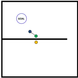
functions have cliffs. To see why, considerTWO-ROOM, a simple MDP presented in Figure 1. It
describes a world with two rooms connected by doorway. The agent can freely move through the
open space of the world but cannot go through the wall.1 A region in one room is marked as the
goal. The agent receives a reward of0when inside the goal and−1otherwise.
GOAL
Figure 1: The state space ofTWO-ROOM. There is a sample transition in the top room and state
near the sample in the bottom room
The optimal policy inTWO-ROOMis to navigate directly to the goal. Thus, the value of a state,s,
is decreasing in the length of the shortest path from it to the goal,dTR(s, g)(wheredTRdenotes
shortest-path metric). States that are physically close together but on opposite sides of the wall have
starkly different values. To solveTWO-ROOM, one must faithfully represent this steep drop in value
across the wall.
For KBRL to represent the value cliff, it must be run with a small bandwidth. Compensating for the resulting variance requires a large set of sample transitions, making the domain challenging for
KBRL. However, if we usedTR instead ofdEucas the metric in the mother kernel,TWO-ROOM
becomes easily solvable with a large bandwidth and small data set. Since the value function is
smooth with respect todTRwe can use large bandwidths with no risk of averaging across the wall.
We tried solvingTWO-ROOM with different combinations of bandwidth and metric, holding the
training set fixed 2. When running KBRL with a large bandwidth and the Euclidean metric, the
1For the purposes of discussion, assume the agent can move in any direction or choose to stay in place
Vertical Axis 0.0 0.2 0.4 0.6 0.8 Horizontal Axis 0.0 0.2 0.4 0.6 0.8 Value 70 60 5040 3020 10 64 56 48 40 32 24 16 8 Vertical Axis 0.0 0.2 0.4 0.6 0.8 Horizontal Axis 0.0 0.2 0.4 0.6 0.8 Value 10080 6040 20 0 105 90 75 60 45 30 15 0 Vertical-Axis 0.0 0.2 0.4 0.6 0.8 Horizontal-Axis 0.0 0.2 0.4 0.6 0.8 Value 100 80 60 40 20 105 90 75 60 45 30 15
Figure 2: Left to right:TWO-ROOM’s value function estimated withdEucandb=.06; withdEuc
andb=.01; and withdT Randb=.06
value cliff is completely smoothed out. The resulting policy has the agent attempt to walk through the wall. With a small bandwidth, KBRL finds the correct overall shape for the value function, but there are some ripples that appear as artefacts of the small bandwidth. The resulting policy has the
agent reach the goal on a path that zigzags around the shortest path. Running KBRL withdTRand a
large bandwidth produces the correct shape for the value function without any ripples. The resulting policy takes the agent to the goal along the shortest path.
The manifold of theTWO-ROOMstate space is a square with a line segment cut out of it. The value
function is smooth on the manifold but discontinuous in Euclidean space. Thus, using distance on
the manifold instead of Euclidean distance makes kernel regression work better. Domains like
TWO-ROOMhave been used to motivate representation discovery in parametric reinforcement learning,
most notably by Proto-Value Functions [10] which use the eigenfunctions of the manifold as a basis.
The discontinuity inTWO-ROOM’s value function comes from the local connectivity of the state
space, but local connectivity is not the only factor that affects value function smoothness. Consider,
for instance, a modification toTWO-ROOMwhere the wall is replaced by a region of low reward.
The agent can freely move through this region, but would get a better return by going around it. This modification removes the connectivity issues (the state space manifold is Euclidean space) but the value function still has the same discontinuity. Now consider a modification where the agent can jump over the wall if it has enough momentum. With this modification, two states that are close to
each other2and far from the wall can have very different values depending on whether the agent is
on a trajectory that can hurdle the wall. This modified version ofTWO-ROOMhas a value function
discontinuity that extends beyond the wall and no local information can help distinguish the states it
separates. NeitherdEucnordTRdo particularly well here.
The cases above show that a good metric must consider more than just local state space topology; it must also account for global dynamics and the reward structure of the MDP. In some sense, knowing the right metric requires already knowing the value function. The next section identifies the ideal metric and provides an algorithm for approximating it.
4 Value-Consistent Pseudometrics
KBRL uses kernel regression to approximate the Q-values of an MDP. It does this using kernels
of the formκa(s, s0) = ca·k(dEuc(s,s0)
b ), whereca is a normalizing constant. We are interested
in finding a new metricd0 to replaced
Euc in the regression. To keep things simple, we begin by
removing the reinforcement learning component of the problem and only considering regression.
2Note that here we are measuring distance in phase space. Two states are nearby if they have similar position
4.1 Transforming to Improve Regression
The problem statement of regression is as follows: given a set of training points,D={(xi, yi)|i=
1, . . . , n}, of point-value pairs withyi = f(xi)for somef : X → R, produce a functionf˜that
approximatesf well, for some measure of approximation quality.3
Regression with a kernel estimator [11] produces the estimatef˜(x) = Pik(b−1dEuc(x−xi))yi
P
ik(b−1dEuc(x−xi)) . In
Section 3, we found that replacingdEucwith a function that varies more closely withf can produce
better results. The function that varies most closely withfis the pseudometric4d∗
f(x, x0) =|f(x)−
f(x0)|. The diameter ofX underd∗
fdepends onf. We can remove this dependence using the scalar
µf =f∆maxX(−fdEucmin) to makedf(x, x0) =µfd∗f(x, x0), a pseudometric with the same diameter asdEuc.
df is the most natural choice for replacingdEucin the regression. We calldf thevalue-consistent
pseudometric (VCPM)forfonX.
Unfortunately, to usedfin the regression one would need to already knowf. Our workaround is an
iterative algorithm that interleaves steps of regression and metric learning to approximate the VCPM
forf onX. We start with an initial metricd0 =dEucand use the kernel estimator to produce an
estimatef1. We then usef1andd0to produce a new metricd1that corresponds to a representation
ofX wheref1 is smoother. We then used1in our kernel estimator to get a new estimatef2 and
repeat until the approximation stops improving.
The metricdi should be a relaxation of di−1 towardsdfi, the VCPM for fi on X. One way to
do this would be to choosedi(x, x0) = c0pdi−1(x, x0)2+α2dfi(x, x0)2, wherec0 is a diameter
preserving constant andα > 0 is a relaxation rate. Note that even thoughdfi is a pseudometric,
eachdiis guaranteed to be a valid metric onXbecause of the dependence ondi−1.
The effect of varyingαis discussed in the Appendix. The diameter preservingc0satisfies √1+1α2 ≤
c0 ≤1and is difficult to calculate exactly, so we assume the lower bound. Calculatingdfirequires
knowing the extrema offi, which are also difficult to compute but known to be bounded byymax
andymin; we use these bounds in place of the exact values. With these two heuristics, the metric will
underestimate some distances. Underestimating distances is equivalent to using a larger bandwidth, which is an acceptable trade-off for the performance improvement.
With these adjustments, our relaxation of the metric becomes
di(x, x0) = √ 1 1 +a2 s di−1(x, x0)2+ α∆(dEuc)fi(x)−fi(x 0) ymax−ymin 2 .
This relaxation can be viewed as a transform onX compressing it wherefiis flat and stretching it
wherefiis steep. This transform warps them-dimensionalXthroughm+idimensions in such a
way thatfibecomes smoother. For this reason, we call it aDimension-Adding Wrinkle-Ironing
Transform (DAWIT)[12]. Appendix A discusses the geometric interpretation of the transform in
more detail.
For reasons explained in Appendix A, we refer to “kernel regression augmented to learn a metric by DAWIT” as FDK. We are able to demonstrate a number of properties of FDK. We have experimental
evidence5that the best fit does not always occur in the limit. We also have proof that: in the limit
of infinite data and a bandwidth that shrinks at an appropriate rate, the metric learned converges to
the VCPM off onX; for a fixed bandwidth and dataset, iterating until convergence produces a
piecewise flat approximation off; the number of pieces in the piecewise flat approximation varies
inversely withb.
3We assume thatX is a compact, connected subset ofRm; and thatmaxiy
i=ymax6=ymin= miniyi.
From these assumptions it follows thatfhas distinct extrema onX; we refer to these asfmaxandfmin. We
refer to the diameter ofXunder metricdas∆X(d)
4d∗
f is a pseudometric because it doesn’t satisfyd∗(x, x0) =⇒ x=x0; in the supplementary matrials we
show that it is safe to used∗
f as a metric in kernel regression.
Claim In the limit of infinite data and a bandwidth that shrinks at an admissible rate6, performing
FDK to convergence with anyα >0will produce the VCPM of the function being approximated.
Proof. (sketch) We show this in two parts: First we show that repeatedly applying DAWIT with the same function produces a sequence of metrics converging to the VCPM for that function on its domain. Next, we use the convergence properties of kernel regression to show that FDK also possesses the property.
Part 1: The metric produced by DAWIT on iterationjsatisfies
dj(x1, x2) = s dj−1(x1, x2)2+α2µf2·(f(x1)−f(x2))2 1 +α2 = v u u td0(x1, x2)2 (1 +α2)j +α2µ2f ·(f(x1)−f(x2))2 j X i=1 1 (1 +α2)i.
Asj→ ∞, the term involvingd0goes to zero exponentially quickly and the summation on the right
converges toα−2. It follows that
lim
j→∞dj(x1, x2) =µf·(f(x1)−f(x2))
which is the VCPM forf onX.
Part 2: As the size of the dataset increases and the bandwidth decreases at an admissible rate, the first
estimate,f0, produced by kernel regression converges tof. It follows that the metricd1produced by
DAWIT converges to a relaxation towardsdf and subsequent iterations of FDK resemble DAWIT
repeated with the same function which, as we showed above, converges to the VCPM for the function on its domain.
The proof above shows that in the limit, FDK produces the pseudometric we identified as the ideal. Next we show the convergence properties of FDK by characterizing the fixed points of FDK. A
pseudometricdis afixed pointof FDK on datasetDif performing a round of DAWIT withdi−1=d
(andf˜ibeing the result of kernel regression withdi−1) producesdi=d.
Lemma A pseudometricdis a fixed point of FDK if and only if the functionf˜created by
perform-ing kernel regression usperform-ingdsatisfiesd(xi, xj) =µf˜|f˜(xi)−f˜(xj)|for allxi, xj∈D.
The proof of this lemma is some straightforward arithmetic substituting into the equation for
DAWIT; it is omitted in the interest of space. Next, we say a metric d is an attractive fixed
pointof FDK if there exists > 0 such that starting FDK from any pseudometricd0 satisfying
|d0(x, x0)−d(x, x0)| < for allx, x0 ∈ X, produces a sequence of converging tod. The set of
attractive fixed points is the set of pseudometrics to which FDK can converge.
Claim For a metric, dto be an attractive fixed point, the functionf˜resulting from doing kernel
regression withdmust be flat atxifor everyxi∈D.
Proof. (by contradiction) Assumedis an attractive fixed point of FDK for a given datasetDsuch
thatf˜is not flat at somexi ∈D. Assume WLOG thati= 1. f˜being non-flat atx1means in any
neighbourhood ofx1 there is somexsuch thatf˜(x) 6= ˜f(x1). Note that this can only happen if
d(x, x1)6= 0.
Given some, Letx∗ be a point such that: (x∗, f(x∗))∈/ D;d(x∗, x
1)< ; andf˜(x∗) 6= ˜f(x1).
Letd0be the pseudometric satisfyingd0(x, x∗) =d(x, x
1)for allxandd0(x, x0) =d(x, x0)for all
x, x0 6=x∗. The approximationf˜0 that results from usingd0 in kernel regression is identical tof˜
except atx∗, wheref˜0(x∗) = ˜f(x1)(sincex∗is not inDit has no influence over the regression). It
follows thatf˜0satisfies the constraints ford0to be a fixed point. Thereforeddoes not attractd0and
cannot be an attractive fixed point.
6An admissible shrinkage rate [1] is one where the bandwidth goes to zero but slowly enough (relative to
An implication of the claim above is that, in the limit, neighborhoods of points in the dataset get collapsed into singularities. The supplementary materials provide intuition about how this happens. In practice, we find that approximation error typically goes down then up, and the metric that mini-mizes it is found after just a handful of iterations. We also find that our augmented kernel regression
is very well suited for modelling discontinuities like the one inTWO-ROOM’s value function.
Ap-pendix B provides empirical data about fit quality.
Claim When performed using a kernel,k, with compact support having bandwidth,b < ∆X
c , for
some integer,c, FDK has an attractive fixed point withc+ 1singularities.
Proof. (by construction) Consider the datasetD ={(xi, yi)|i = 0. . . c}withxi =yi = i
pro-duced from a functionf : [0, c]→R. Letdbe the pseudometric such thatd(xi, xj) =dEuc(xi, xj)
for alli, j∈0, . . . , candd(x, x0) = 0for allx /∈ {x0, . . . , xc}.
First, we show thatd(x)is a fixed point. Letf˜be the function produced by kernel regression using
das the metric. Solving forf˜gives f˜(x) = Pjk(x, xj)yj. Because of the constraints on the
bandwidth,k(xi, xj) = 0for alli6=k, thusf˜(xi) =yi =xifor alliandf˜(x) =y0 =x0for all
x /∈ {x0, . . . , xc}.f˜is a line though allc+ 1points inD. By our lemma, this makes it a fixed point.
To show thatd(x)is attractive, we consider a new pseudometric that is a perturbation ofd. Letd0
be a pseudometric such that|d(x, x0)−d
0(x, x0)|< ∆(cX) −bfor all pairs of points(x, x0)inX.
Thef˜0that results from kernel regression usingd0satisfiesf˜0(x) = ˜f(x)because the perturbations
were made small enough that kernels centred on eachxi still do not overlap. During the metric
learning step, DAWIT produces the metricd1(x, x0) ∝
q
d0(x, x0)2+α2µ2( ˜f(x)−f˜(x0))2 =
p
d0(x, x0)2+ (αµd(x, x0))2. Note thatd1is a relaxation towardsd. Sinced1 satisfies the
con-straints we placed ond0, it follows thatd2, d3, . . ., are also relaxations todand that the sequence
{di}converges tod, makingdan attractive fixed point.
The proof above shows that the number of pieces in the piecewise flat approximation generated in the limit of FDK is inversely proportional to the bandwidth used. The proof can be extended to deal with kernels with infinite support.
4.2 Transforming to Improve Reinforcement Learning
Now that we have an extension of kernel regression capable of modelling a wider class of functions, we are ready to apply it to reinforcement learning.
It is tempting to think thatdVπ∗, the VCPM forVπ∗, is the ideal pseudometric. This is not the case;
dVπ∗ corresponds to an abstraction where all states with the same value are mapped to the same
abstract state. Such an abstraction discards information about the optimal action. What we need is an abstraction where only states with the same Q-values are mapped to the same abstract state.
We can produce such an abstraction by using the VCPMs for the Q-values.7 For each actionawe
wantκa(s, sai) = k(b
−1d
Qa(s,sai))
P
jk(b−1dQa(s,saj)). Note that we are using a different pseudometric in the kernel
for each action. Using the VCPMs for the Q-values corresponds to aQ∗-irrelevance abstraction;
it satisfiesΦ(s) = Φ(s0) =⇒ Qπ∗
(s, a) = Qπ∗
(s0, a)∀asincekΦ(s)−Φ(s0)k = 0 ⇐⇒
dQaQ(s, s0) = 0∀a ⇐⇒ Qπ∗(s, a) =Qπ∗(s0, a)∀a. Acting optimally with respect to Q-values
in aQ∗-irrelevance abstraction results in optimal behaviour in the ground MDP [13].
Now that we have identified the desired abstraction, we can construct an algorithm to approximate it. As we did for regression, we start from the Euclidean metric and iteratively estimate the Q-values (with KBRL) and update our metrics (with DAWIT). Algorithm 1 describes the process.
In practice we found that it was rarely worth doing more than five iterations of DKBRL. There is one important detail that is worth mentioning; the algorithm reuses the same dataset on each iteration
Algorithm 1DAWIT-KBRL 1: procedureDKBRL(S0, b) 2: da 0 ←dEuc∀a 3: i←0 4: repeat 5: Qi←KBRL(S0, b, di) 6: fora∈Ado 7: da i+1←DAWIT(dai, Qai) 8: end for 9: i←i+ 1
10: untilPolicy stops improving.
11: returnQi−1
12: end procedure
because the problem formulation is to learn from a batch of sample transitions. Were we free to collect fresh data between iterations, we would want the sampled points to be uniformly distributed with respect to the latest metric. Doing so is necessary for KBRL’s correctness guarantees. Uniform coverage with the learned metric is equivalent to concentrating samples in the regions of state space where the Q-values are steep, which is sensible because that is where the Q-values tend to be poorly
approximated. In TWO-ROOM, sampling uniformly from the transformed space corresponds to
choosing more samples along the wall.
We ran DKBRL onTWO-ROOMwith a large bandwidth (b=.06) to see if it could identify the wall.
The results were successful; DKBRL was able to learn a metric that separated states on opposite sides of the wall. To visualize the metric, we sampled some points in the state space, calculated all-pairs-shortest-paths, and performed multidimensional scaling [14] to get a 2D projection. Figure 4.2 shows the projection resulting from the metric for one action; the projections for the other actions were similar.
0.8 0.6 0.4 0.2 0.0 0.2 0.4 0.6 0.8 First Principal Component
0.6 0.4 0.2 0.0 0.2 0.4 0.6
Second Principal Component
0.8 0.6 0.4 0.2 0.0 0.2 0.4 0.6 0.8 First Principal Component
0.4 0.3 0.2 0.1 0.0 0.1 0.2 0.3 0.4
Second Principal Component
1.0 0.8 0.6 0.4 0.2 0.0 0.2 0.4 0.6 First Principal Component
0.3 0.2 0.1 0.0 0.1 0.2 0.3
Second Principal Component
Figure 3: DKBRL opening the wall inTWO-ROOMover three iterations. Points are colored by
ground truth value (red=high, blue=low). After the first iteration (left) a rift has started to form, by the third iteration points are completely separated by value.
5 Results
We start by demonstrating our approach work on Mountain-Car, a simple reinforcement learning domain that allows us to easily visualize the value function and gain insight about how DKBRL works. We then present our main results: performance improvements on the more challenging Acrobot and PinBall domains.
5.1 Mountain-Car (proof-of-concept)
Mountain-Car is a two dimensional MDP [6] modelling a car with a weak motor attempting to
drive out of a valley.8 The car is not powerful enough to escape directly and must build up energy
by rolling back and forth. Mountain-Car’s value function has a discontinuity that goes in a spiral
through the state space, separating states where the car has enough energy to make it up the hill on its current roll from states that require an additional back and forth.
Velocity 0.0 0.2 0.4 0.6 0.8 Position 0.00.2 0.40.6 0.8 Value 120 100 80 60 40 20 0 105 90 75 60 45 30 15 0 Velocity 0.0 0.2 0.4 0.6 0.8 Position 0.00.2 0.40.6 0.8 Value 160 140 120 100 80 60 40 20 160 140 120 100 80 60 40 20 Velocity 0.0 0.2 0.4 0.6 0.8 Position 0.00.2 0.40.6 0.8 Value 100 80 60 40 20 105 90 75 60 45 30 15
Figure 4: (Left to right) Mountain-Car’s value function; the value function as approximated by
KBRL withdEucandb=.09; and the approximation after four iterations of DKBRL withα= 1.
Our representation discovery algorithm allows KBRL to capture the discontinuity remarkably well. It is also able to find the correct value for the bottom of the hill (note the axes). Nonetheless, because Mountain-Car is such an easy problem, there is little difference in the policies induced by KBRL’s and DKBRL’s value function approximations. What matters for solution quality is not the value function approximation error, but that the best action gets assigned the highest Q-Value.
5.2 Acrobot
Acrobot is a four-dimensional MDP [6] modelling a two-link robot resembling a gymnast on a high bar. The gymnast can actuate at the waist and must raise its feet above some height by swinging back and forth. The acrobot domain has a value function discontinuity that resembles that of Mountain-Car.
For our experiments, we collected 15000 sample transitions per action, with start points selected to uniformly cover the reachable state space. We generated a solution from the transitions using KBRL then performed two iterations of DKBRL. We conducted three sets of experiments, one for
each bandwidth:.03,.06, and.09. To account for the effects of random sampling we repeated each
experiment 6 times and averaged the results. For each run, we choseα =.5because that worked
well in our regression experiments in the supplementary materials.
0 100 200 300 400 500 Steps 0.0 0.2 0.4 0.6 0.8 1.0
Fraction Reaching Goal
Solution qualities, b=.03 KBRL DKBRL, Iter 1 DKBRL, Iter 2 0 100 200 300 400 500 Steps 0.0 0.2 0.4 0.6 0.8 1.0
Fraction Reaching Goal
Solution qualities, b=.06 KBRL DKBRL, Iter 1 DKBRL, Iter 2 0 100 200 300 400 500 Steps 0.0 0.2 0.4 0.6 0.8 1.0
Fraction Reaching Goal
Solution qualities, b=.09
KBRL DKBRL, Iter 1 DKBRL, Iter 2
Figure 5: (Top to bottom) The average solution qualities for the three experiments. The plots show the cumulative distributions of steps-to-goal. The standard errors are drawn on the graph.
Figure 5 shows the average solution qualities for the three sets of experiments. Each plot shows cumulative distribution of the number of steps it took to reach the goal state from 230 start states selected to uniformly cover the reachable state space. Note that the plots are the averages of the 6 experiments performed at each bandwidth and that the standard-errors are drawn on the graph but are hard to see because they are so small.
We now point out the salient features of the graphs. In roughly 30% of states, the agent is near the
end of a trajectory that reachs the goal (i.e. <50steps from the goal). In these easy states all the
solutions perform the same. The solution quality in the remaining 70% of states is what matters.
For the size of our dataset,b = .03is too small; KBRL undersmooths and produces a bad initial
amplifies the noise and produces even worse policies. When we chose the more reasonableb=.06, KBRL produces a good policy. One round of DKBRL is able to improve on this, slightly shortening the steps-to-goal for 65% of all states. The next round of DKBRL, however, is counter-productive,
failing to reach the goal from 10% of states. When b = .09 the effects of oversmoothing the
discontinuities starts to show for KBRL. The graph is much slower to rise than whenb =.06. A
round of DKBRL offers a sizeable improvement for 60% of states. The second round of DKBRL offers no additional improvement.
Since DAWIT is designed to solve the problem of oversmoothing at discontinuities, we would expect DKBRL to improve over KBRL when the bandwidth is large. This is what appears to be happening here, but it is difficult to say for sure because the graphs are so similar. Because the discontinuity in Acrobot’s value function is not along a decision boundary, improving the fit there does not do much for solution quality. In the next subsection, we consider a domain where discontinuities correspond to decision boundaries.
5.3 PinBall
PinBall is a four-dimensional MDP that models a ball navigating through a maze towards a goal [16]. The ball is dynamic, and bounces off obstacles; the five actions allow the ball to either stay in place or accelerate slightly along one of the compass directions. PinBall is particularly challenging because it is easy to get stuck on a wall while rounding a corner. Furthermore, some of the obstacles are so thin that they are hard to detect from the sample transitions.
We conducted our tests on one of the maps that came with the open source code.9 We had to make
two modifications to the domain: first, we fixed a bug that allowed the ball to pass through walls under some circumstances and second, we increased the time discretization threefold so as to reduce the amount of data needed to solve the problem.
For this set of experiments, we collected 20000 sample transitions per action uniformly from the reachable state space. We then passed the samples through KBRL followed by two iterations of
DKBRL. We did this four times each at bandwidths.04,.07and.09 keeping the relaxation rate
fixed atα=.5. The resulting steps-to-goal cumulative distributions are showin in Figure 6.
0 100 200 300 400 500 Steps 0.0 0.2 0.4 0.6 0.8 1.0
Fraction Reaching Goal
Solution qualities, b=.04 KBRL DKBRL, Iter 1 DKBRL, Iter 2 0 100 200 300 400 500 Steps 0.0 0.2 0.4 0.6 0.8 1.0
Fraction Reaching Goal
Solution qualities, b=.07 KBRL DKBRL, Iter 1 DKBRL, Iter 2 0 100 200 300 400 500 Steps 0.0 0.2 0.4 0.6 0.8 1.0
Fraction Reaching Goal
Solution qualities, b=.09
KBRL DKBRL, Iter 1 DKBRL, Iter 2
Figure 6: The average solution qualities for PinBall forb=.04,.07, and.09respectively.
For our chosen sample size,b =.04is near the optimal value for KBRL. KBRL produces its best
solution there and performing iterations of DKBRL makes the performance worse. We suspect that
this happens because the value function approximation produced by KBRL has large ripples10which
then get amplified by DAWIT making the fit worse.
When we raise the bandwidth tob=.07, the effects of oversmoothing kick in and the performance
of KBRL plummets. Here DKBRL is able to counteract the bias resulting from oversmoothing and
produce a solution comparable to the one produced by KBRL atb = .04. The resulting average
for the second iteration of DKBRL withb =.07is similar to that of KBRL withb =.04, but the
variance is smaller.
Finally, when we raise the bandwidth to.09, the oversmoothing of KBRL is too much for DAWIT
to undo. DKBRL manages to improve upon the initial solution, but not by much.
9The code is available athttp://www-all.cs.umass.edu/˜gdk/pinball/. We used the map
pinball-easy.cfg
10In our discussion ofTWO-ROOMwe note that performing KBRL with small bandwidths produces value
These experiments suggest that the key merit of DKBRL is that it can reduce the need for bandwidth tuning by allowing for near optimal solutions to be found over a wider interval of bandwidths.
6 Related Work
The method closest to ours for non-parametric regression is Metric Learning for Kernel Regression (MLKR) [17], which finds the Mahalanobis metric best suited for performing kernel regression. Using Mahalanobis distance is equivalent to applying a linear transform to the input space. Linear transforms are not powerful enough to smooth out discontinuities and would offer little help
ap-proximatingTWO-ROOM’s value function. Predictive Projections [18] uses an approach similar to
MLKR for dimensionality reduction in parametric reinforcement learning.
Other related algorithms are ST-ISOMAP [19] and Action Respecting Embedding [20], which use modified nearest-neighbors algorithms to discover and unroll the manifold containing the data. These algorithms have not been applied to RL. They would be well suited for learning a repre-sentation for problems where value function discontinuity arises from local state space topology. Existing representation discovery algorithms for parametric RL have largely focused on modifying the parametric representation of the value function itself. One early approach was Proto-value func-tions (or PVFs) [10], which uses nearest neighbors on the sample transifunc-tions to discover the manifold of the state space and uses the eigenfunctions of the graph Laplacian as a basis for representing the value function. PVFs, along with the related diffusion wavelet approach [21], focus on the topol-ogy on the state space and offer little additional leverage when discontinuities arise from the MDPs reward structure. Another parametric approach is the use of Bellman-error basis functions (BEBF) [22], which are learned basis functions that represent the Bellman error in previous approximations. BEBFs are similar in spirit to the technique we present in this paper; however, they are used as basis functions in a linear value function approximation architecture.
We do not attempt to produce experimental results comparing our algorithm to any of the techniques presented above. They attempt to address problems that are related to, but distinct from, what DAWIT is designed for and there is no meaningful comparison that can be made.
7 Conclusion and Future Work
Representation discovery, which has so far been investigated primarily in parametric approaches to reinforcement learning, is a promising area in the context of nonparametric approaches. A partic-ularly interesting next step would be to explore an online version of DKBRL to that samples new points for coverage in the transformed space. The correctness guarantees of KBRL require sampling points uniformly from the domain. Sampling uniformly from our transformed domain is equivalent to concentrating samples near value function discontinuities in the state space, which is desirable since that is where the value function is hardest to represent.
Acknowledgments
We would like to acknowledge the help of Leslie Kaelbling and Tom´as Lozano-P´erez through every step of this project. We would also like to thank Tommi Jaakkola for a conversation about kernels.
References
[1] Dirk Ormoneit and ´Saunak Sen. Kernel-based reinforcement learning. Machine learning, 49(2-3):161– 178, 2002.
[2] Dirk Ormoneit and Peter Glynn. Kernel-based reinforcement learning in average-cost problems. IEEE
Transactions on Automatic Control, 47(10):1624–1636, 2002.
[3] Andr´e da Motta Salles Barreto, Doina Precup, and Joelle Pineau. Reinforcement learning using kernel-based stochastic factorization. InAdvances in Neural Information Processing Systems 24, pages 720–728, 2011.
[4] Andr´e da Motta Salles Barreto, Doina Precup, and Joelle Pineau. On-line reinforcement learning using incremental kernel-based stochastic factorization. InAdvances in Neural Information Processing Systems 25, pages 1493–1501, 2012.
[5] Andr´e MS Barreto, Doina Precup, and Joelle Pineau. Practical kernel-based reinforcement learning. Technical report, Laboratrio Nacional de Computao Cientfica, May 2014.
[6] Richard S Sutton and Andrew G Barto.Reinforcement learning: An introduction. MIT press, 1998. [7] Martin L Puterman. Markov Decision Processes: Discrete Stochastic Dynamic Programming, volume
414. John Wiley & Sons, 2009.
[8] Justin A Boyan. Least-squares temporal difference learning. InProceedings of the 16th International
Conference on Machine Learning, pages 49–56, 1999.
[9] Gavin A Rummery and Mahesan Niranjan. On-line Q-learning using connectionist systems. University of Cambridge, Department of Engineering, 1994.
[10] Sridhar Mahadevan and Mauro Maggioni. Proto-value functions: A Laplacian framework for learning representation and control in Markov decision processes.Journal of Machine Learning Research, 8(10), 2007.
[11] Jacqueline K Benedetti. On the nonparametric estimation of regression functions. Journal of the Royal
Statistical Society, pages 39:248–253, 1977.
[12] Dawit Zewdie. Representation discovery in non-parametric reinforcement learning. Master’s thesis, MIT, Cambridge MA, 2014.
[13] Lihong Li, Thomas J Walsh, and Michael L Littman. Towards a unified theory of state abstraction for MDPs. InInternational Symposium on Artificial Intelligence and Mathematics, 2006.
[14] Joseph B Kruskal. Multidimensional scaling by optimizing goodness of fit to a nonmetric hypothesis.
Psychometrika, 29(1):1–27, 1964.
[15] Brian Tanner and Adam White. RL-Glue : Language-independent software for reinforcement-learning experiments.Journal of Machine Learning Research, 10:2133–2136, September 2009.
[16] George Konidaris and Andrew G Barto. Skill discovery in continuous reinforcement learning domains using skill chaining. InAdvances in Neural Information Processing Systems 22, pages 1015–1023, 2009. [17] Kilian Q. Weinberger and Gerald Tesauro. Metric learning for kernel regression. In11th International
Conference on Artificial Intelligence and Statistics, 2007.
[18] Nathan Sprague. Predictive projections. InInternational Joint Conference on Artificial Intelligence, pages 1223–1229, 2009.
[19] Odest Chadwicke Jenkins and Maja J Matari´c. A spatio-temporal extension to ISOMAP nonlinear di-mension reduction. InProceedings of the 21st International Conference on Machine Learning, page 56, 2004.
[20] Michael Bowling, Ali Ghodsi, and Dana Wilkinson. Action respecting embedding. InProceedings of the
22nd International Conference on Machine Learning, pages 65–72. ACM, 2005.
[21] Sridhar Mahadevan and Mauro Maggioni. Value function approximation with diffusion wavelets and Laplacian eigenfunctions. InAdvances in Neural Information Processing Systems 18, pages 843–850, 2006.
[22] Ronald Parr, Christopher Painter-Wakefield, Lihong Li, and Michael Littman. Analyzing feature genera-tion for value-funcgenera-tion approximagenera-tion. InProceedings of the 24th International Conference on Machine
A Transforming For Improved Fit
This section provides a different interpretation of DAWIT, the metric learning algorithm presented in Section 4.1. We start by introducing Fit-Improving Iterative Representation Adjustment (FIIRA), a function approxi-mation framework under which DAWIT falls. We then present an intuitive explanation of the rational behind DAWIT.
A.1 Fit-Improving Iterative Representation Adjustment
The problem statement of curve-fitting is as follows: given a set of training points, D = {(xi, yi) |i =
1, . . . , n}, of point-value pairs withyi = f(xi)for some functionf : X → R, produce a function f˜to
approximatefwell, for some measure of approximation quality.
A regressor,r, is a procedure for creating fits from some space of functions,Fr. Iffis not well approximated
by any function inFr, the fit generated byris guaranteed to be poor. One way to fix to this problem is to
transform the domain off and work in a space wheref iswell approximated. Choosing such a transform requires prior knowledge or assumptions aboutf.
Since we are not in a position to make assumptions aboutf, we wish to infer a transform directly from the data. Our idea for doing so, is to passDto the regressor, then use the approximation produced to infer a transform
Φof the domainXsuch thatfonΦ(X)is better approximated byFr. Algorithm 1 describes the framework
for doing this. The procedure takes as input a dataset,D; a regressor,REGR; and a transform generator,T F.
Algorithm 2Fit-Improving Iterative Representation Adjustment
1: procedureFIIRA(D, REGR, T F)
2: Φ0←x7→x .Identity transform
3: D0←D
4: i←0
5: repeat
6: f˜i+1←REGR(Di) .Perform regression
7: Φi+1←T F( ˜fi+1, Di) .Produce transform
8: Di+1← {(Φi+1(x), y)|(x, y)∈Di} .Update the dataset
9: i←i+ 1
10: untilfi˜ ≈fi−˜ 1 .Or until best fit attained
11: returnx7→fi˜(Φi−1(x))
12: end procedure
A formal analysis of the properties of FIIRA for a general regression scheme and transform generator is outside the scope of this paper and is left for future work. What follows is a discussion of FIIRA for the special case where the regressor is a local-averaging kernel smoother and the transform generator is DAWIT.
A.2 Dimension-Adding Wrinkle-Ironing Transform
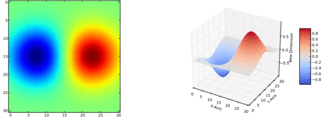
In the paper we claim that the metric created by DAWIT corresponds to a transform that warps the state space through a higher dimension. We now elaborate on that.
Consider a transform generator that, given a functionf with domainX, returns a transformΦwhich maps everyx∈Xtohx|f(x)i(the bar represents concatenation).ΦstretchesXintod+ 1dimensions in a way that pulls apart points that differ in value (See Figure 6).
After the transformation, the distance between two pointsaandbin the domain offbecomes
kΦ(a)−Φ(b)k=p
ka−bk2+ (f(a)−f(b))2.
Note thatkΦ(a)−Φ(b)kvaries more closely with|f(a)−f(b)|than doeska−bk.
The transformΦdoes what we want, but it has two problems; it is sensitive to the scale off, and it can change the diameter ofX. We fix these problems by normalizingfbyαµf andΦ(X)byc0(as defined in the main
body of the paper).
With these two changes,Φmaps them-dimensional vector,x = (x1, . . . , xm)to them+ 1-dimensional
x0= (c
0x1, . . . , c0xm, c0αµf·f(x)). The distance metric that corresponds to the final form of this transform
is
kΦ(a)−Φ(b)k=c0 q
ka−bk2+α2µ2
0 5 10 15 20 25 30 0 5 10 15 20 25 30 X-Axis 0 5 10 15 20 25 300510Y-Axis 1520 2530 New Dimension 0.5 0.0 0.5 0.8 0.6 0.4 0.2 0.0 0.2 0.4 0.6 0.8
Figure 7: The figure on the left is a heatmap of some function with a two-dimensional domain. The areas in red are where it attains a high value and the ones in blue are where it attains a low value. The figure on the right shows the two-dimensional domain stretched through three dimensional space in such a way that separates points that differ in value. The red areas are pulled up and out of the page while the blue ones are pushed down and into the page. Distances in this transformed space correspond to the metric produced by DAWIT.
When we substitute forµf andc0, this equals the metric produced by DAWIT; hence the name
“dimension-adding” VCPM relaxation. We refer to kernel regression augmented to use DAWIT as FDK because it is a FIIRA approach combiningDAWIT andKernel-regression.
A.3 How DAWIT works
Kernel-regression produces function estimates using local averaging. As a result, the approximation is good where the target function, f, is linear and bad where it has high curvature. It follows that the curvature of the estimate,h(x), is correlated with the approximation error. Thus, we can infer where the approximation likely to be poor just by looking at the approximation.
We use this insight to construct a transform of the input domain,X, into a space whereh(and thus alsof) are smoother. Our transform warps themdimensionalX into them+ 1dimensionalX0in such a way that
its diameter is preserved but some neighborhoods grow or shrink depending on the slope ofh. The metric produced by DAWIT corresponds to distances inX0.
Letfbe the unit step function and letX= [−1,1]. One iteration of kernel regression produceshresembling a sigmoid. hattains its maximum slope nearx = 0. Performing DAWIT withhproduces a metric,d, that stretches the area aroundx= 0(i.e. d(−, ) >2∗, for small||) and squashes the regions nearx = 1
andx=−1. The pointx= 0itself may get moved closer tox= 1orx= −1, but that does not matter. What matters is that on the next round of regression the region aroundx= 0is magnified, making it easier to pinpoint where the discontinuity lies. This magnification is analogous to using a smaller bandwidth atx= 0. One can see now why we call the transform ”wrinkle-ironing”. The discontinuity in the step function resembles a crease on an article of clothing. Repeated application of the transform smooths this and similar value cliffs much like a hot iron passing over a wrinkly shirt.
A.4 Value Consistent Pseudometric
In the main body of the paper, we claimed that using the VCPM as a valid metric in kernel regression was theoretically sound. We now justify that claim.
When viewed under the lens of a FIIRA approach, the VCPM can be seen as coming from a transformΦ∗that
satisfieskΦ∗(x)−Φ∗(x0)k=µ
f|f(x)−f(x0)|. A transform that satisfies this property isΦ∗(x) =µff(x).
Under this interpretation, we are mapping each point to its scaled value and performing kernel regression to fit a line. Only points with identical values get mapped to the same point by the transform. SinceΦ∗is a safe to
use before doing regression, performing kernel regression with the VCMP for the function being approximated cannot cause problems.
B Graphs
This section contains graphical demonstrations of the convergence properties of FDK. It starts by showing how FDK converges to a piecewise flat approximation when modelling a line. It goes on to show the FDK fits generated for some datasets.
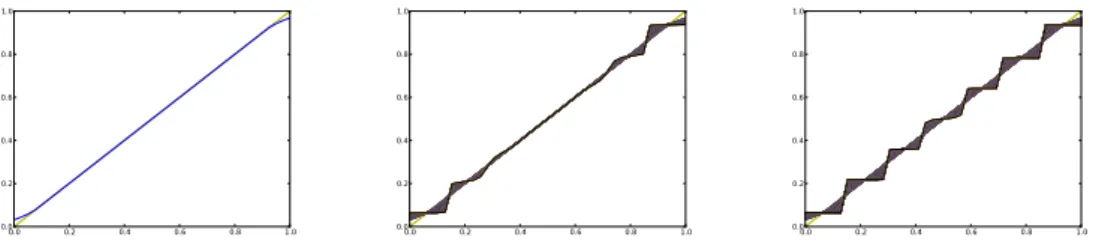
0.0 0.2 0.4 0.6 0.8 1.0 0.0 0.2 0.4 0.6 0.8 1.0 0.0 0.2 0.4 0.6 0.8 1.0 0.0 0.2 0.4 0.6 0.8 1.0 0.0 0.2 0.4 0.6 0.8 1.0 0.0 0.2 0.4 0.6 0.8 1.0
Figure 8: How FDK converges to a piecewise flat approximation when attempting to fit a line. The
figure on the left shows the first fitf˜0in blue. Note how the fit is biased at the boundaries. This bias
gets amplified over the next several iterations of FDK (middle). The end result is the piecewise flat approximation on the right. If we had used a smaller bandwidth there would have been more pieces in the piecewise flat approximation.
When fitting a line, the approximation error increases with every iteration. For most functions, however, the error goes down for a few iterations before going up. The following figures show the result fitting some select functions with different combinations of parameters.
Below we have included plots that show approximation quality of FDK for some select datasets. The plots on the left show the dataset (scatter plot), the kernel regression fit (dotted blue line), the best FDK fit obtained (solid red line), and the piecewise flat function to which FDK converges for the value ofαthat produced the best fit (green pluses). The plots on the right show how the approximation error changes as a function of iteration number for different values ofα. Approximation error is measured as the sum of squared errors, normalized so that the fit produced by the vanilla kernel regression has unit error. Note how low the error dips and how few iterations it takes to get there.
0.0 0.2 0.4 0.6 0.8 1.0 1.0 0.5 0.0 0.5 1.0 FDK approximation with b=0.1 Kernel Smoother Fit Best FDK Fit FDK Limit Input Data 0 5 10 15 20 25 30 35 40 Iteration 0.0 0.2 0.4 0.6 0.8 1.0 Error FDK approximation error alpha=0.25 alpha=0.5 alpha=1.0 alpha=2.0 0.2 0.4 0.6 0.8 0 2 4 6 8 10 FDK approximation with b=0.1
Kernel Smoother Fit Best FDK Fit FDK Limit Input Data 0 5 10 15 20 25 Iteration 0.2 0.3 0.4 0.5 0.6 0.7 0.8 0.9 1.0 Error FDK approximation error alpha=0.25 alpha=0.5 alpha=1.0 alpha=2.0
0.0 0.2 0.4 0.6 0.8 1.0 1.0 0.5 0.0 0.5 FDK approximation with b=0.15 Kernel Smoother Fit Best FDK Fit FDK Limit Input Data 0 5 10 15 Iteration20 25 30 35 40 0.2 0.4 0.6 0.8 1.0 1.2 1.4 1.6 Error FDK approximation error alpha=0.25 alpha=0.5 alpha=1.0 alpha=2.0 0.0 0.2 0.4 0.6 0.8 1.0 0.6 0.4 0.2 0.0 0.2 0.4 FDK approximation with b=0.1
Kernel Smoother Fit Best FDK Fit FDK Limit Input Data 0 5 10 15 20 25 Iteration 0.0 0.2 0.4 0.6 0.8 1.0 1.2 Error FDK approximation error, b=0.1 alpha=0.25 alpha=0.5 alpha=1.0 alpha=2.0