A Thesis submitted to the University of Sheffield
for the degree of Doctor of Philosophy in the Faculty of Engineering
by
T. J. Rogers
Department of Mechanical Engineering University of Sheffield
It is impossible to properly thank all the people who have helped and supported me through the course of this PhD in this short section. They know who they are and I am truly grateful. There are, however, a few people whose support I would like to highlight and to whom I would like to extend my thanks.
First and foremost, I could not have wished for a better place to conduct this research than as part of the Dynamics Research Group. The DRG is a very special place, full of inspiring people; who, every day, push me to be better than I thought I could be. I owe a special thanks to Dr Lizzy Cross, who has been a wonderful supervisor, who has stopped me getting lost in many rabbit holes, and who has taught me how to write. I wish to thank Dr Graeme Manson for his advice and guidance, and for many interesting conversations about bread. Finally, I count myself very lucky to have had input from Prof. Keith Worden; who has been a solid sounding block, on a number of occasions.
I am also grateful to Ramboll Energy for their support of this work. In particular my thanks go to Ulf Tygesen who has been able to offer fantastic guidance regarding the aims of the offshore industry and insight into current industry practice. I wish to thank Prof. Thomas Sch¨on for hosting me at Uppsala university for a very productive two weeks. Along with the rest of his team, especially Andreas Lindholm; his input was invaluable in completing the work found in Chapter 5.
My thanks go to Paul for being a great friend, for deciphering papers with me, and for helping generate more ideas than we can work through. Among the many friends I have in the DRG, I am especially lucky to have spent time with and worked with Ramon, Nikos, and Lawrence; for each of whom I am very grateful.
Finally, to Ruth, you are my best friend; I could not have done this without you. You have kept my priorities straight, encouraged me more than I deserve, and always been there for me. For all of this, and more, I am eternally thankful.
sented and discussed
• The problem of system identification for SHM is handled in a Bayesian manner within both Gaussian Process, state-space mod-els, and Bayesian clustering frameworks
• The best practice for Gaussian Process models is discussed with reference to their application in SHM
• It is shown how the kernel of a GP can encode prior belief about the physical process
• Novel use of population based optimisation of Gaussian Process hyperparameters is shown to outperform the usual gradient based approach
• The importance of model choice in Gaussian Processes is shown for an SHM example
• The Gaussian Process NARX model is presented, highlighting some of the challenges in its implementation
• A novel comparison of uncertainty propagation techniques for GP-NARX is made
• The problem of lag selection in GP-NARX is discussed and con-trasted with parametric NARX models
• The modelling of wave loading — a key unknown — on offshore structures is attempted
• The current standard model, the Morison equation, receives a Bayesian treatment and is contrasted with a black-box approach • The applicability of Gaussian Process models to wave loading
(including GP-NARX) is explored and discussed
• The novel use of particle Gibbs is shown for system identification problems in structural dynamics
• It is shown how ancestor sampling and particle rejuvenation can aid Particle Gibbs methods in structural dynamics
• The identification of a Duffing oscillator highlights the effectiveness of the method — especially in the presence of high noise
• The Gaussian Process Latent Force Model is introduced for the problem of load estimation in structural dynamics
• It is shown that this can be efficiently rewritten as a linear state-space model
• This is used to perform joint input-state-parameter estimation in an operational modal analysis setting
• A Dirichlet process model is introduced for online Bayesian clus-tering of SHM data
• The technique removes the need to pre-collect a training dataset or add information on expected damage conditions
• Random Projection is exploited to allow online unsupervised dimensionality reduction
• A framework which allows for incorporation of prior knowledge of damage states leads to a flexible and practical model
Within the offshore industry Structural Health Monitoring remains a growing area of interest. The oil and gas sectors are faced with ageing infrastructure and are driven by the desire for reliable lifetime extension, whereas the wind energy sector is investing heavily in a large number of structures. This leads to a number of distinct challenges for Structural Health Monitoring which are brought together by one unifying theme — uncertainty. The offshore environment is highly uncertain, existing structures have not been monitored from construction and the loading and operational conditions they have experienced (among other factors) are not known. For the wind energy sector, high numbers of structures make traditional inspection methods costly and in some cases dangerous due to the inaccessibility of many wind farms. Structural Health Monitoring attempts to address these issues by providing tools to allow automated online assessment of the condition of structures to aid decision making.
The work of this thesis presents a number of Bayesian methods which allow system identification, for Structural Health Monitoring, under uncertainty. The Bayesian approach explicitly incorporates prior knowledge that is available and combines this with evidence from observed data to allow the formation of updated beliefs. This is a natural way to approach Structural Health Monitoring, or indeed, many engineering problems. It is reasonable to assume that there is some knowledge available to the engineer before attempting to detect, locate, classify, or model damage on a structure. Having a framework where this knowledge can be exploited, and the uncertainty in that knowledge can be handled rigorously, is a powerful methodology. The problem being that the actual computation of Bayesian results can pose a significant challenge both computationally and in terms of specifying appropriate models. This thesis aims to present a number of Bayesian tools, each of which leverages the power of the
Bayesian paradigm to address a different Structural Health Monitoring challenge. Within this work the use of Gaussian Process models is presented as a flexible nonparametric Bayesian approach to regression, which is extended to handle dynamic models within the Gaussian Process NARX framework. The challenge in training Gaussian Process models is seldom discussed and the work shown here aims to offer a quantitative assessment of different learning techniques including discussions on the choice of cost function for optimisation of hyperparameters and the choice of the optimisation algorithm itself. Although rarely considered, the effects of these choices are demonstrated to be important and to inform the use of a Gaussian Process NARX model for wave load identification on offshore structures.
The work is not restricted to only Gaussian Process models, but Bayesian state-space models are also used. The novel use of Particle Gibbs for identification of nonlinear oscillators is shown and modifications to this algorithm are applied to handle its specific use in Structural Health Monitoring. Alongside this, the Bayesian state-space model is used to perform joint input-state-parameter inference for Operational Modal Analysis where the use of priors over the parameters and the forcing function (in the form of a Gaussian Process transformed into a state-space representation) provides a methodology for this output-only identification under parameter uncertainty. Interestingly, this method is shown to recover the parameter distributions of the model without compromising the recovery of the loading time-series signal when compared to the case where the parameters are known.
Finally, a novel use of an online Bayesian clustering method is presented for performing Structural Health Monitoring in the absence of any available training data. This online method does not require a pre-collected training dataset, nor a model of the structure, and is capable of detecting and classifying a range of operational and damage conditions while in service. This leaves the reader with a toolbox of methods which can be applied, where appropriate, to identification of dynamic systems with a view to Structural Health Monitoring problems within the offshore industry and across engineering.
1 Introduction 1
1.1 SHM: A Probabilistic Challenge? . . . 2
1.2 The Bayesian Approach . . . 4
1.3 SHM as System Identification . . . 8
1.4 SHM for Offshore . . . 9
1.5 Contribution of This Thesis . . . 10
2 Implementation of Gaussian Process Models for SHM 13 2.1 The Gaussian Process Model . . . 16
2.1.1 Assessing GP Performance . . . 23
2.2 Learning Gaussian Processes for SHM . . . 26
2.3 Kernel Selection in Engineering . . . 31
2.3.1 Kernel Selection Techniques . . . 37
2.4 Choice of Cost Function . . . 39
2.4.1 Mean-Squared Error . . . 39
2.4.2 z – Score . . . 40
2.4.3 Negative Log Marginal Likelihood . . . 42
2.4.4 Predictive Probability . . . 43
2.5 Hyperparameter Optimisation . . . 44
2.5.1 Effect of Optimisation Scheme . . . 46
2.5.2 Results . . . 49
2.6 Discussion . . . 61
3 Handling Dynamic Data with Gaussian Process NARX Models 63 3.1 The GP-NARX Model . . . 64
3.2 Handling Uncertainty in GP-NARX Predictions . . . 66
3.2.1 Fixed Variance . . . 68
3.2.2 Monte-Carlo Sampling . . . 68
3.2.3 Moment Matching Uncertainty Propagation . . . 69 v
3.3 Comparison of UP Methods in GP-NARX . . . 72
3.4 Lag Selection in GP-NARX . . . 82
3.5 Discussion . . . 83
4 Wave Load Modelling 87 4.1 White-Box Modelling . . . 89
4.2 Black-Box Modelling . . . 96
4.2.1 Cross-validation Training of GP-NARX Models . . . 101
4.3 Discussion . . . 107
5 Particle-Gibbs for Nonlinear System Identification 111 5.1 The Bayesian State-Space Model . . . 113
5.2 Methods for Nonlinear State Space Models . . . 115
5.2.1 Modifications to the Kalman Filter . . . 115
5.3 Sequential Monte Carlo . . . 117
5.4 Particle Gibbs . . . 121
5.4.1 Ancestor Sampling . . . 122
5.4.2 Particle Rejuvenation . . . 123
5.5 Identification of a Duffing Oscillator . . . 125
5.5.1 Modelling of the Duffing Oscillator using SMC . . . 127
5.5.2 The Role of Particle Rejuvenation . . . 133
5.6 Discussion . . . 135
6 State Space Models for Coupled Load-Parameter Identification 139 6.1 Continuous-Discrete LGSSMs . . . 143
6.2 The Latent Force Approach . . . 144
6.3 Application to Operational Modal Analysis . . . 152
6.4 Results . . . 153
6.4.1 LFM With Known System Parameters . . . 154
6.4.2 OMA With The LFM . . . 156
6.5 Discussion . . . 159
7 Online Bayesian Clustering for Damage Detection 161 7.1 Finite Gaussian Mixture Models . . . 166
7.2 Dirichlet Process Gaussian Mixture Models . . . 167
7.3 Online Inference in the SHM Context . . . 173
7.3.1 Hyperparameter Selection . . . 175
7.3.2 A Suggested Decision Making Process . . . 176 vi
7.4.2 Z24 Bridge Data . . . 191
7.5 Discussion . . . 196
8 Conclusions and Future Work 199 8.1 Gaussian Processes for SHM . . . 200
8.2 State-Space Modelling for SHM . . . 202
8.3 Dirichlet Processes for SHM . . . 204
8.4 Future Work . . . 204
8.5 The Outlook for Offshore . . . 207
Appendix 213
A Linear Gaussian State-Space Models 213
B Details of 5th Order Runge-Kutta Scheme 217
Bibliography 218
Introduction
As the title of this thesis reflects, this document and body of work represents a stepping stone in an ongoing pursuit by some (the author included) to revolutionise the way engineering is done in the 21st century. Society is in the midst of what some would term the “data revolution” [1], where the ongoing digitisation of everyday life is giving rise to ever larger collections of data. This is a key factor in driving what has been dubbed the “fourth industrial revolution” [2] in an attempt to characterise the rapid changes happening in the way the world operates. This transformation could be considered by some — possibly correctly — to be merely the next set of buzzwords driving this generation’s “bubble”. However, this new-found availability of large datasets and (possibly more importantly) computing power is changing how engineering problems are tackled.
Classical engineering, where experiments are performed on a small scale in a labora-tory and empirical relationships are deduced (more often than not linear or log-linear relationships), is no longer the primary focus of research. Nor is the application of these simple models the main driver in engineering design and production, instead the use of Finite Element or Multi-body Physics models has become the mainstay of engineering design. More recently, developments in the application of machine learning models, in which the need for physical insight is often removed (or possibly ignored), have led to new approaches to solving engineering problems.
A field which has been heavily influenced by the explosion in machine learning seen over the last two/three decades is that of Structural Health Monitoring (SHM).
2 1.1. SHM: A PROBABILISTIC CHALLENGE?
SHM is the process of collecting data from a structure of interest; in some manner using this to learn about the condition of that structure; and to aid and inform the process of making an engineering decision regarding its operation. Although the use of “physical” models to understand the condition of structures has been and continues to be an active area of research in the SHM community [3, 4], the use of machine learning or statistical methodologies has become a mainstay of many SHM analyses [5, 6].
It is the author’s opinion that the engineering community is faced with a philosophical dilemma; will, as ever more data become available, research be able to uncover a hidden order in systems of interest, allowing perfect prediction of the behaviour of engineering structures? The experience of the author is that, rather than this being the case, data only highlights the disorder in the world around us. That is, the future of engineering will not be defined by the removal of uncertainty but rather defined by how it is understood and handled. This motivates the need to investigate methodologies which are capable of representing and incorporating uncertain data. Invariably, this involves the adoption and adaptation of methods, developed by statisticians and later machine learning researchers as a groundwork for rigorous handling of uncertainty.
1.1
Structural Health Monitoring: A
Probabilis-tic Challenge?
The task of SHM is often approached by introducing Rytter’s Hierarchy [7], which breaks down the overarching question of what is the condition of a structure into a number of sub-tasks, of increasing challenge. These being,
1. Detection 2. Localisation 3. Assessment 4. Prediction
This was extended in Worden and Dulieu-Barton [8] to a five level problem which is used now:
1. Detection — is there damage present?
2. Localisation — where has damage occurred?
3. Classification — what type of damage is present?
4. Quantification — what is the severity/extent of the damage?
5. Prognosis — what is the remaining useful life of the structure?
Hopefully, some of the advantages of changing the mindset of an engineer, when approaching these problems, will become clear as they are discussed here and throughout this thesis.
The problem of detection is a good place to start, not only is it the first challenge in the hierarchy but it is the simplest to understand from a probabilistic perspective. Detection is concerned with identifying whether or not a structure is damaged; see the fundamental axioms of SHM for a definition of this [9]. This has commonly been approached as a problem with a binary outcome, “yes there is damage” or “no there isn’t”. Here the task of damage detection becomes a deterministic one-class classification problem [10]. This can be thought of as giving the outcome as a ‘crisp’ or ‘hard’ label. There are many examples of this type of damage detection approach within SHM [11–17]. The alternative view on this problem would be to consider, not whether a structure is damaged or not, but instead to attempt to quantify a probability of damage which can be propagated into a decision framework, for example see [18, 19].
This assessment of different approaches can be continued up the hierarchy, for instance, considering the classification problem as estimating the likelihood of membership to each class [20–23]. Although, the added information from the probabilistic estimation of classes can often be neglected by condensing this to the single most likely label. Likewise, the localisation problem can be considered in terms of identifying the most likely place damage may have occurred [24] or even a distribution over possible damage locations. The quantification problem can be considered to be a problem of estimating the distribution over possible damage extents [25]. Finally, this approach to the prognosis problem becomes to estimate the distribution over the remaining useful life of a given structure [26–29].
4 1.2. THE BAYESIAN APPROACH
1.2
The Bayesian Approach
Since Rev. Thomas Bayes introduced a new manner in which to view problems of probability in the late 18th century, the Bayesian approach has been a competitor to traditional frequentist statistics. Before considering the mechanics of a Bayesian approach to uncertain problems, it is useful to consider an example which highlights some of the benefits of a Bayesian outlook. Say a teacher decides to conduct a survey of a subset students in a class of two hundred in order to receive feedback. They ask twenty students if they are happy or unhappy with the course. Only six of these students reply that they are happy with the course and the teacher is put out — as any good instructor would be — assuming (as a frequentist) that the expected satisfaction in the class is only 30%. Over a coffee, they are advised by their Bayesian colleague to revisit their analysis from a different standpoint.
The colleague explains that, as a Bayesian, they think it is dangerous to accept only a small sample as representative of a population. They suggest that instead it might be useful to consider including any other knowledge that might be available. It transpires (this being a somewhat manufactured example), that there has recently been a survey of student satisfaction across the whole course (this class included). From this, it was possible to build a probability distribution of what percentage of students would be happy in a randomly selected class1. The two teachers now have
everything needed to conduct a Bayesian analysis of the student satisfaction2.
Breaking this down, the building blocks of Bayesian inference are having some model of the likelihood of the object of interest. In this case, the likelihood is simply the ratio of satisfied students to the total number of students surveyed. This is combined with some prior information which is encoded as a probability distribution. When choosing a prior it is important that it can accurately reflectexpert beliefs; or, if not possible to do this, encode a lack of belief — in other words it formalises uncertainty before any data are collected. It is important that the prior has support over an appropriate domain, this means that samples from the prior will exist only in the domain (and across the entire domain) where the variable of interest exists. For this problem it is known that the object being modelled is the fraction of the students that are satisfied with the course, therefore, it does not make sense to have an outcome
1Formally, this prior is described by a Beta distribution with parametersa= 70 andb= 30 2Since the yes/no survey is a Bernoulli process and the prior is a Beta distribution, the posterior
0 20 40 60 80 100 Precentage of Satisfied Students 0 0.002 0.004 0.006 0.008 0.01 Probability
(a) Sample of twenty
0 20 40 60 80 100
Precentage of Satisfied Students 0 0.002 0.004 0.006 0.008 0.01 0.012 0.014 Probability (b) Sample of 180
Figure 1.1: Plots of the prior (blue) and posterior (green) distributions for student satisfaction given the survey of twenty students (a) and 180 students (b).
less than zero or greater than one. The Beta distribution is appropriate here since its support is [0,1] — i.e. all numbers drawn from it will lie in the interval [0,1]. By following a Bayesian analysis, it was possible for this teacher to compute the distribution over the student satisfaction given this survey of a subset of students. In Figure 1.1(a), the prior distribution is shown in blue and the posterior distribution is shown in green. The posterior encodes the distribution over the percentage of satisfied students, given the prior knowledge, which comes from knowing the overall course satisfaction, and the information from the survey of the subset. It can be seen that, since the survey includes only a small number of students it is not able to move the posterior very far from the prior — certainly it would fill the teacher with more confidence than accepting the frequentist result of 30% satisfaction!
Still concerned, the first teacher decides to extend the survey to 180 students (a much larger proportion of the class). Out of these students 110 indicate that they are satisfied with the class, which equates to∼61% in the frequentist viewpoint. If a Bayesian analysis is followed, the new posterior distribution (based on the same prior as before) is shown in Figure 1.1(b). Here, it can be seen that the prior belief has been able to moderate the effect of the small sample size from before and the results are remarkably similar. It should also be noted that as more data are collected the posterior distribution will tend towards the likelihood, that is that the frequentist solution is recovered in the limit of infinite data — which is where it is guaranteed. But, how is the object of interest, the posterior distribution, computed? It is known
6 1.2. THE BAYESIAN APPROACH
that the posterior distribution is a probability distribution over the variable of interest (in this case the proportion of students who are satisfied). The posterior distribution is best thought of as the updated belief after observing some data. This is just the rigorous combination of what a modeller believes before any observations are made (the prior) and the information contained in the observed data (the likelihood). Computing this requires the use of Bayes’ theorem which is simple to derive given two key identities in probability theory.
The first is the relationship between joint and conditional probabilities, the chain rule of probability,
p(a, b) = p(a|b)p(b) =p(b|a)p(a) the second is the law of marginalisation which is written
p(a) =
Z
p(a|b)p(b) db
Importantly, the chain rule for probabilities can be applied in either order, this makes the derivation of Bayes theorem trivial:
p(a, b) = p(b, a) (1.1a)
p(a|b)p(b) = p(b|a)p(a) (1.1b)
p(a|b) = p(b|a)p(a)
p(b) (1.1c)
This shows that Bayes’ theorem is just an application of the chain rule of probability where, sometimes, this will be written with the denominator as an integral using the law of marginalisation property. Introducing some terminology, the distribution
p(a|b) is referred to as the posterior; p(b|a), the likelihood; p(a), the prior; and
p(b), the marginal. In terms of computation it can be more helpful to consider Bayes theorem as written below.
p(a|b) = R p(b|a)p(a)
p(b|a)p(a) da (1.2)
The problem in practical application of Bayesian methods is also more apparent when the theorem is written in this form. It is usually possible to write down a
likelihood for the data, this involves deciding on a probabilistic model for the system. It is also possible to elicit a user’s prior belief, although care should be taken on how to do this [30, 31]. The hard part of the implementation is computing the marginal integral that is the denominator of Equation (1.2). In many cases this will not be available in closed form, this is why many Bayesian analyses use a seemingly very restricted set of prior distributions — usually in the exponential family. The choice of priors where the marginal, and therefore the posterior, can be computed in closed form for the given likelihood allows much faster analysis. These priors are referred to as being conjugate to the likelihood.
In a large number of cases, it will not be possible to ensure conjugacy in the model — even when solving a simple problem such as linear regression in a fully Bayesian manner it is not possible to obtain a closed form solution. In these situations it is possible to target the posterior directly via some numerical approximation, popular tools include Markov Chain Monte Carlo (MCMC) [32, 33] where the posterior is approximated by point masses generated from a Markov Chain or variational inference where the form of the posterior is approximated by a known distribution which can be computed in closed form [33].
The real beauty in the Bayesian analysis is that it conforms to a very human understanding of the world. That is, the belief that events don’t happen purely in isolation. When encountering new situations, humans can draw on knowledge that they already have to help guide their belief given a small amount of available information. It is this ability to incorporate prior belief that helps humans generalise problem solving tasks across different domains (one of the great challenges in machine learning). It also helps explain how, as humans, two people can witness the same event but come to very different conclusions. To use a slightly topical example, when there is a change of government followed by an increased economic output, it is prior belief that leads one group of people to say this is a long term effect from the previous administration compared to another group which accredit this to the fresh policies of the new administration. As more data become available the strength of a given person’s prior belief is actually revealed through their posterior (current) belief. Clearly, this discussion is in some ways facile, but an exposition of the philosophical basis for a Bayesian vs. frequentist standpoint is beyond both the scope of this thesis and quite possibly the capabilities of the author! If this discussion is of interest, most good texts introducing Bayesian inference include at least a passing discussion on the topic, see [33–35].
8 1.3. SHM AS SYSTEM IDENTIFICATION
As becomes apparent when using these methods, the stumbling block in Bayesian inference is not normally a philosophical one but a practical one. Despite the theory existing to build complicated hierarchical models which can represent multi-layered engineering systems, lack of available knowledge and computing power can restrict the usability of these. As greater amounts of computing power become readily available it opens up new possibilities for the use of these highly complex Bayesian models — the challenge is not to become absorbed by the modelling and lose sight of what the model is trying to represent. It is important, therefore, to continue discussions about how this approach can add benefit to engineering analyses and be applied in a rigorous and usable manner.
1.3
Structural Health Monitoring as System
Iden-tification
The task of Structural Health Monitoring is closely related to that of system identifi-cation — if a system could be fully identified and modelled then prognosis within a Structural Health Monitoring framework would be possible. A perfect model of a system is not attainable; yet, through more rigorous and powerful system identifica-tion, many of the challenges in Structural Health Monitoring can be reduced. Here the task of system identification is considered in its broadest sense, to understand the behaviour of dynamical systems given some observations — and of course, being Bayesian, any available prior knowledge. This can include the task of parameter estimation but also extends to building models which can make predictions either over unknown outputs or to recover unknown inputs.
The central aim of system identification is to be able to recreate the behaviour of a system through some model which can be implemented and from which inferences can be made about the system. For uses in SHM by inferring the parameters of the model (more usefully the distributions over the parameters) changes in the system can be observed — this is the main tenet of model updating approaches to SHM [4]. In a data driven manner, the ability to predict the behaviour of a system accurately and with quantified uncertainty allows the use of these predictions for the modelling of damage mechanisms or for detection of changes in the system behaviour without the requirement for a valid physical model.
As a simple example, one of the hardest challenges in SHM is that of prognosis. A user may be interested in the prognosis for a structure given its fatigue damage accrual. If the response of the structure could be identified and predictions could be made regarding the expected strain across the structure then this could be used in a predictive fatigue analysis. Additionally to this, it would be necessary to identify the loading on the system which gives rise to this response in order to quantify the amount of expected damage in the future. This is obviously a significant undertaking in practice but, assuming that the system could be fully identified in terms of its response and prediction of expected loading, the task of prognosis for SHM becomes merely inspecting the outputs of the model. Hopefully this highlights the intrinsic link between the desire to implement robust SHM systems and the task of performing system identification.
1.4
Structural Health Monitoring for Offshore
The offshore energy industry was one of the earliest investigators into the application of Structural Health Monitoring on commercial structures. The nature of the offshore environment led to a need for structural assessment when traditional inspections were either not possible, or were very costly. Early examples of the use of vibration measurements include [36, 37]. As part of this, output only techniques for under-standing a structure’s behaviour were also developed from a system identification standpoint and operational modal analysis [38] remains a key tool for offshore. The increased interest in SHM was motivated by the need to prove the structural integrity of these structures as they age and to do so in a cost effective manner. This has led to the development and integration of Risk & Reliability based inspection models where the inspection schedule is driven (at least in part) by measured data from the structure. The approach of Risk & Reliability attempts to model the risk as a probability of failure and when this exceeds a certain level to drive a cost effective intervention, see [39, 40]. Bayesian approaches to the problem have also been considered, for example pre-posterior decision theory [41, 42], or the use of Bayesian networks [43]. Although presented in literature, the current uptake of these methodologies in industry is unclear.
Although many of these technologies were developed for the offshore oil & gas industry, the growth of the offshore wind energy market is also driving development
10 1.5. CONTRIBUTION OF THIS THESIS
of monitoring systems [44] — and related technologies. Due to the obvious influence of the condition of rotating machinery on the operation of the wind turbine, there has been investigation into the application of Condition Monitoring for offshore wind [45], this is a closely related field to that of SHM and it shares many of the challenges. In fact, there has been a substantial body of research into monitoring of wind turbine bearings and gearboxes [46–50].
The question is, what makes offshore a challenging (and therefore more interesting) environment in which to perform SHM? The nature of working with offshore structures is such that, many of the open problems in SHM are encountered at one time. These are systems in environments with severely changing operational conditions, which operators are unable to quantify [17, 51–53]; where the structural models are uncertain [54, 55] and based upon output only analyses [56] and modal expansion techniques [57, 58]. Alternatively, direct fatigue load analysis could be considered which requires estimation of the input loads [59–63]. These problems are further complicated by the inherent nonlinearity in the system, both from the nonlinear fluid structure interaction [64] and from foundation conditions [65–68]. These factors contribute to a highly uncertain environment with significant challenges for both system identification and for SHM due to the high number of unknowns and confounding influences. It is also an environment where there is tangible cost benefit for implementation of SHM strategies due to the high cost of maintenance and inspection. This motivates continuing research into the application of emerging technologies for SHM of offshore structures.
1.5
Contribution of This Thesis
The work of this thesis aims to introduce and utilise some potentially powerful technologies which, having been developed in the statistics and machine learning communities, can now bring significant value to engineering. The work focuses on the application of these methods to SHM problems. Before explaining these individual methods it has been necessary to present a short introduction to SHM from a probabilistic perspective and to introduce the Bayesian paradigm on which the methods used in this thesis are built. Chapter 2 introduces the Gaussian Process model as a Bayesian nonlinear regression tool for SHM. Following this Chapter 3 contains research into the practical application of these models, how the Gaussian
Process can be used robustly within an engineering context. This includes the use of the Gaussian Process NARX model for handling dynamic data. Chapter 4 contains a demonstration of the application of these Gaussian Process models for the problem of load identification on offshore structures — this is dominated by the wave loading. Chapters 5 and 6 present the use of Bayesian state-space models for both nonlinear system identification and then the use of a Latent Force Model as an alternative approach to the load estimation problem. Finally, an online Bayesian approach to damage detection and classification is introduced in Chapter 7. This approaches the problem of SHM from a different perspective to the preceding chapters — that is treating it as a classification problem rather than a regression problem. This is followed by a number of conclusions which can be drawn from this work and suggestions on how the results seen here might motivate future research.
Implementation of Gaussian
Process Models for SHM
Highlights:
• The best practice for Gaussian Process models is discussed with reference to their application in SHM
• It is shown how the kernel of a GP can encode prior belief about the physical process
• Novel use of population based optimisation of Gaussian Process hyperparameters is shown to outperform the usual gradient based approach
• The importance of model choice in Gaussian Processes is shown for an SHM example
Within SHM, a large number of problems can be considered to be a regression task. This can be used in an indirect way, for instance, predicting some unknown variable in a system such as loading or response — a popular subset of this is sometimes referred to as virtual sensing [69, 70]. Alternatively, regression can be used directly within an SHM system to predict damage location or damage extent, e.g. the length of a fatigue crack. Various approaches are available to do this; for many years the use of linear regression models has been prevalent. This includes models that are
14
“linear in the parameters”, such as a linear regression (e.g. the Morison equation for simplified calculation of wave loading) which can occur on a log-log scale as in common in fatigue analysis. Linear regression models can be insufficient to fully capture the behaviour of physical systems, in fact, within engineering many processes are inherently nonlinear, e.g. the true wave loading on offshore structures.
When the physical process of a system is known, it can be possible to define a nonlinear model parametrically. These models are normally computationally more demanding since many systems do not have closed form solutions — a pertinent example is the Navier-Stokes equations which would allow calculation of wave loading on a structure, but are famously not solved in closed form, for more information see Temam [71]. The approximation of these systems numerically is possible and is considered viable in certain circumstances [72]. The major challenge is when it is not possible to write down, exactly, the equations which govern a given system. This may be due to lack of specific knowledge about some aspect of the system, such as the boundary conditions. It could, however, be due to lack of understanding of the physics driving the problem. The alternative being that, the system is comprised of very many, individually complicated, systems such that it would be impossible for a user to fully describe its physical behaviour.
When this is the case, a model form has to be chosen which will be used for the regression. The problem is that, while there is a single truly linear model for a given set of inputs and outputs, there is an infinity of nonlinear models — that is the set of all possible basis functions. The model selection problem remains one of the biggest challenges in engineering where the physics of the system is not fully known. Many approaches restrict the model form to a set of basis functions — transformations of the input variables. For example, these bases could be chosen to be polynomial or Fourier [20]. The problem remains to choose the appropriate bases from a given set, “which polynomial terms will give the best model?”. If fitting a polynomial regression model to a finite number of points, one will notice that increasing the number of bases will reduce the error when minimising the sum square error to fit the parameters (or if there are more parameters than there are data points the model is unsolvable). However, when new data arrive, this model will perform very badly. This is due to the function in the model being far more complicated than the function driving the process. This is commonly referred to as overfitting.
These types of basis function models are referred to as parametric models. This reflects the fact that, as more nonlinear functions are modelled, the number of bases
increases and with that, the number of parameters. There is one parameter associated with each basis, e.g. in a quadratic polynomial model there are three parameters, one for the quadratic term, one for the linear term, and one for the constant. It is this growing number of parameters that causes problems in overfitting and model selection. To combat this, approaches have been developed that broadly fall into two categories:
1. Cross-validation — leaving out subsets of data from the parameter estimation process and minimising the error on these sets, the limit of this being leave-one-out cross-validation where the size of the set is one data point.
2. Regularisation — introducing additional terms to the cost function used for parameter estimation which penalise more complex models to introduce a trade off between model fit and model complexity.
Both of these approaches are valuable in fitting parametric models but require comparison of many model forms and different model orders. This can be a difficult and computationally expensive task. It is desirable, therefore, to look for models where the model order (number of bases) does not need to be specifieda priori. Such a model exists in the Gaussian Process (GP).
Gaussian Processes (GPs) present a flexible non-parametric Bayesian prior over functions [73, 74]. The GP model can be explained in a number of ways, the two most popular approaches are to either motivate the extension of the problem of Bayesian linear regression or to consider the GP as the limit of a multivariate Gaussian distribution as the dimensionality tends to infinity. The view of the GP as an extension of Bayesian linear regression is a more intuitive starting point in most cases, and this will be presented here briefly. More thorough discussions can be found in a number of textbooks [74–76].
The Gaussian process model as already achieved some attention in the engineering community. Particularly within SHM [53, 77–79]. This includes the investigation into the use of a GP as an emulator for a more expensive computer model [80, 81]. Most of this work has been to directly apply models developed within the machine learning community, for wider adoption, consideration of their implementation specifically for engineering warrants further investigation. This thesis aims to frame many of the results from the GP community within engineering problems and also to consider
16 2.1. THE GAUSSIAN PROCESS MODEL
additional difficulties that an engineer might encounter and how these might be overcome.
2.1
The Gaussian Process Model
When introducing the Gaussian process model, it is useful to start with the simplest Bayesian regression model — a linear regression model with noise only present on the output. For this, a parametric equation can be written down; where the aim is to determine the distribution over the weights,w, which best describe the relationship between the column vector of inputs,x, and the output,y. In the case of a standard one-dimensional linear regression, the weights represent the slope and offset of the line.
f(x) = xTw
y=f(x) +ε
(2.1)
The model is formed such that it aims to model some target y as a function of an observed certain set of inputs x corrupted by an additive noise ε. The function is assumed to be an additive linear combination of the inputs weighted by some vector of weights w. As is commonplace, the noise in the model can be assumed to be Gaussian distributed with zero mean and a known variance, σn2, such that
ε ∼ N(0, σ2n). This assumption ensures that a solution to the model is available in closed form — this approach is coincidently equivalent to a Tikhonov or L2
regularisation [20] when computing a deterministic model. By construction, it is possible to write down the likelihood of the output for a given input.
p(y|x,w) =N xTw, σn2 (2.2)
Usually, there will be more than one data point available so the vector of inputs,x, be-comes a matrix of inputs,X, where this matrix is assembled by stacking observations across the rows,X ={x1, . . . ,xN}, for N observed points. Therefore, the outputs
for each observation, y = {y1, . . . , yN}, have a joint likelihood, p(y|X,w). Since
the noise is generated i.i.d. (independently identically distributed) this likelihood can be computed as the product of the individual likelihoods. It should be noted at
this point that the offset in the linear model is introduced by extending the input matrix with a column of ones, this provides a more compact notation by not needing to state this offset explicitly.
p(y|X,w) = N Y i=1 p(yi|xi,w) =N XTw, σ2nI (2.3)
In the case of the Bayesian linear regression, the first object of interest is the posterior distribution over the weights given the observed data, D = {X,y}, which is the distribution p(w|X,y) =p(w| D). The likelihood has already been defined by the form of the model, Equation (2.3). It only remains to specify a prior distribution as the marginal can be computed via the integral of the likelihood and the prior. Since inference is performed over the weights in the model, w, the prior must be specified for these. It is sensible to choose this prior to be a multivariate Gaussian since this ensures conjugacy with the likelihood (which allows a closed form solution) and has the required support for the weights (i.e. the distribution admits all real numbers as samples). The prior is parameterised such that it is zero mean with a specified covariance, p(w)∼ N(0, Σw). Using these two definitions and the marginalisation
property, the posterior distribution over the weights can be written down.
p(w|X,y) = p(y|w, X)p(w)
p(y|X)
= R p(y|w, X)p(w)
p(y|w, X)p(w)dw
(2.4)
If this is calculated, due to the choice of prior and likelihood, the posterior distribution of the weights is also Gaussian and the mean and covariance can be expressed in a closed form, by completing the square.
p(w|X,y)∼ N σn−2Z−1Xy, Z−1
Z =σn−2XXT+ Σ−w1 (2.5)
This gives the distribution of the weights in the model based on the data which has currently been observed, both inputs and outputs, assuming that there is noise only present on the output and that noise is Gaussian distributed, zero mean with
18 2.1. THE GAUSSIAN PROCESS MODEL
known variance. This is normally, however, not the final quantity of interest. Instead, models are used to perform inference on new data; to make some prediction of a new output value given a new input value based on the data that has previously been observed. To do this, the posterior predictive distribution,p(y?|x?, X,y) needs to
be calculated. This is the distribution over a new test outputy? given a new test
input pointx? and the previously observed data. Again, the marginalisation identity
allows this to be computed, the weights of the model are marginalised out leaving the distribution over this new output based only on the previously observed data.
p(y?|x?, X,y) = Z p(y?|x?, X,y,w)p(w|X,y)dw =N σn−2xT?Z−1Xy, xT?Z−1x? (2.6)
This may appear to be a restrictive model; it is known that many functional relation-ships exist, in SHM and across engineering, which are not linear — in fact it is often hypothesised that nothing is truly linear. This, however, is not as significant a barrier as might be expected. It is possible to transform the inputs using a basis function expansion, here instead of only considering an inputx, some transformation,φ(x), of this input can instead be fed into the model. A common basis, which could be used, is a polynomial basis where the inputs are generated as polynomials transforms of the input, for example if a one dimensional input,x, is observed this can be related to the output via a quadratic rule where φ(x) = [x0, x1, x2]. Here there is a separate weight over each term in the basis function expansion, and the transform fits into the Bayesian linear regression model as before if we assume thatx=φ(x). Likewise, for multiple observations the same basis function expansion can be applied giving a matrix of transformed inputs, Φ (X), where the expansion of every input is stacked row-wise. Analysis proceeds as before and the predictive posterior can be written down, substituting φ(x?) forx? and Φ (X) for X.
p(y?|φ(x?), X,y) = Z p(y?|φ(x?),Φ (X),y,w)p(w|Φ (X),y)dw =Nσn−2φ(x?) T Z−1Φ (X)y, φ(x?) T Z−1φ(x?) Z =σn−2Φ (X) Φ (X)T+ Σ−w1 (2.7)
After some rearrangement, it can be shown that this distribution can be expressed only in terms of dot products of the input space, φ(x). This allows the relationship
to be expressed through a reproducing kernel Hilbert space — that is the covariance kernel. The covariance kernel (also covariance function) is a function which computes the covariance between any two inputs,k(x,x0). This is commonly referred to as the ‘kernel trick’ and allows definition of the inner product matrix directly through the Reproducing Kernel Hilbert Space. The kernel trick appears across machine learning and statistics literature, for example, it is also used in the support vector machine [20].
Moving to a kernel representation of the relationship, of the inputs; under certain conditions, is equivalent to using an infinite basis function set, thereby removing the need to specify a basis function set. The GP can be interpreted as a prior over a family of functions where that family is the one described by the covariance kernel, this will be discussed further in Section 2.3. From this is it possible to define the GP fully in terms of its mean and covariance function despite being a flexible nonlinear model. One powerful interpretation of a GP is as the infinite dimensional extension of a multivariate Gaussian distribution.
f(x)∼ GP(m(x), k(x,x0)) (2.8)
When a finite number of training data pairs are observed, D={xi, yi}Ni=1, as before
the inputs can be stacked into a matrix, X, and the outputs into a vector, y. At this point the data is distributed according to a multivariate Gaussian, where the mean is given by the mean function of the GP and the covariance is defined by the covariance function between every data point, K(X, X) — the elements of this matrix Ki,j =k(xi,xj). Since the observations are corrupted with some Gaussian
white noise of a known variance a diagonal term must be added to the covariance matrix, the magnitude of which is the noise varianceσ2n. The distribution is as shown in Equation (2.9).
y∼ N m(X) , K(X, X) +σn2I (2.9)
When a new point is observed, where the inputs are known, but inference needs to be made over the output, this forms a joint distribution with the training data.
20 2.1. THE GAUSSIAN PROCESS MODEL " y f? # =N " m(X) m(x?) # , " K(X, X) +σ2nI K(X,x?) K(x?, X) K(x?,x?) #! (2.10)
Here, inference is made over the underlying latent function,f?, although by adding
noise this can be extended to inference over values which will be observed,y?. This
can be useful if using the prediction in a damage detection scenario. In order to recover the predictive distribution overf?,p(f?|x?, X,y), it is necessary to condition
f? on the training data — this is equivalent to the conditioning of a joint multivariate
Gaussian distribution — which gives rise to the following equation.
p(f?|x?, X,y) = N(E[f?] , V[f?]) E[f?] =m(x?) +K(x?, X) K(X, X) +σn2I −1 (y−m(X)) V[f?] =K(x?,x?)−K(x?, X) K(X, X) +σ2nI −1 K(X,x?) (2.11)
Equation (2.11) is the key equation in GP regression models which allows the expectation and variance of the prediction to be expressed in closed form based solely on the relationship between the training and testing data through the kernel and the mean functions. Commonly, the mean function is considered to be zero so the equations can be rewritten removing these.
p(f?|x?, X,y) = N(E[f?] , V[f?]) E[f?] =K(x?, X) K(X, X) +σ2nI −1 y V[f?] =K(x?,x?)−K(x?, X) K(X, X) +σ2nI −1 K(X,x?) (2.12)
Presented with the maths, it can be easy to miss the simplicity of what the GP is trying to achieve. Here, only the GP with a zero mean function is considered but, as shown, the extension to a parametric mean is trivial. Under the GP prior, before any data have been observed, the predictions of the model will be zero for every input with a variance equal to the signal variance of the kernel this is demonstrated in Figure 2.1.
Figure 2.1: The Gaussian Process prior with a zero mean function is a Gaussian distribution across the output at every input with zero mean and variance equal to the signal variance of the kernel,σ2f
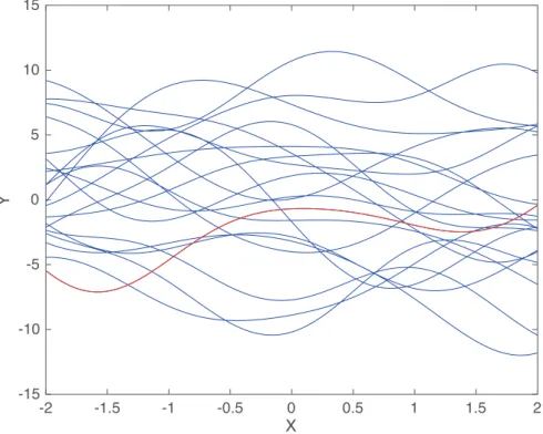
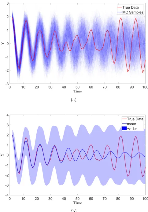
the GP in terms of the confidence intervals can obscure the actual understanding of what these represent. Since the GP is a distribution it is possible to draw random samples from it, as shown in Figure 2.2. These random draws, instead of being merely random variables, are in fact random functions over the input space. It can be seen that, under the prior, different functions drawn from the GP will be similar in terms of the functional form, which is defined by the kernel, but may not be good representations of the data which is being modelled, shown in red. It is also possible to make draws from the posterior distributions to create realisations of the possible functions that could have given rise to the observed data or possible functions for some new set of inputs.
The Bayesian nature of the GP is revealed as more data are added to the training process — if it was not obvious in the construction of the model! Figure 2.3 shows the effect of adding progressively more points to the training dataset. As more points are added the posterior (prediction) is more influenced by previously observed points and less resembles the prior. The effect could be described by the prediction being pinched around or pinned to the training data points. As the model is used to predict
22 2.1. THE GAUSSIAN PROCESS MODEL -2 -1.5 -1 -0.5 0 0.5 1 1.5 2 X -15 -10 -5 0 5 10 15 Y
Figure 2.2: The interpretation of the GP as a prior over functions becomes clear when draws are made from the prior, here the lines is blue are all possible functions under the prior in Figure 2.1 with the red line being the true function.
further away from the observed training points the prediction returns to the prior and the confidence intervals increase, indicating that the model is less certain making predictions at those points.
One might find it helpful to imagine the prior distribution as a large (infinite) number of snakes wriggling around in a child’s play tunnel (which represents some confidence interval), at points where data are observed it can be thought of as restricting the diameter of this tunnel to force all of the snakes together. Here the snakes are analogous to the potential latent functions, where the metaphor falls down is that the support of the predictive distribution at every point is across the whole real line and, therefore, the snakes should not be strictly constrained by the tunnel. Therefore, any real value is a potential sample from the distribution, however, many values become highly unlikely quickly as is normal in a Gaussian distribution. Likewise the functions exist over the whole real line — in the standard GP — for the inputs and (thankfully...) no snake is infinitely long.
(a) GP with one training point (b) GP with five training points
(c) GP with twenty training points (d) GP with forty training points
Figure 2.3: Figures showing posterior predictions of the GP as more training points are added. Discrete data observations are shown by crosses where the ones highlighted in red are used in the training process.
In the example shown, by the time forty training points are added to the GP, Figure 2.3(d), the functional form of the training data is very well captured and the model can successfully interpolate across that part of the input space, X. It is clear that the model is still unable to extrapolate; since there is no data to guide the GP the prediction returns to the prior. In fact, even if the model is interpolating, e.g. Figure 2.3(b) around X = 0, if the input space is not well covered in the training set, the GP is unable to make a confident prediction as to the expected output.
2.1.1
Assessing GP Performance
It is important to consider what is meant by a “good fit” in the context of a GP model. The general approach to quantifying model fit in SHM has been to consider some form of mean-squared error. This works well in a deterministic setting but
24 2.1. THE GAUSSIAN PROCESS MODEL
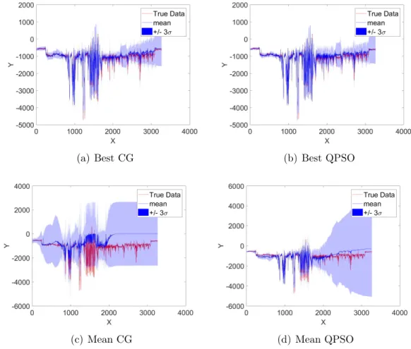
Figure 2.4: Plots of Gaussian process predictions for a function with training points shown in red and test points in grey, the prediction both in the mean, solid blue line, and the 3σ confidence intervals shaded in blue. Although all solutions it can be seen that the fit of some models is more desirable.
fails to quantify the quality of a probabilistic fit. Fuentes [50] discusses the uses of likelihoods as a model quality metric in SHM, here, the author agrees this is a sensible approach. It is possible to shown that the GP can be given a universal kernel such that it can fit a target function arbitrarily well given a prescribed error
σ2
n>0 [82]. However, this guarantee exists in the limit of infinite data — a condition
which is not encountered in engineering! The problem remains then, how can a user determine if the model will return appropriate results for the function being modelled. Figure 2.4 shows three different predictions made by a Gaussian process on the same set of training and test data. It is clear that these fits are of varying quality, it will turn out that this is due to the optimisation of the hyperparameters which is discussed further in Section 2.5.
Although, heuristically, one could consider Figure 2.4 and choose a “best” model, by eye, it is useful at this stage to consider how to assess the quality of a prediction from a GP in the engineering context. It is important to be able to make quantitative comparison between different models which can inform future decision making.
NMSE = 100 N σy N X i=1 (ˆyi−yi) 2 (2.13)
The use of variants of the mean squared error is a common choice for comparison of models, it is also useful to normalise this value to make it more interpretable. This can be done as in Equation (2.13), which causes the value of the normalised mean squared error (NMSE) to equal zero in the case of a perfect prediction and increase as the quality of the prediction decreases. If the value is equal to 100 then the prediction is comparable in quality to just taking the mean of the observations. However, in the move towards probabilistic models, it is important to revisit the manner in which these models are assessed. For example, the NMSE is a comparison tool that relies only on the quality of the pointwise prediction, this way of assessing models fails to account for the uncertainty prediction in the model, as will all the mean squared methods.
By construction of the GP predictive equations, Equation (2.11), the likelihood of the measured data is available in closed form. For an individual prediction, the likelihood of the measured observation at that point is the likelihood of the normal distribution defined by the expectation and variance of that prediction.
p(y?|x?, X,y, θ) =N E[f?] , V[f?] +σn2
(2.14)
It is worth highlighting that this likelihood includes the measurement noise added to the predictive variance of the GP. This assumes that the observation of the new test outputy? occurs under the same noise conditions as the training data. The likelihood
of the prediction is bounded (0,∞) and allows for comparison of predictions between probabilistic models, it is not, however, immediately interpretable. It is a valuable method for comparing the quality of models and can be easily extended where there is more than one prediction point by considering the joint likelihood which is the product of Equation (2.14) for each predictive point y?. This is operating under the
assumption that each prediction of the GP is independent of the others made in the same set, although it is possible to compute the cross covariances which give rise to other metrics.
Since the form of Equation (2.14) is Gaussian, this calculation is akin to using the Mahalanobis distance metric [12, 83] which is proportional to the log likelihood of the Gaussian distribution. For numerical reasons it is normally more sensible to work in the log space when computing likelihoods. For this reason using the Mahalanobis distance to assess the fit of the GP can be seen as very closely related to using the
26 2.2. LEARNING GAUSSIAN PROCESSES FOR SHM
posterior probability in Equation (2.14). The joint likelihood when computing a number of predictions can then be seen as related to the sum of the Mahalanobis distances. The combination of these tools allows for quantitative comparison of the quality of Gaussian Process model fits.
2.2
Learning Gaussian Processes for SHM
The GP has been presented as a powerful and flexible tool for solving regression tasks in general which can be readily applied SHM. The model has already begun to be used within SHM, for example see [53, 77]. At the base level of Rytters hierarchy [7], a key interest is minimising the number of false positives (alarms when a structure is undamaged) and false negatives (cases where the structure is damaged but the SHM system doesn’t indicate this). Moving up the hierarchy, it is desirable to have accurate, low variance predictions from a regression model for the location or extent of damage, for example. This allows decisions to be made with confidence — for example, in a localisation task, knowing the location of damage with more accuracy has a significant cost benefit for the end user. The question is how does a user ensure this behaviour when using a GP in an SHM system?
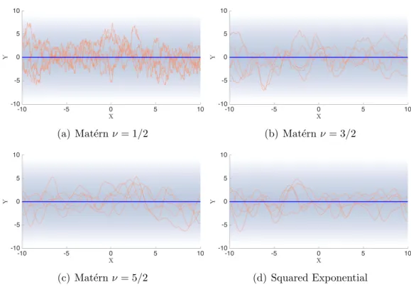
Despite the GP being a non-parametric approach to regression modelling, there are a number of user choices which must be made and hyperparameters which must be determined. These include the selection of the covariance function, which governs which functional family the process is drawn from. Although work has previously discussed kernel selection, for example [84–86], this has not been framed in an engineering context and discussion regarding the optimisation of hyperparameters is normally avoided. The author believes — and aims to show — that these are key parts of the modelling process which should be considered a matter of practice. This chapter discusses and demonstrates the effect and importance of these two issues. From Equations (2.11) and (2.12), it is clear that the kernel function plays a key role in the ability of the GP to make meaningful predictions. As discussed, the choice of kernel encodes the user’s prior belief as to which functional family the data is drawn from, which includes belief about smoothness, periodicity, linearity, and other properties. For example, if the kernel function is chosen to be linear, the solution for Bayesian linear regression is recovered exactly, this is further explored in Section 2.3.
In addition to this, each kernel function is controlled by one or more hyperparameters which alter the behaviour of that kernel. It is necessary to determine the “correct” hyperparameters for any given model as these control key behaviours of the function, such as the frequency of repeating behaviour, in a periodic kernel, or the total magnitude of the function. This is the commonly adopted view of the hyperparameter estimation problem as a parameter estimation. The usual manner in which this is approached is as a Type-II maximum likelihood estimate, which is to maximise the model evidence p(y|X). A Bayesian approach to this problem is possible (and arguably preferable) through the application of hyperpriors, as will be discussed. Consider the typical kernel which is used when introducing GP models [74], the squared exponential (SE) kernel — also called Gaussian or exponentiated quadratic — which has the following form.
k(x,x0) = σ2fexp −kx−x 0k2 2 2`2 (2.15)
where`is the length scale of the process which governs the smoothness of the function. Since choosing the kernel is equivalent to making some prior assumptions about the type of function you are trying to model, the choice of an SE kernel encodes the belief that the function being modelled is smooth, infinitely differentiable, and nonlinear. Following the choice of kernel, the specific function being modelled is conditioned on two things, foremost the observed training data in a Bayesian manner, but also the hyperparameters of the kernel.
As an example, the SE kernel is defined by two hyperparameters, the signal variance,
σf2, and the length scale, `. The signal variance affects the total scaling of the kernel, a larger signal variance is associated with signals which have higher variance, in fact this hyperparameter is actually the prior variance over the signal. That is, if no data are available for training, what the expected variance of the output would be around the mean of the process (usually zero).
Interpreting the length scale is slightly more difficult. In the case of the SE kernel it moderates the region of influence of each data point, or how close one data point needs to be to another in order to have an effect on the output. In Figure 2.5, the covariance k(x,x0) is plotted against the input distance for different length scales. It can be seen that by increasing the length scale parameter, points which are further away in the input space can still influence the outputs. This has the effect of
28 2.2. LEARNING GAUSSIAN PROCESSES FOR SHM
0
2
4
6
8
10
0
0.2
0.4
0.6
0.8
1
Figure 2.5: Increasing the length scale in the squared exponential kernel is shown to increase the region of influence. There is a higher covariance k(x,x0) at greater input distance |x−x0|as the length scale increases
‘smoothing out’ the function and removing short scale variations.
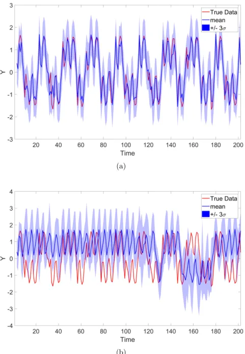
Practically, this means that, if the lengthscale parameter is large, the function being modelled will be smoother and if the lengthscale is shorter, the process will be less smooth. This is demonstrated in Figure 2.6 where the function is defined by a GP where three different length scales are used but other hyperparameters are fixed. If the length scales are set too long, as in the top figure, then all the observed data is considered as noise and the GP will not make meaningful predictions as well as being overconfident when predicting far from observed data. If the length scale is set too short, as in the bottom figure, the prediction of the GP quickly returns to the mean of the process, in this case zero. The means that there is only a very limited range of values for which the GP will return a meaningful prediction. The question remains as to how to specify the ‘optimal’ set of hyperparameters.
Before discussing this selection of hyperparameters, it is worthwhile considering one more commonly used technique when specifying the kernel function. In cases where there exists more than one dimension in the input data, it can be useful to place
Figure 2.6: Predictions from GPs with varying length scales, training points shown in red and test points in grey, the prediction both in the mean, solid blue line, and the 3σ confidence intervals shaded in blue. It can be seen that changing the lengthscale alters the smoothness of the process.
separate lengthscales over each of these dimensions. This is usually referred to as an Automatic Relevance Determination (ARD) kernel where the single hyperparameter,
`, is replaced with a matrix, Λ, which is a diagonal matrix with the individual length scales along the diagonal. This allows different dimensions of the input to operate over different scales and also provides information as to which of the input dimensions are contributing to which behaviours in the output. It is important also to consider that the noise variance of the process is rarely knowna priori, meaning it is normally included as an additional hyperparameter.
In the context of emulators — where a computationally cheaper model is used to replace an expensive simulator for calibration or Monte-Carlo analysis — Andrianakis and Challenor [87] discuss the role of the “nugget” — which replaces the noise term in a noise free emulator setting. For emulators (at least of deterministic simulators) it is assumed that the output of the simulator can be modelled as a noise free function — Gaussian Processes are one powerful approach to building these emulators. Within the Gaussian Process, the noise variance helps to stabilise the model numerically which poses a problem in the noise free emulator setting. For this reason a “nugget” term is usually set by the modeller. The paper of Andrianakis and Challenor [87] discusses how there can be two “modes” of solution (not related to dynamic modes) corresponding to either a Type-I or Type-II solution. The Type-I solution occurs
30 2.2. LEARNING GAUSSIAN PROCESSES FOR SHM
in the case of very low noise solutions to the GP (or when the nugget is set to be very small) in this mode the latent function passes through all the observed training points and leads to short lengthscales. This behaviour can be associated with “fitting the noise” in a model where the true underlying function is not captured in favour of attempting to explain all of the observed variability. This can be viewed as analogous to overfitting in a parametric model if the noise in the function is not actually very low. The alternative, Type-II solutions correspond to higher noise solutions where more of the function behaviour is explained as noise (or by the nugget in the emulator). In measured data, this can be a more realistic behaviour. However, the extreme of this is that the GP fails to model the underlying function instead modelling the functional behaviour as noise. This is a less dangerous misspecification of the model than fitting a Type-I solution when it is inappropriate. However, these solutions will lead to greater predictive uncertainty which can be just as costly if the models are used as part of a Risk & Reliability based inspection system through an increased need to inspect.
The question remains, how does a user ensure appropriate behaviour, for the available dataset. In this work, the author proposes two things, the first being to consider if a fully Bayesian solution is viable since understanding the full posterior over the hyperparameters will allow more informed decision making. Usually this is not possible practically. In that case, the second approach must be taken; to find an ‘optimal’ set of hyperparameters via optimisation. It is important to ensure robustness in the solution in one of a number of ways:
1. Begin gradient descent optimisation close to hyperparameters where there is good prior belief, i.e. low or high noise assumptions
2. If this cannot be done run multiple restarts of gradient descents to minimise the risk of local minima
3. Consider the use of a “global” optimisation scheme — such as the Quantum Particle Swarm Optimisation (QPSO)
4. Consider modifying the cost function of the optimisation
Within the machine learning community, most focus has been on achieving computa-tionally feasible solutions to the Bayesian estimation problem for the hyperparameter