OpenBU http://open.bu.edu
Theses & Dissertations Boston University Theses & Dissertations
2018
Learning to predict under a budget
https://hdl.handle.net/2144/30726
COLLEGE OF ENGINEERING
Dissertation
LEARNING TO PREDICT UNDER A BUDGET
by
FENG NAN
B.S., National University of Singapore, 2008
M.S., Massachusetts Institute of Technology, 2009
Submitted in partial fulllment of the
requirements for the degree of
Doctor of Philosophy
2018
FENG NAN
First Reader
Venkatesh Saligrama, PhD
Professor of Electrical and Computer Engineering Professor of Systems Engineering
Professor of Computer Science
Second Reader
David A. Castañón, PhD
Professor of Electrical and Computer Engineering Professor of Systems Engineering
Third Reader
Lorenzo Orecchia, PhD
Assistant Professor of Computer Science
Fourth Reader
Alexander Olshevsky, PhD
Assistant Professor of Electrical and Computer Engineering Assistant Professor of Systems Engineering
I have been fortunate to receive much support for the work of this thesis.
First, I am happy to give thanks to God and the Lord Jesus Christ for His love. He opened the door for me to pursue doctorate study and has carried me through.
I would also like to thank my advisor Professor Venkatesh Saligrama for his guid-ance and encouragement. The breath and depth of his intellect will continue to be my aspiration. In addition, I have learned what doing good research is about from seeing him at work. It is about being optimistic and enjoying the process even when the goal seems far; it is also about never giving up an idea without knowing why it does not work.
I also had the privilege of working with Professor Yannis Paschalidis, who kindly mentored me for the rst year at BU and introduced me to topics in computational biology. I would also like to acknowledge Professor David Castañón and Professor Lorenzo Orecchia for their availability to share their insights with me on optimization. I also thank Professor Alexander Olshevsky for agreeing to be on my thesis committee. I must also thank my colleagues and friends in BU for their numerous help and encouragement. They made my doctorate study a lot more enjoyable.
Last but not least, I would like to thank my family, especially my wife Yanping. She gave up much to support me through my study and gave birth to our two beautiful girls. Her sacrice and support are indispensable to my success. I also thank our parents for their seless love and unconditioned support.
FENG NAN
Boston University, College of Engineering, 2018
Major Professor: Venkatesh Saligrama, PhD
Professor of Electrical and Computer Engineering
Professor of Systems Engineering
Professor of Computer Science
ABSTRACT
Prediction-time budgets in machine learning applications can arise due to mon-etary or computational costs associated with acquiring information; they also arise due to latency and power consumption costs in evaluating increasingly more complex models. The goal in such budgeted prediction problems is to learn decision systems that maintain high prediction accuracy while meeting average cost constraints during prediction-time.
In this thesis, I will present several learning methods to better trade-o cost and error during prediction. The conceptual contribution of this thesis is to develop a new paradigm of bottom-up approaches instead of the traditional top-down approaches. A top-down approach attempts to build out the model by selectively adding the most cost-eective features to improve accuracy. It leads to fundamental combinatorial issues in multi-stage search over all feature subsets. In contrast, a bottom-up approach rst learns a highly accurate model and then prunes or adaptively approximates it to trade-o cost and error. We show that the bottom-up approach has several benets. To develop this theme, we rst propose two top-down methods and then two bottom-up methods. The rst top-down method uses margin information from
best feature in a greedy fashion or to stop and make prediction. The second top-down method is a variant of random forest (RF) algorithm. We grow decision trees with low acquisition cost and high strength based on greedy minimax cost-weighted impurity splits. Theoretically, we establish near-optimal acquisition cost guarantees for our algorithm.
The rst bottom-up method we propose is based on pruning RFs to optimize expected feature cost and accuracy. Given a RF as input, we pose pruning as a novel 0-1 integer program and show that it can be solved exactly via LP relaxation. We further develop a fast primal-dual algorithm that scales to large datasets. The second bottom-up method is adaptive approximation, which signicantly generalizes the RF pruning to accommodate more models and other types of costs besides feature acquisition cost. We rst train a high-accuracy, high-cost model. We then jointly learn a low-cost gating function together with a low-cost prediction model to adaptively approximate the high-cost model. The gating function identies the regions of the input space where the low-cost model suces for making highly accurate predictions. We demonstrate empirical performance of these methods and compare them to the state-of-the-arts. Finally, we study adaptive approximation in the on-line setting to obtain regret guarantees and discuss future work.
1 Introduction 1
1.1 Resource-constrained Machine Learning: Motivation . . . 1
1.2 Problem Denition . . . 3
1.2.1 Feature Acquisition Cost . . . 4
1.2.2 Computational Cost . . . 5 1.2.3 Communication/Latency Cost . . . 5 1.3 Challenges . . . 5 1.4 Contribution . . . 7 1.5 Related Work . . . 8 1.5.1 Non-adaptive methods . . . 9
1.5.2 Fixed feature acquisition . . . 9
1.5.3 Myopic feature acquisition . . . 10
1.5.4 Non-myopic feature acquisition . . . 11
1.5.5 Other methods . . . 12
1.6 Organization . . . 13
2 Margin-based Nearest Neighbor Approach 15 2.1 Related Work . . . 16
2.2 Problem Setup . . . 16
2.3 Algorithm . . . 19
2.4 Experiments . . . 21
3.1 Related Work . . . 26
3.2 Problem Setup . . . 27
3.3 Algorithm . . . 28
3.4 Bounding the Cost of Each Tree . . . 30
3.4.1 Admissible Impurity Functions . . . 35
3.4.2 Discussions . . . 38
3.5 Experiments . . . 40
4 Pruning Random Forests 49 4.1 Related Work . . . 51
4.2 Problem Setup . . . 52
4.2.1 Pruning with Costs . . . 53
4.3 Theoretical Analysis . . . 56
4.3.1 A Naive Pruning Formulation . . . 59
4.4 Algorithm . . . 61
4.5 Experiments . . . 65
4.5.1 Baseline Comparison . . . 65
4.5.2 Additional Experiments . . . 70
4.5.3 Discussion and Conclusion . . . 73
5 Adaptive Approximation 75 5.1 Related Work . . . 78
5.2 Problem Setup . . . 79
5.3 Algorithms . . . 84
5.4 Experiments . . . 87
6 On-line Adaptive Approximation 95 6.1 Problem Setup . . . 95
6.3 Lower Bound . . . 100
7 Future Work 103 7.1 Distributed Prediction . . . 103
7.1.1 Adaptive Sparse Regression . . . 104
7.1.2 Local Convexity - Hessian Computation . . . 105
7.1.3 Optimization . . . 106
7.1.4 Theorems to be proved . . . 107
7.1.5 Algorithms . . . 108
7.1.6 Experiments . . . 109
7.2 Extending the Regret Lower Bound . . . 112
7.2.1 Non-uniform sampling of patterns . . . 114
8 Conclusions 120 A Appendix 122 A.1 Adapt-Lstsq for Chapter 5 . . . 122
A.2 Experimental Details for Chapter 5 . . . 124
A.2.1 Synthetic-1 Experiment . . . 124
A.2.2 Synthetic-2 Experiment: . . . 124
A.2.3 Letters Dataset (Dheeru and Karra Taniskidou, 2017) . . . 124
A.2.4 MiniBooNE Particle Identication and Forest Covertype Datasets (Dheeru and Karra Taniskidou, 2017): . . . 126
A.2.5 Yahoo! Learning to Rank(Chapelle et al., 2011): . . . 127
A.2.6 CIFAR10 (Krizhevsky, 2009): . . . 128
References 129
Curriculum Vitae 135
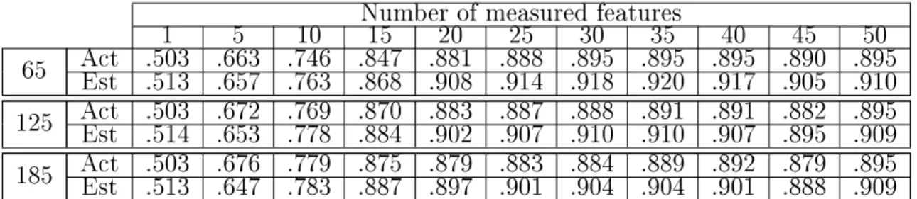
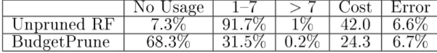
2.1 The actual and estimated probabilities of correct classication for neigh-borhood sizes 65, 125 and 185. . . 22 4.1 Typical feature usage in a 40 tree RF before and after pruning (our
algorithm) on the MiniBooNE dataset. Columns 2-4 list percentage of test examples that do not use the feature, use it 1 to 7 times, and use it greater than 7 times, respectively. Before pruning, 91% examples use the feature only a few (1 to 7) times, paying a signicant cost for its acquisition; after pruning, 68% of the total examples no longer use this feature, reducing cost with minimal error increase. Column 5 is the average feature cost (the average number of unique features used by test examples). Column 6 is the test error of RFs. Overall, pruning dramatically reduces average feature cost while maintaining the same error level. . . 50 5.1 Dataset Statistics . . . 90
2·1 An example of cost sensitive learning. Given 8 training points, each is binary with 3 features: x(1) = x(2) = (1,−1,−1), x(3) = x(4) = (−1,1,1), x(5) = (−1,1,−1), x(6) = x(7) = x(8) = (1,1,1), with labels
y(1), . . . , y(4) =−1, y(5), . . . , y(8) = 1. They are linearly separable with
optimal SVM solutiony=w′∗x+b = (0.9995,1.4998,−0.5002)x−0.9997 20
2·2 Experiment result of classication accuracy vs number of features mea-sured on Letters, LandSat MiniBooNE datasets. FMCC is consistent across all datasets while the VoC does not perform well on the Mini-BooNE dataset. . . 24 3·1 A synthetic example to show max-cost of GreedyTree can be smoothed
to approach the expected-cost. The left and right gures above show the classier outcomes of featuret1 and t2, respectively. . . 39
3·2 The error-cost trade-o plot of the subroutine GreedyTree using threshold-Pairs on the synthetic example. 0.39% error can be achieved
using only a depth-2 tree but it takes a depth-10 tree to achieve zero error. . . 40 3·3 Comparison of BudgetRF against ASTC (Kusner et al., 2014) and
CSTC (Xu et al., 2013) on 4 real world datasets. BudgetRF has a clear advantage over these state-of-the-art methods as it achieves high accuracy/low error using less feature costs. . . 42
function in (3.13) for l = 2,3,4,5 and the threshold-Pairs impurity
function. Note that for both House Votes and WBCD, the depth0tree
is not included as the error decreases dramatically using a single test. In many cases, the threshold-Pairs impurity function outperforms the Powers impurity functions for trees with smaller max-costs, whereas the Powers impurity function outperforms the threshold-Pairs function for larger max-costs. . . 48 4·1 An ensemble of two decision trees with node numbers and associated
feature in subscripts . . . 58 4·2 Turning pruning to equivalent shortest path problems. . . 64 4·3 Comparison of BudgetPrune against CCP, BudgetRF with early
stopping, GreedyPrune and GreedyMiser on 4 real world datasets. BudgetPrune (red) outperforms competing state-of-art methods. GreedyMiser dominates ASTC (Kusner et al., 2014), CSTC (Xu et al., 2013) and DAG (Wang et al., 2015) signicantly on all datasets. We omit them in the plots to clearly depict the dierences between competing methods. . . 66 4·4 Comparing BudgetPrune and CCP with uniform and non-uniform
feature cost on MiniBooNE dataset. BudgetPrune is robust when the feature cost is non-uniform. . . 71 4·5 Comparisons of various pruning methods based on entropy and Pairs
splitting criteria on MiniBooNE and Forest datasets . . . 72
k=120 on Scene15 dataset. The initial RF has higher accuracy and higher cost for k=20. GreedyPrune performs very well in k=20 but very poorly in k=120. . . 72 5·1 Left: single stage schematic of our approach. We learn low-cost
gat-ing g and a LPC model to adaptively approximate a HPC model.
Right: Key insight for adaptive approximation. x-axis represents fea-ture space; y-axis represents conditional probability of correct predic-tion; LPC can match HPC's prediction in the input region correspond-ing to the right of the gatcorrespond-ing threshold but performs poorly otherwise. Our goal is to learn a low-cost gating function that attempts to send examples on the right to LPC and the left to HPC. . . 76 5·2 Synthetic-1 experiment without feature cost. (a): input data. (d):
decision contour of RBF-SVM as f0. (b) and (c): decision boundaries
of linear g and f1 at initialization and after 10 iterations of
Adapt-Lin. (e) and (f): decision boundaries of boosted tree g and f1 at
initialization and after 10 iterations of Adapt-Gbrt. Examples in the beige areas are sent to f0 by the g. . . 88
5·3 A 2-D synthetic example for adaptive feature acquisition. On the left: data distributed in four clusters. The two features correspond to x and y coordinates, respectively. On the right: accuracy-cost trade-o curves. Our algtrade-orithm can rectrade-over the trade-optimal adaptive system whereas a L1-based approach cannot. . . 89
Prune on four benchmark datasets. RF is used asf0for Adapt-Gbrt
in (a-c) while an RBF-SVM is used asf0 in (d). Adapt-Gbrt achieves
better accuracy-cost tradeo than other methods. The gap is signi-cant in (b) (c) and (d). Note the accuracy of GreedyMiser in (b) never exceeds 0.86 and its precision in (c) slowly rises to 0.138 at cost of 658. We limit the cost range for a clearer comparison. . . 91 5·5 Compare the L1 baseline approach, Adapt-Lin and Adapt-Gbrt
based on RBF-SVM and RF asf0's on the Letters dataset. . . 93
6·1 Feedback graph for four experts. ξ1andξ2request for label and receives
full feedback; ξ3 and ξ4 classify using h and receives no feedback. . . . 96
7·1 A distributed mixture of expert model for . . . 104 7·2 Sigmoid parameter is the constant multiplier inside the exponential of
the sigmoid function; noise is the noise level; ss is the step size . . . . 119
DAG . . . Directed Acyclic Graph
GBRT . . . Gradient Boosted Regression Tree RF . . . Random Forest
ℜK . . . the K-dimensional Euclidean space
Chapter 1
Introduction
1.1 Resource-constrained Machine Learning: Motivation
Machine learning plays an increasingly important role in many scientic and engi-neering problems. It includes problems such as classication, regression, ranking, clustering and so on. Much of machine learning research has focused on improving accuracy. But more recently, as the scale and complexity of machine learning appli-cations grow, costs in both training and test time have gained importance. To limit scope, we consider exclusively supervised learning in this thesis. Training time thus typically involves the cost of collecting labeled data and the computational cost of processing the collected data to learn the model. In many applications such as health care, labeled data is scarce and expensive. The area of active learning (Settles, 2009) is devoted to eciently using fewer labeled examples to train models. Once a model is trained, it is used for prediction of new examples. Prediction-time costs can arise due to monetary costs associated with acquiring information or computation time (or delay) involved in extracting features and running the algorithm; they can also arise in mobile computing due to limited memory, battery and communication.
In many machine learning applications training can be carried out o-line, sep-arate from the production system. On the other hand, prediction typically occurs in production and is subject to more stringent budget constraints. Therefore, this thesis focuses primarily on reducing costs incurred during prediction or test time. Only toward the end (Chapter 6) we will discuss an on-line learning scenario where
we bring together training and test time costs. Consider the following applications as motivation for prediction time budget constraints.
• Automated medical diagnosis: This is a classication task. During training, an algorithm is given medical records of diagnosed patients as input features and the diagnosis as labels. The goal is to learn a model to automatically diagnose new patients based on the outcome of their medical test results. Some of these medical tests are simple and inexpensive such as blood pressures, vitals. Others are more expensive and could potentially be harmful to the human body such as X-ray, MRI. The prediction time cost consists of the monetary cost of each medical test as well as its associated risk. When a new patient is presented to the system, it is thus undesirable to require him or her to undertake all possible medical tests and then make a prediction. Instead, we aim to learn a system that recommends only the necessary medical tests to reduce cost while maintaining high diagnosis accuracy.
• Document ranking: (Chapelle et al., 2011) This is a ranking task. During training, an algorithm is given a set of queries as well as a set of documents associated with each query ranked according to the relevance to the query. The goal is to learn a model so that given a new query and a set of documents, it can rank the documents according to the relevance to the query. To achieve this, features of each query-document pair must be extracted. Some features are cheap to extract, such as key word search; other features are computation-ally more expensive, such as textual similarity and proximity measures. Each of these features require CPU time to extract, yet the ranking has to be done in milliseconds to be displayed to the user. This precludes extraction of com-putationally expensive features for all query-document pairs. We aim to learn a system that extracts the expensive features only if it is necessary to reduce
cost while maintaining high ranking accuracy.
• Deep neural networks (DNNs): DNNs have been successfully applied in many application including visual object recognition, speech recognition and machine translation. They achieve the state of the art accuracy yet require considerable computational budget during prediction due to their increasing complexity. For example, the Resnet152 (He et al., 2016) architecture with 152 layers has 4.4% accuracy gain in top-5 performance over GoogLeNet (Szegedy et al., ) on the large-scale ImageNet dataset (Russakovsky et al., 2015) but is 14X slower at test-time(Bolukbasi et al., 2017). We aim to learn systems that can reduce the computational cost while maintaining high accuracy.
• Mobile computing, Internet of Things (IoT): Smart devices include phones, watches, cameras and sensors (known as edge devices) have been widely used to gather and process information for tasks such as activity recognition and surveil-lance. Such devices typically have limited battery, memory and computational power. Machine learning models that run on such devices are constrained by these physical limitations. For real-time applications, there is also a communi-cation cost in terms of latency whenever the edge devices communicate with the server(cloud). We aim to develop machine learning systems that are suitable to be deployed on such edge devices and use small budget to achieve high accuracy.
1.2 Problem Denition
In this section, we introduce some basic notations and present the general problem of learning with prediction-time costs similar to the formulation in (Trapeznikov and Saligrama, 2013; Wang et al., 2014b). We focus on the supervised setting where we assume fully annotated datasets are available for training. We seek to learn deci-sion systems that maintain high-accuracy while meeting average resource constraints
during prediction-time.
Suppose an example-label pair (x, y)is drawn from distributionP. The goal is to
learn a prediction function f from a family of functions F that minimizes expected
prediction error subject to a budget constraint:
min
f∈F E(x,y)∼P[err(y, f(x))], s.t. Ex∼Px[C(f, x)]≤B, (1.1)
where err(y,yˆ)is the error function; C(f, x) is the cost of evaluating the functionf
on example x and B is a user specied budget constraint.
In practice, we are not given the distribution but instead are given a set of train-ing data (x(1), y(1)), . . . ,(x(n), y(n)) drawn i.i.d. from distribution P. We can then
minimize an empirical approximation of the expected error function:
min f∈F 1 n n ∑ i=1 L(y(i), f(x(i))), s.t. 1 n n ∑ i=1 C(f, x(i))≤B, (1.2)
where L(y,yˆ) is a loss function. Note our budget constraint is on prediction costs
averaged over the examples. This allows the exibility to spend the budget in an example-dependent manner.
The denition of C(f, x)is application specic as seen in the motivation examples
in Section 1.1. We shall focus on the feature acquisition cost in this thesis while addressing other types of costs such as computational and communication/latency costs as well.
1.2.1 Feature Acquisition Cost
Features (or covariates in statistics) are the numerical attributes associated with an input example. They provide information about the examples as a basis for prediction. There is often a cost associated with acquiring or extracting these feature values. Supposex∈ ℜK is the feature vector with an acquisition costc
of the features α= 1, . . . , K. 1
For a given example x, we assume that once it pays the cost to acquire a feature,
its value can be eciently cached; and subsequent use of the feature value does not incur additional cost. Thus, the cost of utilizing a particular prediction function, denoted by C(f, x), is computed as the sum of the acquisition cost of unique features
required by f forx.
1.2.2 Computational Cost
C(f, x) can also measure the amount of computation required to compute f(x). In
a decision tree f, for example, it is proportional to the number of internal nodes x
traverses. In a neural network, it is proportional to the number of layers and the number of connections between the layers.
1.2.3 Communication/Latency Cost
In mobile applications, predictionf(x)may involve communication between the edge
device and the server (cloud). C(f, x) can capture such costs in terms of
communi-cation/latency cost.
1.3 Challenges
The problem of learning to prediction under a budget might appear well-studied as formulated in Eq.(1.2), which consists of an empirical loss minimization subject to a constraint. Indeed, the sparse learning or feature selection problem is an instance of learning to predict under a budget. Consider each feature element carries a unit acquisition cost and F is the space of linear regressors. Each f ∈ F can be
parame-1Note that our algorithms can be adapted to handle group-structured features where several
elements inxmay be associated with one feature acquisition cost. In other words, several elements
in thexvector can be obtained together by paying the acquisition cost for one feature. We avoid it
terized by w ∈ ℜK. The cost C(f, x) is equal to the number of non-zero elements in
w: C(f, x) =∥w∥0. The budget constraint on the prediction-time feature acquisition
cost thus reduces to a sparsity constraint on w. The sparse linear regression problem
is min w∈ℜK 1 n n ∑ i=1 ( y(i)−wTx(i))2, s.t. ∥w∥0 ≤B. (1.3)
Algorithms including LASSO (Tibshirani, 1996) and other subset selection methods have been well established (Miller, 2002). Yet we highlight that the goal of traditional sparse learning or feature selection is to identify a subset of the features to be used for all the examples. The assumption is that there exists a common subset of features that are useful for predicting all examples. But in practice, dierent examples may benet from dierent subsets of features. Consider the medical diagnosis example, it makes sense to recommend dierent subsets of medical tests for dierent patients, depending on their individual conditions. In other words, the decision functions that we seek to learn are more general, able to adapt to dierent input examples.
The key idea in our budgeted prediction framework is to recognize that in many machine learning tasks not all input examples are created equal. There are easy examples that can be predicted at low cost (e.g. using a few low cost features or going through a small number of layers in a neural network). Only the dicult examples require more cost (e.g. using more features or going through many layers in a neural network). Since the budget constraint is on the average prediction cost over the examples, we can achieve high prediction accuracy by allocating less budget on the easy examples and more budget on the dicult ones.
In some sense, the family of decision functions F in Eq. (1.2) that we optimize over is a family of adaptive decision rules, or decision policies, rather than static models such as a linear predictor. We highlight several challenges this entails.
• Distinguish easy V.s. dicult examples: Given a training dataset, it is not clear how to partition the examples into easy V.s. dicult ones. The partition function itself is a classier that needs to be learned. Furthermore, how the dataset is partitioned impacts the data distribution for the downstream prediction models. In other words, the partition function should be learned jointly with a cheap prediction model that handles the easy examples as well as an expensive prediction model that handles the dicult ones. This inter-dependency translates to products of indicator functions in the optimization objective and leads to non-convexity.
• Combinatorial state space: With feature acquisition costs, the adaptive decision rule can be represented by a Directed Acyclic Graph (DAG) (Wang et al., 2015). The internal nodes correspond to feature subsets and decision functions at each node choose whether to acquire a new feature or predict using the already acquired features. The edges correspond to acquiring new features, transitioning from one feature subset to another. The number of states, or feature subsets, is 2K, where K is the number of features. Learning decision
functions for each state becomes intractable when the number of features is large.
1.4 Contribution
We develop several novel algorithmic approaches to the learning under prediction budget problem, improving the state of the art performance with each method. More importantly, through these methods, we develop a new bottom-up paradigm for the learning under prediction budget problem. Here we give a summary of the contribu-tions made in this thesis.
margins in classication.
• We propose to learn the adaptive decision rule as random forests. We propose a family of impurity measures and a splitting criteria so that the decision trees we grow are guaranteed to have near-optimal feature acquisition costs.
• Given any random forest, we propose to prune it to optimize expected feature cost & accuracy. We pose pruning RFs as a novel 0-1 integer program and estab-lish total unimodularity of the constraint set to prove that the corresponding LP relaxation solves the original integer program. We further exploit connections to combinatorial optimization and develop an ecient primal-dual algorithm that scales to large problems. This bottom-up pruning approach circumvents the need for combinatorial search faced by the top-down approaches.
• We develop an adaptive approximation framework as a general bottom-up ap-proach. The framework incorporates general machine learning models such as RF, boosting, SVM and neural networks. It also accounts for various types of costs such as feature acquisition, computational and communication/latency costs.
• We propose an on-line learning framework for the adaptive approximation and provide regret analysis.
1.5 Related Work
The problem of learning from full training data for prediction-time cost reduction (MacKay, 1992) has been extensively studied. We summarize related work according to the key properties in their approaches. We focus on the feature acquisition costs rst.
1.5.1 Non-adaptive methods
The non-adaptive methods reduce prediction-time cost by identifying a common sparse subset of features that are used by all examples. Some of these methods include subset selection (Miller, 2002) and L1 regularization (Tibshirani, 1996). The Greedy Miser (Xu et al., 2012) is a non-linear method in this category. It is an adaptation of gradient boosted regression trees in the setting of feature acquisition costs. The algorithm iteratively adds weak learners (low-depth regression trees) to the ensemble by trading o the goodness t to the current gradient and the additional feature cost introduced. The typical trees are limited to low-depth (4 or 5 levels) to avoid over-tting. As a result, we consider it a non-adaptive method because all the examples typically encounter the same set of features. Furthermore, the training algorithm does not consider feature usage at a per-example basis and it bears more similarity to a stepwise feature selection process. In contrast, the methods we propose in this thesis are adaptive in the sense that dierent examples can be routed dierently in the decision rule and incur dierent costs.
1.5.2 Fixed feature acquisition
Among the adaptive methods, some assume a feature acquisition graph is given a prior, which is xed by domain experts or enumerated in the case of just a few features. The task reduces to learning reject functions as well as end classiers in the case of detection cascades (Viola and Jones, 2001). (Trapeznikov and Saligrama, 2013) generalize detection cascades to classier cascades to handle balanced and/or multi-class scenarios. They solve a stage-wise empirical minimization problem and use cyclic optimization to iterate over the stages. (Wang et al., 2014b) extends the cascade to tree structures and formulated a convex surrogate that bounds the global empirical risk. (Wang et al., 2015) extend the tree structure to directed acyclic graphs
(DAGs) and trains decision functions for each node of the graph according to a child-to-parent order. In contrast to these methods based on xed feature acquisition graph, ours proposed in this thesis aim to learn such sequential feature acquisition graphs. 1.5.3 Myopic feature acquisition
Due to the combinatorial search space for sequential feature acquisition, many meth-ods resort to greedy/myopic strategies based on utility of acquiring each feature. (Ji and Carin, 2007) model the sequential decision process for feature acquisition and classication as a POMDP. But due to the diculty associated with a POMDP for-mulation such as high computational cost, the need to quantize features and the lack of mechanism to rule out repeated actions, the authors proposed a myopic approxima-tion. The utility of an action is evaluated by the dierence between its cost and the reduction in the Bayes risk, as computed from the probability model. On the other hand, (Kanani and Melville, 2008) propose to dene utility as dierence in unlabeled margin divided by feature acquisition cost. Without assuming probability model, they propose to estimate feature value distribution by discretizing the feature values and learning classiers based on available features to predict its distribution. (Gao and Koller, 2011) propose a locally weighted regression method during test time and assume a Gaussian model to myopically select features based on information gain of unknown features. The above methods tend to have high computational cost during prediction-time and require generative assumptions.
(Sheng and Ling, 2006) propose a sequential batch test algorithm to minimize total cost of acquiring features and misclassication. Used with decision trees, it selects features to split the internal nodes based on their utility values. This heuristic utility is dened as the dierence of the expected cost before and after acquiring the feature. In Chapter 3, we propose a dierent utility measure as well as splitting criteria that lead to near-optimal cost guarantee.
1.5.4 Non-myopic feature acquisition
In general, learning non-myopic feature acquisition rules is computationally intractable. However, under certain assumptions and for specialized settings, this is achievable. (Busa-Fekete et al., 2012) formulate the decision process as an MDP. The features they consider are ordered base learners obtained from AdaBoost. At each base learner, the actions to take are to Evaluate, Skip or Quit. The Quit action leads to a nal classication. The state is composed of the sum of evaluated weak learner outputs so far as well as the index of current base learner. By associating each Evaluate ac-tion with a cost, the MDP reward is to minimize the nal classicaac-tion loss plus the total cost. The formulation in (Busa-Fekete et al., 2012) is primarily based on the xed weak learner order, which helps reduce the action space. (Bilgic and Getoor, 2007) introduce a novel data structure called Value of Information Lattice (VOILA) to calculate value of information for subsets of features. VOILA is a directed graph where each node represents a unique subset of the features and each edge represents a subset relationship between its nodes. In order to reduce the exponential number of feature subsets, a Bayesian network over the features as well as the class variable is assumed given. (Karayev et al., 2012) formulates a problem of object recognition un-der time constraint as an MDP. The actions correspond to running dierent detectors or classiers. A state includes current estimates of the distribution of class presence, the history of actions taken together with the resulting observations, as well as the time costs so far and the time budget left. The state-action pair is featurized by con-catenating the prior distribution of the classes for the action, the distribution of the classes as well as the entropies for all classes conditioned on observations so far. The long term reward function Q is modeled as a inner product of the state-action pair
and a vector parameterizing the policy. A convenient property in the above problem is that the evaluation function is additive per action, as computed by the change in
average precision introduced by the action. (Zubek and Dietterich, 2002) also for-mulates the problem of classication with feature acquisition costs as an MDP. They use heuristic search algorithms to reduce the search space for the optimal policy. But this approach requires discretization of the feature values and is inecient when the state space is large.
Another line of methods aims to learn feature acquisition rules in a discriminative framework through empirical risk minimization. (Chen et al., 2012) aim to re-order a set of pre-training base learners to reduce prediction costs. It optimizes the param-eters of the stages in cycles. Multiple levels of relaxations are proposed to make the optimization objective continuous and dierentiable. Still, the proposed algorithm faces computational diculty as it needs to solve a non-convex optimization problem during each cycle.
(Xu et al., 2013) propose to learn a tree of classiers. The tree structure is a limited-depth balanced binary tree. Each path of the tree requires a dierent set of features so as to reduce test-time feature cost. Similar to (Chen et al., 2012), they propose to minimize the sum of losses at all internal nodes plus a weighted cost term. Several relaxations are used to make computation tractable. Cyclic optimization is used to learn the classier at each node while xing all other nodes. During test time, an example is routed at each internal node by a linear classier to determine the probability of going left or right and the branch is taken with respect to these probabilities. (Kusner et al., 2014) recognize that the method in (Xu et al., 2013) is hard to train and requires involved optimization hyperparameter tuning. They propose a simpler training procedure based on greedy selection.
1.5.5 Other methods
Besides feature acquisition costs, many researchers have considered reducing com-putational costs as well as memory usage during prediction-time. The distillation
framework (Hinton et al., 2015; Lopez-Paz et al., 2016) aims to compress a complex teacher model into a smaller student model without losing much accuracy. (Kumar et al., 2017) propose a compact tree model called Bonsai that achieves high accuracy with small model size. (Gupta et al., 2017) propose PtotoNN as a compressed K-Nearest Neighbor algorithm. The main idea is to learn a small number of prototypes to represent the entire training set and jointly learn a projection matrix to reduce dimensionality as well. Reducing the prediction costs of deep neural networks has also been an area of recent interest (Bolukbasi et al., 2017; Lin et al., 2017).
1.6 Organization
The rest of this thesis is organized in the following manner:
Chapter 2 will describe a myopic algorithm for feature acquisition based on mar-gin and nearest neighbors. We will explain the intuitive advantage of this simple algorithm and also show numerical experiments.
Chapter 3 will describe a new decision tree growing algorithm that incorporates feature acquisition cost. Even though the algorithm is myopic, we will provide the-oretical guarantee to show that it achieves near-optimal cost. We then expand to ensembles of such decision trees and illustrate performance with numerical experi-ments.
Chapter 4 will describe a novel method to prune random forests to optimize feature acquisition costs and accuracy. We will provide detailed formulation and theoretical guarantee that the pruning optimization problem can be solved in polynomial time. We will further provide a specialized primal-dual algorithm that can scale to large datasets. Finally, we will evaluate the performance with numerical experiments.
Chapter 5 will motivate and describe a novel framework of adaptive approxi-mation of general models for prediction-time cost reduction. We will formulate an
optimization problem and point out the computational advantages compared to pre-vious approaches. This general framework is then specialized into linear and gradient boosted models. Again, we will evaluate the performance with numerical experiments. Chapter 6 will study the adaptive approximation problem in an on-line setting with limited feedback. We provide theoretical analysis of the regret.
Chapter 7 will discuss future directions. We will introduce the problem of dis-tributed prediction and explain our formulation. We will also show some preliminary experimental results. We will also consider extensions of the regret analysis of the on-line adaptive approximation problem.
Chapter 2
Margin-based Nearest Neighbor Approach
We introduce a novel algorithm to dynamically select features for every test instance until we reach a desired classication accuracy. We assume we have access to a training set with full features and corresponding class labels. For every test point, there is a cost associated with measuring or computing each feature. Our system acquires one feature at a time, adaptively deciding which feature to request next or when to stop and classify. We learn such a policy by utilizing training examples within a neighborhood of a test point. The key challenge in learning such a decision system is to correctly determine the neighborhood. After acquiring a partial set of features, we can not infer the true distance from a test point to training points in the full feature space. In other words, the nearest neighbor based on partial feature measurement may not be a true neighbor in the full feature space. We call this diculty partial neighborhood confusion. Algorithms that try to learn the label of a test point based on the labels of training points in the partial neighborhood tend to perform poorly due to this diculty.
In contrast, to make our approach more robust to such partial neighborhood con-fusion, we incorporate classication margins in our system. In binary classication, a margin of an example is typically an output of a decision functions times the label (+1/−1) of an example. Margins are widely used as a measure of classication
con-dence. A large positive margin indicates high condence, while a negative margin indicates an incorrect decision. Maximizing margins has led to many powerful tools
in machine learning such as SVM, boosting, etc ((Cortes and Vapnik, 1995)). We use margins to estimate the probability of correct classication and sequentially maxi-mize this probability at each stage of the decision making process. Since the label of a test point is unknown, its margin cannot be computed directly. To overcome this problem, our algorithm learns the unknown test margin from the training data in the partial neighborhood of this test point. Recall that feature values and labels are known for the training data, hence margins are also fully known. Since our algo-rithm learns margin information instead of class label from nearest neighbors based on partial feature measurement, we are more robust to the partial neighborhood con-fusion problem. Intuitively, points far from each other in the full feature space are unlikely to share the same label but may produce the same sign margins on the same feature. We will illustrate this point further through an example in Section 2.3 and Experiments in Section 2.4.
The work presented in this chapter is published in (Nan et al., 2014).
2.1 Related Work
The method we propose in this chapter involves myopic feature acquisition as dis-cussed in Section 1.5. Dierent from (Ji and Carin, 2007; Gao and Koller, 2011), we do not assume specic probability distribution. Dierent from (Kanani and Melville, 2008), we use labeled margin of nearest neighbors rather than unlabeled margin.
2.2 Problem Setup
Given the training set of N data points and corresponding labels (x(l), y(l)), l = 1, . . . , n, each point hasdfeaturesx(l) ∈ ℜd, and we assume all features are known for
training. Given an unknown test point, a featurej can be measured or acquired for a
on the entire training set. Note we omit the oset term in our discussion because it can be considered as an additional (constant) feature of the data point.
Remark: We assume a linear classier is used for the entire data set. This is not as restrictive as it may appear. In fact, kernel SVM is linear in the transformed feature space and Boosting (Freund and Schapire, 1997) is linear once we consider weak learners as transformed features. We will show in our experiment that our algorithm works with both SVM and Boosting.
In the rest of this section, we explain our dynamic feature selection approach for a new test point,x. Let O be the index set of measured features and O be the index
set of the remaining features. We use wO to denote the elements of windexed by O.
For ease of notation we use i to denote the index of the next potential feature to be
measured. InitiallyO =∅. We can choose the most discriminative feature as the rst
feature. LetxO denote the measurement values obtained about the test point and we
set the unmeasured feature values to be 01, x
O = 0. If a classication is needed with
the current measurements we can simply compute
y=wOTxO, (2.1)
and decide based on its sign.
Given any measured feature setO, it is not clear howwTOxOrelateswTx(a decision
when all features are measured). However, assume we choose the features in O to produce positive margins on the neighboring training points. In this scenario, these features will most likely also produce positive margins on the test point and result in accurate classication based on (2.1). To be more concrete, we dene a partial neighborhood N(O) of the test point as the index set of those training points that
are close toxO on the index setO. We deneN(O)to contain theKnearest neighbors
1Note that this is a missing feature classier. While there has been some work (see (Maaten
(with respect to Euclidean distance) of xO in the training set, where K is a positive
natural number.2
Next, dene the partial margin of the kth training point in the neighbood N(O)
based on the current measurement feature set O as
ηkO =y(k)(wTOxO(k)), k∈N(O). (2.2)
If ηOk is positive then (2.1) will give correct classication based on the measured
feature set O. Similarly, dene the one-step-ahead partial margin of thekth training
point in the neighbood N(O) based on the current measurement feature set O and
feature i as
ηi,kO =y(k)(wOTx(Ok)+wix (k)
i ), k ∈N(O), i∈ O. (2.3)
To estimate classication accuracy, we dene the partial probability of correct clas-sication of the test point based on current measurement feature set O as the ratio of the number of correct classications to the total number of training points within the neighborhood:
pO = #{k :η O
k >0}
|N(O)| . (2.4)
Similarly we dene the one-step-ahead partial probability of correct classication of the test point based on current measurement feature set O and feature ias
pOi = #{k :η O
i,k >0}
|N(O)| . (2.5)
At each step, we can decide to measure the next feature or to stop based on the accuracy estimate pO. And pOi provides an estimate of how much accuracy we can
get by measuring ias the next feature. We can thus choose the i that gives the best
accuracy-cost trade-o.
2While there are many ways to dene a neighborhood (i.e. based on thresholding a distance
2.3 Algorithm
We present our algorithm in Algorithm 1.
Algorithm 1 Fast Margin-based Cost-sensitive Classication (FMCC) 1: Train classier y=wTx on the entire training data
2: Fix accuracy-cost tradeo parameter α
3: Given a test pointx:
4: Measure feature i
5: for t = 1→d do ◃Iterate through the total number of features
6: if pO >threshold then
7: Stop, make classication 8: else
9: Compute neighborhood N(O)
10: for i∈ O do
11: Update partial marginsηi,kO for k ∈N(O) according to (2.3)
12: Compute pOi according to (2.5)
13: Select featureimax =argmaxipOi −αci to measure next, O ←(O, imax).
14: Update partial marginsηOk for k ∈N(O) according to (2.2)
15: Compute pO according to (2.4)
Suppose there are 8 training data points as shown in Figure 2·1. The class labels are indicated in red disks (label −1) and black triangles (label 1), with the weight
(number of repeated training examples) shown besides them. For each training point, we also display the coordinates. By inspection, to locate an unknown test point (assuming it follows the distribution of the training data), the optimal strategy would be to measure x2, then x1 and lastly x3. We show that our algorithm indeed follows
x1
x2
x3
(1,-1,-1)
(-1,1,-1)
(1,1,1)
(-1,1,1)
2
2
3
1
Figure 2·1: An example of cost sensitive learning. Given 8 training points, each is binary with 3 features: x(1) =x(2) = (1,−1,−1), x(3) =
x(4) = (−1,1,1), x(5) = (−1,1,−1), x(6) = x(7) = x(8) = (1,1,1), with
labelsy(1), . . . , y(4) =−1, y(5), . . . , y(8) = 1. They are linearly separable
with optimal SVM solutiony=w′∗x+b= (0.9995,1.4998,−0.5002)x−
0.9997
Suppose all the features carry the same measurement cost. And the partial neigh-borhood is dened to be those training points having exactly the same feature values as the test point onxO. We apply our algorithm sequentially as follows. Step 1.
Mea-suringx1, x2, x3 will give2+2 = 4,2+1+3 = 6,2+2 = 4correct classications based
on (2.1), respectively. So measuring x2 will result in higher accuracy. Step 2.
Sup-pose x2 has been measured and it's equal to -1, there are 2 points in N(O) = {1,2}.
Compute η1O = ηO2 > 0 using (2.2). So the estimated accuracy pO = 1. Stop and
classify, giving the correct classication. Suppose x2 is measured to be 1, there are 6
points inN(O) = {3,4,5,6,7,8}. As we contemplate on measuring x1 next, compute
ηO1,3 =η1O,4 >0, ηO1,5 <0, ηO1,6 =η1O,7 =η1O,8 >0using (2.3). Therefore we obtainpO1 = 56
in higher accuracy, which agrees with the optimal strategy.
Analysis: When the full set of features are measured, pO in (2.4) is unbiased
estimator of the correct classication probability. The training points in the neigh-borhood N(O) obey the probability distribution of the training points. And (2.4)
is the sample mean of the actual classication accuracy according to (2.1). And we assume all data points are i.i.d hence we get the result. We can regard pO as a good
estimate of the probability of correct classication in the (nite) limit sense (when the number of measured features increases to the maximum). We can also show our algorithm has test time complexity that scales linearly in sample size. There are at most d iterations (the total number of features) and each iteration involves only
O(ndK) operations, where K is a constant neighborhood size. Thus, our algorithm
is well suited when the number of training examples are not too large or the test time computation budget is large. In contrast, the VoC algorithm requires solving a locally weighted least square problem at each iteration and the per iteration complexity is
O(n2d3), which is much higher.
2.4 Experiments
We evaluate our algorithm on three UCI data sets (Dheeru and Karra Taniskidou, 2017). To demonstrate the wide applicability of our algorithm, we base our algorithm on Boosting for the rst two data set and linear SVM for the third data set.
Performance Metric: A natural way to evaluate performance of budged learning is compare accuracy vs the number of features acquired. The objective is to achieve high classication accuracy while acquiring as few features as possible. We assume acquisition cost for all features is uniform.
Letter Recognition Data Set: This is a multi-class data set with the goal of distinguishing 26 capital letters in the English alphabet from a large number of
Number of measured features
1 5 10 15 20 25 30 35 40 45 50 65 Act .503 .663 .746 .847 .881 .888 .895 .895 .895 .890 .895Est .513 .657 .763 .868 .908 .914 .918 .920 .917 .905 .910 125 Act .503 .672 .769 .870 .883 .887 .888 .891 .891 .882 .895Est .514 .653 .778 .884 .902 .907 .910 .910 .907 .895 .909 185 Act .503 .676 .779 .875 .879 .883 .884 .889 .892 .879 .895Est .513 .647 .783 .887 .897 .901 .904 .904 .901 .888 .909
Table 2.1: The actual and estimated probabilities of correct classi-cation for neighborhood sizes 65, 125 and 185.
black-and-white rectangular pixel displays. Each data point consists of 16 features. We randomly draw 200 examples from each letter as training points and 100 examples as test points and assign the rst 13 letters to one class and the other 13 letters to the other class. Results are shown from 50 randomly drawn sets of data to prevent sampling bias. We train a boosted collection of 1000 stumps on the training set, where each stump thresholds a single feature. Evaluating the stumps for each feature yields a set of margins. For comparison, we implement the probabilistic model-based Value of Classier (VoC) algorithm (Gao and Koller, 2011), with the negative of classication loss as the reward function. We set λ = 0.5 in the locally weighted regression and
the bandwidth parameter β is set to be the median of the distances from the test
point to the training points at each step. We also compare to a random order scheme, where the next feature to measure is chosen at random and classication at each step is computed by (2.1). We see from Fig. 2·2 that our FMCC is close to VoC and outperforms the baseline. For small budgets (few observed features), VoC achieves higher accuracy than FMCC, however after measuring 6 features, FMCC outperforms VoC. This behavior is expected, as the estimated neighborhood of each example are unreliable when few features have been observed. Additionally, the FMCC algorithm has lower computational complexity than VoC; at each stage of feature acquisition, FMCC computes the partial neighborhood of the test example and the estimated probability of correct classication. which
Landsat Satellite Data Set: The Landsat data set contains 4435 and 2000 training and test points, respectively. Each data point is 36-dimensional satellite image features and belongs to 1 of 6 classes of soil. We consider binary classication by assigning the rst 3 classes to class −1 and the other 3 classes to class 1. We
train a boosted collection of 1000 stumps on the training set, where each stump thresholds a single feature. Fig. 2·2 shows that FMCC outperforms VoC after 4 feature measurements and outperforms the baseline, which gives similar result as in the Letters dataset.
MiniBooNE Particle Identication Data Set: The MiniBooNE data set is a binary classication task, with the goal of distinguishing electron neutrinos (signal) from muon neutrinos (background). Each data point consists of 50 experimental particle identication variables (features). We train a linear SVM on 1000 training points randomly chosen, with an equal number drawn from each class. The test classication accuracy is evaluated by randomly drawing 300 data points from each class and the results are averaged over 50 cross validations. Fig. 2·2 shows that FMCC achieves higher classication accuracy than VoC and the random schemes for any given number of measured features (cost) greater than 2. We believe that VoC performs poorly on this data set as the features are poorly modeled by a mixture of Gaussian distributions. In Table 2.1 we also compare the partial probability of correct classication pO (See Eq(2.4)), against the actual test classication accuracy across
dierent neighborhood sizes. We observe that pO in our algorithm provides a good
estimate of the true probability of correct classication thus it can be used reliably for accuracy-cost trade-o. Furthermore, it also shows our algorithm is robust to the neighborhood N(O)denition.
0 2 4 6 8 10 12 14 16 0.55 0.6 0.65 0.7 0.75 0.8 0.85 0.9 0.95
Number of measured features
test classification accuracy
Letters dataset random order FMCC VoC 0 5 10 15 20 25 30 35 40 0.65 0.7 0.75 0.8 0.85 0.9 0.95 1
Number of measured features
test classification accuracy
LandSat dataset random order FMCC VoC 0 5 10 15 20 25 30 35 40 45 50 0.5 0.55 0.6 0.65 0.7 0.75 0.8 0.85 0.9
Number of measured features
test classification accuracy
MiniBooNE dataset
random order FMCC VoC
Figure 2·2: Experiment result of classication accuracy vs number of features measured on Letters, LandSat MiniBooNE datasets. FMCC is consistent across all datasets while the VoC does not perform well on the MiniBooNE dataset.
Chapter 3
Feature-Budgeted Random Forest
In this chapter we propose a novel random forest learning algorithm to minimize prediction error for a user-specied average feature acquisition budget. Random forests (Breiman, 2001) construct a collection of trees, wherein each tree is grown by random independent data sampling and feature splitting, producing a collection of independent identically distributed trees. The resulting classiers are robust, are easy to train, and yield strong generalization performance.
Although well suited to unconstrained supervised learning problems, applying random forests in the case of prediction-time budget constraints presents a major challenge. First, random forests do not account for feature acquisition costs. If two features have similar utility in terms of power to classify examples but have vastly dierent costs, random forest is just as likely to select the high cost feature as the low cost alternative. This is obviously undesirable. Second, a key element of random forest performance is the diversity among trees (Breiman, 2001). Empirical evidence suggest a strong connection between diversity and performance, and generalization error is bounded not only with respect to the strength of individual trees but also the correlation between trees (Breiman, 2001). High diversity among trees constructed without regard for acquisition cost results in trees using a wide range of features, and therefore a high acquisition cost (See Section 3.5).
Thus, ensuring a low acquisition cost on the forest hinges on growing each tree with high discriminative power and low acquisition cost. To this end, we propose to learn
decision trees that incorporates feature acquisition cost. Our random forest grows trees based on greedy minimax cost-weighted-impurity splits. Although the problem of learning decision trees with optimally low-cost is computationally intractable, we show that our greedy approach outputs trees whose cost is closely bounded with respect to the optimal cost. Using these low cost trees, we construct random forests with high classication performance and low prediction-time feature acquisition cost. Abstractly, our algorithm attempts to solve an empirical risk minimization prob-lem subject to a budget constraint. At each step in the algorithm, we add low-cost trees to the random forest to reduce the empirical risk until the budget constraint is met. The resulting random forest adaptively acquires features during prediction time, with features only acquired when used by a split in the tree. In summary, our algorithm is greedy and easy to train. It can not only be parallelized, but also lends itself to distributed databases. Empirically, it does not overt and has low gen-eralization error. Theoretically, we can characterize the feature acquisition cost for each tree and for the random forest. Empirically, on a number of benchmark datasets we demonstrate superior accuracy-cost curves against state-of-the-art prediction-time algorithms.
The work presented in this chapter is published in (Nan et al., 2015).
3.1 Related Work
Supervised learning approaches with prediction-time budgets have previously been studied under an empirical risk minimization framework to learn budgeted decision trees (Xu et al., 2013; Kusner et al., 2014; Trapeznikov and Saligrama, 2013; Wang et al., 2014b; Wang et al., 2014a). In this setting, construction of budgeted decision cascades or trees has been proposed by learning complex decision functions at each node and leaf, outputting a tree of classiers which adaptively select sensors/features
to be acquired for each new example. Common to these systems is a decision structure, which is a priori xed. The entire structure is parameterized by complex decision functions for each node, which are then optimized using various objective functions. In contrast we build a random forest of trees where each tree is grown greedily so that global collection of random trees meets the budget constraint. (Xu et al., 2012) incorporates feature acquisition cost in stage-wise regression during training to achieve prediction-time cost reduction.
Construction of simple decision trees with low costs has also been studied for discrete function evaluation problems (Cicalese et al., 2014; Moshkov, 2010; Bellala et al., 2012). Dierent from our work these trees operate on discrete data to minimize function evaluations, with no notion of test time prediction or cost.
As for Random forests despite their widespread use in supervised learning, to our knowledge they have not been applied to prediction-time cost reduction.
3.2 Problem Setup
As discussed in Section 1.2, we minimize the empirical loss subject to a budget con-straint according to (1.2), copied below for easy reference.
min f∈F 1 n n ∑ i=1 L(y(i), f(x(i))), s.t. 1 n n ∑ i=1 C(f, x(i))≤B, (3.1)
In our context the classier f is a random forest, T, consisting of m random trees, D1, D2, . . . , Dm, that are learned on training data. Consequently, the expected cost
for an instance xduring prediction-time can be written as follows:
Ef[Ex[C(f, x)]]≤ m
∑
j=1
EDj[Ex[C(Dj, x)]] (3.2)
where, in the RHS we are averaging with respect to the random trees. As the trees in a random forest are identically distributed the RHS scales with the number of trees.
This upper-bound captures the typical behavior of a random forest due to the low feature correlation among trees.
As a result of this observation, the problem of learning a budgeted random forest can be viewed as equivalent to the problem of nding decision trees with low expected evaluation cost and error. This motivates our algorithm BudgetRF, where greedily constructed decision trees with provably low feature acquisition cost are added until the budget constraint is met according to validation data. The returned random forest is a feasible solution to (1.2) with strong empirical performance.
3.3 Algorithm
During Training: As shown in Algorithm 2, there are seven inputs to BudgetRF: impurity functionF, prediction-time feature acquisition budgetB, a cost vectorC ∈
ℜmthat contains the acquisition cost of each feature, training class labelsy
tr and data
matrixXtr ∈ ℜn×K, wherenis the number of samples andKis the number of features,
validation class labels ytv and data matrix Xtv. Note that the impurity function F
needs to be admissible, which essentially means monotone and supermodular. We defer the formal denition and theoretical results to Section 3.4. For now it is helpful to think of an impurity functionF as measuring the heterogeneity of a set of examples.
Intuitively, F is large for a set of examples with mostly dierent labels and small for
a set with mostly the same label.
BudgetRF iteratively builds decision trees by calling GreedyTree as a sub-routine on a sampled subset of examples from the training data until the budget B
is exceeded as evaluated using the validation data. The ensemble of trees are then returned as output. As shown in subroutine GreedyTree, the tree building process is greedy and recursive. If the given set of examples have zero impurity as measured by F, they are returned as a leaf node. Otherwise, compute the risk R(t) for each
Algorithm 2 BudgetRF
1: procedure BudgetRF(F, B, C, ytr, Xtr, ytv, Xtv)
2: T ← ∅.
3: while Average cost using validation set on T ≤B do
4: Randomly samplen training data with replacement to formX(i) and y(i).
5: Train T ←GreedyTree(F, C, y(i), X(i)).
6: T ← T ∪T.
7: return T \T.
Subroutine - GreedyTree
8: procedure GreedyTree(F, C, y, X)
9: S ←(y, X) ◃ the current set of examples
10: if F(S) = 0 then return
11: for each feature t= 1 toK do
12: Compute R(t) := min
gt∈Gti∈outcomesmax c(t) F(S)−F(Si
gt), ◃risk for feature t
13: whereSi
gt is the set of examples in S that has outcome iusing classier gt
with feature t. 14: ˆt ←argmin tR(t) 15: gˆ←argmin gˆt∈Gˆt max i∈outcomes c(ˆt) F(S)−F(Si gˆ t)
16: Make a node using feature tˆand classiergˆ.
17: for each outcome i of gˆdo
18: GreedyTree(F, C, yi ˆ
feature t, which involves searching for a classier gt among the family of classiers
Gt that minimizes the maximum impurity among its outcomes. Intuitively, a feature
with the least R(t) can uniformly reduce the impurity among all its child nodes the
most with the least cost. Therefore such a feature ˆt is chosen along with the
corre-sponding classier gˆ. The set of examples are then partitioned using gˆ to dierent
child nodes at which GreedyTree is recursively applied. Note that we allow the algorithm to reuse the same feature for the same example in GreedyTree.
During Prediction: Given a test example and a decision forest T returned by BudgetRF, we run the example through each tree in T and obtained a predicted label from each tree. The nal predicted label is simply the majority vote among all the trees.
Dierent from random forest, we incorporate feature acquisition costs in the tree building subroutine GreedyTree with the hope of reducing costs while maintaining low classication error. Our main theoretical contribution is to propose a broad class of admissible impurity functions such that on any given set of n′ examples the tree
constructed by GreedyTree will have max-cost bounded by O(logn′) times the
optimal max-cost tree.
3.4 Bounding the Cost of Each Tree
Given a set of examplesS with features and corresponding labels, a classication tree D has a feature-classier pair associated with each internal node. A test example is
routed from the root of D to a leaf node directed by the outcomes of the classiers
along the path; the test example is then labeled to be the majority class among training examples in the leaf node it reaches. The feature acquisition cost of an example s ∈ S on D, denoted as cost(D, s), is the sum of all feature costs incurred
multiple times in the path, the feature cost contributes tocost(D, s)only once because
subsequent use of a feature already acquired for the test example incurs no additional cost. We dene the total max-cost as
Cost(D) = max
s∈S cost(D, s).
We aim to build a decision tree for any given set of examples such that the max-cost is minimized. Note that the max-cost criterion bounds the expected cost criterion of Eq. 3.2. While this bound could be loose we show later (see Sec. 3.4.2) that by param-eterizing a suitable class of impurity functions, the max-costs of our GreedyTree solution can be smoothed" so that it approaches the expected-cost.
First dene the following terms: n′ is the number of examples input to
GreedyTree and K is the number of features, each of which has (a vector of) real
values; F is a given impurity function; F(S) is the impurity on the set of examples
S;DF is the family of decision trees with F(L) = 0 for any of its leafL; each feature
has a cost c(t); a family of classiers Gt is associated with feature t; CostF(S) is
the max-cost of the tree constructed by GreedyTree using impurity function F
on S; and assume no feature is used more than once on the same example in the
optimal decision tree among DF that achieves the minimum max-cost, which we
denote as OP T(S)for the given input set of examples S. Note the assumption here
is a natural one if the complexity of Gt is high enough. This assumption is used in
the proof of Lemma 3.4.1 to lower bound the cost of the optimal tree. We show the
O(logn′) approximation holds for the max-cost of the optimal testing strategy using
the GreedyTree subroutine if the impurity function F is admissible.
Denition A functionF of a set of examples is admissible if it satises the following
ve properties: (1) Non-negativity: F(G)≥0for any set of examples G; (2) Purity:
F(R),∀R ⊆ G; (4) Supermodularty: F(G∪j)−F(G) ≥ F(R∪j)−F(R) for any
R ⊆