RESEARCH
Exploring coupled images fusion based on joint
tensor decomposition
Liangfu Lu
1*, Xiaoxu Ren
2, Kuo-Hui Yeh
3, Zhiyuan Tan
4and Jocelyn Chanussot
*5*Correspondence: [email protected], [email protected]
1School of Mathematics, Tianjin University, 300350 Tianjin, China Full list of author information is available at the end of the article
Abstract
Data fusion has always been a hot research topic in human-centric computing and extended with the development of artificial intelligence. Generally, the coupled data fusion algorithm usually utilizes the information from one data set to improve the estimation accuracy and explain related latent variables of other coupled datasets. This paper proposes several kinds of coupled images decomposition algorithms based on the coupled matrix and tensor factorization-optimization (CMTF-OPT) algorithm and the flexible coupling algorithm, which are termed the coupled images factorization-optimization(CIF-OPT) algorithm and the modified flexible coupling algorithm respectively. The theory and experiments show that the effect of the CIF-OPT algorithm is robust under the influence of different noises. Particularly, the CIF-OPT algorithm can accurately restore an image with missing some data el-ements. Moreover, the flexible coupling model has better estimation performance than a hard coupling. For high-dimensional images, this paper adopts the com-pressed data decomposition algorithm that not only works better than uncoupled ALS algorithm as the image noise level increases, but saves time and cost compared to the uncompressed algorithm.
Keywords: data fusion; coupled image; machine learning; tensor decomposition; AI
Introduction
Image data fusion has been a hot research topic in neuroscience, metabonomics and other fields, and has been widely used in real life. The coupled data fusion algorithm usually utilizes the information of one data set to improve the estimation accuracy and the interpretation of related potential variables of other data sets. With the development of electronic and imaging technology, it is difficult to find accurate data for digital images for human beings, such as medical science [1], information remote sensing and so on. In this situation, people hope to primitively analyze mass images and select the information quickly and effectively by more convenient calculation way. Moreover, traditional data processes mechanisms are less efficient when faced with large amounts of data in human-centric computing. And we apply the tensor structures to represent massive data to solve above problems in this paper because of its multi-dimensional property.
Multi-source image data fusion refers to making the comprehensive image analysis for the image data obtained from different acquisition devices (known as multi-source heterogeneous image data), so as to achieve complementary information from different information sources, and finally obtain clearer, more informative and higher quality fused images. It is that we can use different types of electronic data collection
2 3 4 5 6 7 8 9 10 11 12 13 14 15 16 17 18 19 20 21 22 23 24 25 26 27 28 29 30 31 32 33 34 35 36 37 38 39 40 41 42 43 44 45 46 47 48 49 50 51 52 53 54 55 56 57 58 59 60 61 62 63
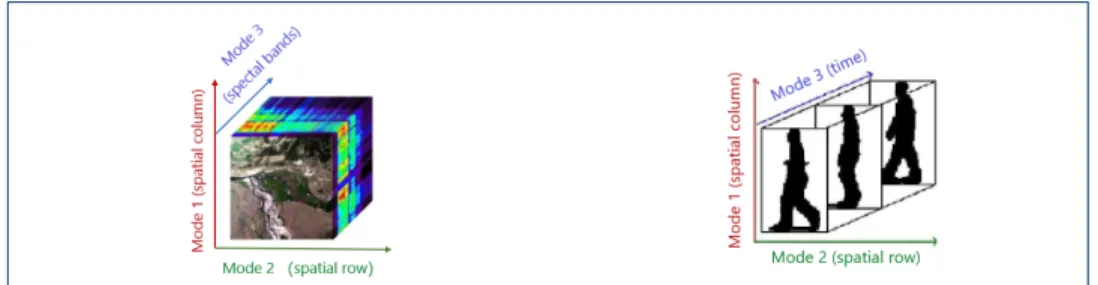
Figure 1: The tensor structure of the multispectral image.
Figure 2: The tensor structure of the video.
sensors to manage, analyze and integrate resources efficiently to provide clearer images to humans. However, multi-source heterogeneous image data analysis is now facing many problems. Complex data objects have multiple dimensions, and how to depict the relationship between them through data analysis is one of the challenges to solve urgently.
For example, we cannot utilize a general matrix to express the spectral image as there are multiple spectral band, (e.g. the mode 3 axis), where each spectral band represents a color image matrix. And we can see that multi-channel images have natural tensor structures from the above case. Moreover, the superposition of image matrix can be seen as a video if the mode 3 axis represents time, and above two tensor structures are shown in Figures 1 and 2. Therefore, tensors can express multiple relationships in the real world, while this paper studies image fusion based on tensor analysis, which can abstractly describe the interaction mechanism between multiple aspects of image data. In addition, tensor structure has strong expression ability and computational properties, so it is very meaningful to study tensor analysis of images. Tensor decomposition is a very significant knowledge content, which can preserve the structural characteristics of the original image data [2].
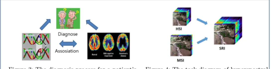
What’s more, multi-source heterogeneous semantics are much more rich. How to build a generalization model that integrates multi-source data or discover the cor-relation between them is another challenge for multi-source heterogeneous images. In this paper, we generally use coupling to refer to the correlation between hetero-geneous images. When doctors make the diagnosis for a patient’s brain, they can get some images of the patient’s brain from a variety of ways, as shown in Figure 3. And whether there is a coupling between these brain images, and how to combine them to determine the etiology of patients are the questions to be discussed in this paper. In addition, for the fusion of hyperspectral images and multispectral images, it aims at integrating the information from them under the same scene, and then generating fused images with more information and higher quality, the goal of this task as shown in Figure 4. Similarly, what is the correlation between the informa-tion contained in these spectral images and how to combine the complementary information to obtain the clearer image are also the significance that this paper need to study.
The outline of this paper is organized as follows. In ”Related work” section, related work about coupled images fusion is discussed. And we mainly describe some basic notations and definitions on tensors in ”Tensor and related notation” section. In
5 6 7 8 9 10 11 12 13 14 15 16 17 18 19 20 21 22 23 24 25 26 27 28 29 30 31 32 33 34 35 36 37 38 39 40 41 42 43 44 45 46 47 48 49 50 51 52 53 54 55 56 57 58 59 60 61 62 63
Figure 3: The diagnosis process for a patient’s brain.
Figure 4: The task diagram of hyperspectral hyper-resolution.
”Coupled image fusion section”, the proposed coupled image fusion algorithms are presented. Moreover, the experimental results on algorithms are shown in ”Exper-iments and results” section. Finally, we give some conclusions and future research directions we need to study next.
Related work
Recently, motivated by the tensor nuclear norm(TNN), Pan Zhou and Canyi Lu proposed a novel low-rank tensor factorization method for efficiently solving the 3-way tensor completion problem, which can recover the synthetic data, inpainting images and videos with superior performance and efficiency [3].For hyperspectral images, tensor decomposition can make full use of space and inter spectral redun-dancy between images, compressing the high spectral image and extracting the related feature information fast and high-quality [4][35-36]. Chia-Hsiang Lin et al proposed a convex optimization-Based coupled nonnegative matrix factorization al-gorithm for hyperspectral and multispectral data fusion [34]. Shutao Li and Renwei Dian proposed a coupled sparse tensor factorization (CSTF)-based approach for fusing hyperspectral images and multispectral images to obtain a high spatial res-olution hyperspectral image[5]. In addition, they consider high spatial resres-olution hyperspectral image (HR-HSI) as a 3D tensor and redefine the fusion problem as the estimation of a core tensor and dictionaries of the three modes[37]. Veganzones and Cohen proposed a Canonical Polyadic decomposition (CP) algorithm based on hyperspectral images, which was used to solve the problem of blind source signal sep-aration [4]. They suggested to solve this problem as a low dimensional constrained tensor decomposition and applied kinds of fast decomposition of large nonnegative tensors which allowed a major speed up in the computation of the decomposition [6].
In the past few years, there have been many researches on the application of CP decomposition in image.In [7] and [38] used the CP decomposition into image com-pression and classification . Marcella Astrid et al used the CP decomposition into Convolutional Neural Networks (CNNs) to solve the image classification tasks [39]. Bauckhage introduced discriminant analysis to higher order data(i.e. color images) for classification [8]. For hyperspectral and multispectral images (i.e. multi-source heterogeneous data), kinds of methods exploits the Bayesian framework [9]-[11] to fuse such images. Rodrigo and Jeremy proposed a Bayesian framework to define flexible coupling models for joint tensor decompositions of multiple datasets[12][40]. They cast the problem of data fusion as the analysis of latent variable. And the la-tent models between data are coupled through subsets of their variables, where the
5 6 7 8 9 10 11 12 13 14 15 16 17 18 19 20 21 22 23 24 25 26 27 28 29 30 31 32 33 34 35 36 37 38 39 40 41 42 43 44 45 46 47 48 49 50 51 52 53 54 55 56 57 58 59 60 61 62 63
coupling refers to the relationship between these variables subset. That is, there is a coupling relationship between the factor matrix after the tensor decomposition. In this paper, we hope to use the coupling relation between images to solve the problem, improving the accuracy and interpretability of the latent variables related to the other data set from the information of one data set through joint tensor decomposition algorithm.
In application, data analysis from different data sources needs to be handled the heterogeneous datasets (i.e. a matrix or a high-order tensor) [13][41]. Recently, matrix factorization and tensor-based factorization have been successfully applied to multi-frame data restoration [14]-[17], recognition [18], [19], unmixing [20] and data fusion [12], etc. For the data analysis of some coupled matrices and tensors, corresponding coupled matrix and tensor factorization-optimization algorithm (i.e. CMTF-OPT) was proposed in [21]. The numerical experiments showed that The CMTF algorithm had better performance than CP algorithm in data recovery at a certain level of noise.
Similarly, the higher order coupled tensor decomposition problem was also studied in [6]. Model showed better performance in coupled tensor decomposition in the ex-periments. Rodrigo and J´er´emy studied the coupling relationship between different data and the data decomposition algorithms under coupling, which showed that the decomposition algorithm based on coupled data had better convergence and the calculation of the algorithm took less time than alternating least squares (ALS) algorithm [12]. So using the coupling relations between images is the necessary mea-sure and work to decompose images. Moreover the algorithms in [12] and [21] are not used to the coupled images. And S. Li and R. Dian do not make full use of the coupling relationship between images and use this coupling relation to accelerate the operation of the algorithm and restore the coupled image data [5]. Therefore, this paper proposes the coupled image data decomposition algorithms based on the CMTF-OPT algorithm [21] and the coupled tensor data decomposition algorithm [12].
Tensor and related notation
In the nineteenth century, Gauss and Riemann put forward the concept of tensors in the study of differential geometry. In 1916, Einstein applied tensors to the study of the general relativity, which made tensor analysis to be an important tool in con-tinuum mechanics, theoretical physics and other disciplines. In 2005, characteristic polynomial was proposed for the first time in real symmetric tensor by Qi Liqun, and he presented the definition of the eigenvalues [22].
In order to study the data fusion between the coupled images better and sim-plify the presentation, this paper first introduces some of the following symbols and definitions. For the general tensor, this paper uses the calligraphic letters to rep-resent them e.g. X, the matrix is denoted by capital letters e.g.X, and the scalar (or. vector) is represented by lowercase, e.g.x. The mode-nmatricization of a ten-sor X ∈ RI1×I2×···×IN is denoted byX
(n), which can reduce the dimension of the
tensor.For a matrix A∈ RI×J, vectorization is to expand the matrix by column, 5 6 7 8 9 10 11 12 13 14 15 16 17 18 19 20 21 22 23 24 25 26 27 28 29 30 31 32 33 34 35 36 37 38 39 40 41 42 43 44 45 46 47 48 49 50 51 52 53 54 55 56 57 58 59 60 61 62 63
forming aIJ Column vector, that is vec(A) = a1 .. . aJ ∈RIJ. (1)
Given two matricesA∈RI×KandB∈RJ×K, the Khatri-Rao product is denoted
as AB, and the calculation results is a matrix of size IJ×K and defined by
AB= [a1⊗b1 a2⊗b2 · · · aK⊗bK], (2)
where ⊗is the Kronecker product.
Given two tensorsA,B ∈RI1×I2×···×IN, the Hadmard product denoted asA ∗ B,
and the calculation results is a matrix of size I×J, i.e.
A ∗ B= a11b11 a12b12 · · · a1Jb1J a21b21 a22b22 · · · a2Jb2J .. . ... . .. ... aI1bI1 aI2bI2 · · · aIJbIJ . (3)
Given two tensors A,B ∈RI1×I2×···×IN,the inner product is defined as the sum
of the product of its elements, i.e.
hA,Bi= I1 X i1=1 I2 X i2=1 · · · IN X iN=1 xi1i2···iNyi1i2···iN, (4)
we usually use ’◦’ to represent the outer product.
Let matrix A= (aij)m×n∈ Cm×n, the Frobenius norm is defined as
kAkF= ( m X i=1 n X j=1 |aij|2) 1 2. (5) Tensor decomposition
In applications, the general tensor decomposition models can be divided into two categories, which are the Canonical Polyadic/PARAFAC decomposition (e.g. CP decomposition) and the Tucker decomposition model. The canonical decomposition was originally proposed by Carroll and Chang [23] and PARAFAC (parallel factors) by Harshman [24] separately. In 1966 Tucker [25] proposed the Tucker model. In particular, the CP decomposition model is a special case of the Tucker decompo-sition model.At the time, models were put forward to extract data characteristics from psychological tests. For the general matrix model, we can extract the poten-tial information of matrix data, such as hyperspectral data fusion and blind source separation, by means of singular value decomposition of matrix, nonnegative ma-trix decomposition and so on. Similar to the idea of low rank approximation of matrix, researchers also want to extract latent information from tensor model data
5 6 7 8 9 10 11 12 13 14 15 16 17 18 19 20 21 22 23 24 25 26 27 28 29 30 31 32 33 34 35 36 37 38 39 40 41 42 43 44 45 46 47 48 49 50 51 52 53 54 55 56 57 58 59 60 61 62 63
by means of tensor decomposition model.
For a tensor X ∈RI1×I2×···×IN,the CP decomposition is expressed as
X ≈ R X r=1 λra(1)r ◦a (2) r ◦ · · · ◦a (N) r = [[λ;A (1) ,A(2),· · ·,A(N)]], (6) whereRis a positive integer,A(n)is called the factor matrix, which is a combination
of rank one vectora(rn),e.g.
A(n)= [a(1n), a2(n),· · · , a(Rn)], (7) forn= 1,2,· · · , N,λ∈RR,a(rn)∈RIn,A(n)∈
RIn×R.
Especially, for the three order tensor X ∈RI×J×K,the CP decomposition is
ex-pressed as X ≈ R X r=1 λrar◦br◦cr= [[λ;A,B,C]], (8) where r= 1,2,· · ·, R, λ∈RR,a r∈RI,br∈RJ,cr∈RK.
Here, the column of factor matrix A,B andC is normalized to 1, andλr is the
weight. If the weight is assigned to the factor matrix, the CP decomposition can also be showed as
X ≈(A0,B0,C0). (9)
Now we define Dr composed of λr is R×R×R order diagonal tensor, so the
equation can be transformed into
X = (A,B,C)· Dr. (10)
Coupled image fusion
Coupled data fusionData fusion, also known as collective data analysis, has been a hot topic in different fields. Data analysis from multiple sources has attracted considerable people in the Netflix Grand Prix. The goal is to accurately predict movie ratings. In order to get better ratings, additional data sources supplement the user score, such as the label information has been used. And the collective matrix factorization (CMF) proposed by Singh and Gordon [26] is based on the correlation between data sets, and the coupling matrix is factored simultaneously. Many researchers have paid their more attention to image fusion technique based on pulse coupled neural net-work. Literature [31] described the models and modified ones. As to the multi-focus image fusion problem, Farshad G. Veshki et al. utilized the sparse representation using a coupled dictionary to address the focused and blurred feature problem for higher quality[32]. In order to create spectral images with high spectral and spatial resolution, Yuan Zhou et al [33] proposed a fusion algorithm by combining linear spectral unmixing with the local low-rank property by extracting the abundance
5 6 7 8 9 10 11 12 13 14 15 16 17 18 19 20 21 22 23 24 25 26 27 28 29 30 31 32 33 34 35 36 37 38 39 40 41 42 43 44 45 46 47 48 49 50 51 52 53 54 55 56 57 58 59 60 61 62 63
and the endmembers of Hyperspectral images usually have high spectral and low spatial resolution. Conversely, multispectral images.
For two matrices X∈RI×M,Y∈RI×L, the general CMF decomposition model
is established by minimizing the following objective function f(U,V,W) =kX−UVTk2
F+kY−UWTk2F, (11)
where the matricesU∈RI×R,V∈RM×RandW∈RL×Rare the factor matrices,
Ris the number of factors. In particular, because there exists a large number of high-order data, the data fusion between the coupled tensor and the matrix is discussed below.
For a tensor X ∈RI×J×K and a matrix Y ∈RI×M, the general coupled tensor
and matrx decomposition model is established by modifying the above objective function f(A,B,C,V) =k X −(A,B,C)k2 F+kY−AV T k2 F, (12)
where the matrices A ∈ RI×R, B ∈ RJ×R and C ∈ RK×R are factor matrices
obtained by CP decomposition of the tensor X.
Alternating Least Squares Algorithm for coupled matrix and tensor factorization (CMTF-ALS) algorithm is proposed in [21]. The algorithm based on ALS is simple, small and effective. However, the convergence of the algorithm based ALS is not good with the missing data [27]. On the other hand, it is more robust to solve all CP factor matrices with an optimized algorithm, and is more easily extended to the missing data set [28]. Therefore, for high order data sets, with the support of the algorithm proposed in [21], this paper presents some coupled image decomposition algorithms, which describe the coupling analysis of heterogeneous image data sets.
Coupled tensor decomposition algorithm CIF-OPT algorithm
The main purpose of this paper is exploring data fusion between coupled im-ages. In general, images are stored in terms of tensor or matrix. Based on the CMTF optimization(CMTF-OPT) algorithm in [21], a coupled images factorization-optimization(CIF-OPT) algorithm is proposed. We firstly consider matrix image and N-order tensor image with one mode in common, where tensor image is de-composed through CP model and matrix image is dede-composed through matrix decomposition.
Given a tensor image X ∈RI1×I2×···×IN and a matrix imageY∈
RI1×M which have have the nth mode in common, wheren∈ {1,· · ·, N}. Without loss of gener-ality, we assume that two images coupled in the third mode, and the common latent structure in these images can be extracted by CIF-OPT algorithm. The objective function of the coupled analysis between the two image datasets is as follow
f(A(1),A(2),· · · ,A(N),V) =k X −[[A(1),A(2),· · ·,A(N)]]k2 F+kY−A (n)VTk2 F, (13) 5 6 7 8 9 10 11 12 13 14 15 16 17 18 19 20 21 22 23 24 25 26 27 28 29 30 31 32 33 34 35 36 37 38 39 40 41 42 43 44 45 46 47 48 49 50 51 52 53 54 55 56 57 58 59 60 61 62 63
In order to solve the above optimization problem, we can calculate its gradient and solve it by using any first order optimization algorithm of [29]. Next, this paper will discuss the gradient of the objective function,the first item of the function (12) is written as
f1=k X −[[A(1),A(2),· · · ,A(N)]]k2F, (14)
the second item of the function (12) is recorded as
f2=kY−A(n)VTk2F. (15)
LetS = [[A(1),A(2),· · ·,A(N)]],and the specific forms of the partial derivative of
f1with respect to A(i)are as below
∂f1
∂A(i) = (S(i)−X(i))A
(−i), (16)
where i= 1,2,· · ·, N.The matricesAand V∈RM×Rare factor matrices obtained
by matrix decomposition of the matrix Y.
A(−i)=A(N) · · · A(i+1)A(i−1)A(1). (17) The specific forms of the partial derivative off2 with respect toA(i) andVcan
be computed as ∂f2 ∂A(i) = ( −YV+A(−i)VTV, f or i=n, 0, f or i6=n. (18) ∂f2 ∂V =−Y TA(i)+VA(i)TA(i). (19)
Combined with the above calculation results, we can calculate the objective func-tionf. ∂f ∂A(i) = ∂f1 ∂A(i)+ ∂f2 ∂A(i), ∂f ∂V = ∂f2 ∂V =−Y TA(i)+VA(i)T A(i). (20)
Finally, this paper calculates the gradient of the optimization functionf, and its specific form is a vector e.g.
∇f = vec(∂A∂f(1)) .. . vec(∂A∂f(N)) vec(∂∂fV) . (21)
where the length of the vector is P =RPN
n=1(IN +M), which can be formed by
vectorizing the partial derivatives with respect to each factor matrix and forming a column vector. 5 6 7 8 9 10 11 12 13 14 15 16 17 18 19 20 21 22 23 24 25 26 27 28 29 30 31 32 33 34 35 36 37 38 39 40 41 42 43 44 45 46 47 48 49 50 51 52 53 54 55 56 57 58 59 60 61 62 63
For some missing data sets, coupling analysis can still be carried out. The imple-mentation of the algorithm can ignore missing data, and only analyze the known data elements to find the tensor or matrix model. And we applied it to the miss-ing image and restored the original image based on the proposed coupled image decomposition algorithm through the another coupled image, which refer to [21].
Flexible coupling models
Rodrigo and J´er´emy proposed the flexible coupling models based on the joint de-composition of Bayesian estimation in [12]. They mainly present two general exam-ples of coupling priors such as joint Gaussian priors and non Gaussian conditional distributions. For two tensors with noisy measurements Y and Y0, Y is a second tensor(e.g. matrix) which can be the SVDY=UΣVT+E, andY0 is a third order tensor which can be written Y0 = (A0,B0,C0) +ε0 via CP decomposition,where E
andε0 are the noisy array.
Letθ= vec([U;Σ;VT]) andθ0 = vec(A0;B0;C0). Here we assume the parameters θ andθ0 are random and consider that the coupling between them is flexible, for instance, we could have V=B, orV=WB for a known transformation matrix
W. Under the some simplifying hypotheses underlying the Bayesian approach, the Maximum a posteriori estimator(MAP) estimator is given as the minimizer of the following cost function
arg min
θ,θ0
Υ(θ, θ0) =−logp(Y |θ)−logp(Y0 |θ0)−logp(θ, θ0). (22)
where p(θ, θ0) is the joint probability density function,p(Y |θ) and p(Y0 |θ0) are the conditional probabilities.
Given two CP models Y = (A;B;C) and Y0 = (A0;B0;C0) with dimensions I, J,KandI0,J0,K0 and number of components (i.e. number of matrix columns)R and R0 respectively. Considering the coupling occurs between matricesC andC0. Rodrigo and J´er´emy illustrate this framework with three different examples: general joint Gaussian, hybrid Gaussian and non Gaussian models for the parameters in [12]. This paper only discusses the second example (e.g. the hybrid Gaussian model), and the other two cases are not considered by us. If readers are interested, you can refer to the literature [12].
If there is no prior information about some parameters, the joint Gauss modeling is not enough. On the contrary, we consider that these parameters are deterministic, while other parameters are still random Gauss priors. We call this model a hybrid Gaussian model. In fact, it only covers one scene which is factor matrixCis coupled to C0 another by a transformation matrix, this coupled relation can be written by
HC=H0C0+Γ, (23)
where Hand H0 are transformation matrices,Γ is noisy of independent and iden-tically distributed (i.i.d.) Gaussian with matrix C, e.g.Γ∼N(0, σ2c).
Under the assumption of hybrid Gaussian model[5], the MAP estimation is ob-tained by minimizing the following cost function, that is, transforming function (22)
5 6 7 8 9 10 11 12 13 14 15 16 17 18 19 20 21 22 23 24 25 26 27 28 29 30 31 32 33 34 35 36 37 38 39 40 41 42 43 44 45 46 47 48 49 50 51 52 53 54 55 56 57 58 59 60 61 62 63
into Υ(θ, θ0) = 1 σ2 n k Y−(A,B,C)k2 F+ 1 σ02 n k Y0−(A0,B0,C0)k2 F+ 1 σ2 c kHC−H0C0k2 F, (24)
a. Hybrid gaussian modeling and alternating least squares(ALS) algorithm
To minimize the above objective functions, standard algorithm matched with con-vex optimization can be used, Rodrigo and J´er´emy proposed the modified version of the alternating least squares(ALS) which is widely used and easy to implement. We will refrain on detailing above algorithms.
Using the above algorithm to initialize the original tensor, the factor matrices are generated randomly and the tensor is formed by the tensor product operation between the factor matrices. Finally, we can estimate the effectiveness of the algo-rithms by comparing the mean square error between the factor matrices obtained by the above coupling tensor decomposition algorithms of the noisy tensor and the original factor matrices. If we apply the above algorithms to image, we need to initialize the original image, that is, generating the original factor matrices. In this paper, we use the following algorithm(i.e. Algorithm 1) to generate coupled images. In this paper, the ALS algorithm is used to initialize the image, we modify the objective function and algorithm in [12] as follows:
Υ(θ, θ0) = 1 σ2 n k Y −(A,B,C)· Drk2F+ 1 σ02 n k Y0 −(A0,B0,C0)· D0rk2 F+ 1 σ2 c kHC−H0C0 k2 F, (25)
In order to apply ALS algorithm, it’s necessary to calculate its gradient with respect to every factor matrix and set it to zero. For coupled factorsCandC0, this algorithm only considers updating them simultaneously, which requires to solve the following linear equations[5]:
Mvec([C;C0]) = vec([ 1 σ2 n Y(3)D; 1 σ02 n Y(3)0 D0]), (26) whereM= [M11,M12;M21,M22],D= (BA)T(BA),D 0 = (B0A0)T(B0A0) and M11= 1 σ2 c IR⊗HTH+ 1 σ2 n DT⊗IK, M22= 1 σ2 c IR⊗H 0T H0+ 1 σ02 n D0T⊗IK, M12=− 1 σ2 c IR⊗HTH 0 , M21=− 1 σ2 c IR⊗H 0T H. (27)
b. Joint tensor decomposition of high dimensional coupled images 5 6 7 8 9 10 11 12 13 14 15 16 17 18 19 20 21 22 23 24 25 26 27 28 29 30 31 32 33 34 35 36 37 38 39 40 41 42 43 44 45 46 47 48 49 50 51 52 53 54 55 56 57 58 59 60 61 62 63
Algorithm 1. Algorithm for generating coupled images
step1:For two images, reading the image data with the image reading function(Im2double) in MATLAB to generate the tensorX, X0.
step2:Applying CP decomposition algorithm (CP-ALS) to obtainaˆ0,
ˆb0,ˆc0,Dr,aˆ0 0,ˆb 0 0,cˆ 0 0,D 0 r.
step3:For simplification, absorbing the diagonal tensorDrandD
0 rin ˆ a0 andˆa 0 0to obtainAˆ0 andAˆ 0
0. Using the coupling factorσc andCˆ0
to initial factor matricCˆ00 , e.g.
ˆ
C00 = ˆc0+σc∗(γa, Rb);
step4:Using tensor product forAˆ0,ˆb0, ˆc0 andAˆ 0 0,ˆb 0 0,Cˆ 0 0 to obtain
new tensors. Then the noise is added to the tensors to have coupled imagesY,Y0.
aThis footnote is a zero mean white Gaussian matrix. bThis footnote is the rank in tensor decomposition.
For the actual high-dimensional images, a high dimensional coupled image decom-position algorithm is proposed. It is assumed that the coupling relationship between images is as follow:
C=C0 + Γ, (28)
where Γ is an i.i.d. Gaussian matrix with variance of each element σ2
c andC
0
has columns of given norm. If we disregard the coupling of the tensors, a common method to retrieve the CP models is to compress the data arrays, decomposing the compressed tensors, and then uncompress the obtained factors matrices, which is a more computationally efficient way.
For a three-order tensorX ∈RI×J×K,the tucker decomposition is expressed as X ≈ P X p=1 Q X q=1 R X r=1 gpqrup◦vq◦wr= [[G;U,V,W]], (29)
where U ∈RI×P,V∈ RJ×Q, andW ∈RK×R are the factor matrices ,which are
usually orthogonal.The positive integersP,Q, andRare the number of components (i.e., columns) in the factor matrices U, V, and W, respectively. The tensor G ∈ RP×Q×R is called the core tensor. Tucker decomposition is a high-order principal
component analysis, which represents a tensor as a core tensor multiplied by a matrix along each mode.
If we assume two tensors are noiseless, i.e.
X ≈ P X p=1 Q X q=1 R X r=1 gpqrup◦vq◦wr= (U,V,W)G, X0≈ P0 X p=1 Q0 X q=1 R0 X r=1 g0pqru0p◦vq0 ◦wr0 = (U0,V0,W0)G0, (30)
In this section, we consider the decomposition algorithm of the coupled high di-mensional images. The high didi-mensional image is decomposed into the low
5 6 7 8 9 10 11 12 13 14 15 16 17 18 19 20 21 22 23 24 25 26 27 28 29 30 31 32 33 34 35 36 37 38 39 40 41 42 43 44 45 46 47 48 49 50 51 52 53 54 55 56 57 58 59 60 61 62 63
sional core tensor through the Tucker decomposition, and then decomposing the two core tensors by CP decomposition to get the factor matrices, the compressed CP models will reduce the cost and consumption of the calculation. There exists the relationship below.
G ≈(Ac,Bc,Cc),G 0 ≈(A0c,B 0 c,C 0 c), (31)
The factor matrix of the original tensor can be solved by matrix multiplication with less computation.
(U,V,W)G= (UAc,VBc,WCc),A=UAc,B=VBc,C=WCc (32)
It is assumed that the coupling relationship between noiseless tensors in the com-pressed space as
WCc =W
0
C0c+ Γ (33)
However, if one tensor is noisy(i.e. Y),there exists the similarity coupling in the compressed dimension
Cc=C
0
c+ Γc (34)
where Γc is a matrix of same dimensions asCc and with Gaussian i.i.d. entries of
variance. The hybrid objective function in the compressed space is modified to the following objective function,which can be solved using the ALS algorithm.
Υ(θ, θ0) = 1 σ2 n k G−(Ac,Bc,Cc)k2F+ 1 σ02 n k G0−(A0c,B0c,C0c)k2 F+ 1 σ2 c kCc−C 0 c k 2 F, (35)
For the factorization of some coupled images, we expect that the factor matrices obtained by factorization algorithm can be shown by images. That means to min-imize the objective function under the constraint of nonnegative conditions. The MU algorithm is usually used for nonnegative matrix factorization [6].
Experiments and results
The main idea of this paper is applying the above coupled data fusion algorithms to deal with the image. It is well known that the stored data values of images are ordinarily large. If the tensor decomposition algorithm is applied directly to the coupled image data, the error is a big problem, which makes us use the command Im2doublein Matlab to scale the values to reduce the numerical error in program operation.
CIF-OPT algorithm
In this section, the coupled matrix tensor decomposition method is applied to mul-tispectral and panchromatic images. The original images which are the low spatial
5 6 7 8 9 10 11 12 13 14 15 16 17 18 19 20 21 22 23 24 25 26 27 28 29 30 31 32 33 34 35 36 37 38 39 40 41 42 43 44 45 46 47 48 49 50 51 52 53 54 55 56 57 58 59 60 61 62 63
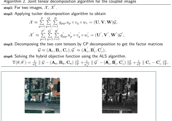
Algorithm 2. Joint tensor decomposition algorithm for the coupled images
step1:For two images,X,X0.
step2:Applying tucker decomposition algorithm to obtain X ≈ P P p=1 Q P q=1 R P r=1 gpqrup◦vq◦wr= (U,V,W)G, X0 ≈ P0 P p=1 Q0 P q=1 R0 P r=1 gpqr0 u 0 p◦v 0 q◦w 0 r= (U 0 ,V0,W0)G0,
step3:Decomposing the two core tensors by CP decomposition to get the factor matrices G ≈(Ac,Bc,Cc),G
0
≈(A0c,B0c,C0c),
step4:Solving the hybrid objective function using the ALS algorithm.
Υ(θ, θ0) =σ12 n k G −(Ac,Bc,Cc)k 2 F+ 1 σ02 n k G0−(A0c,B0c,C0c)k2 F+ 1 σ2 c kCc−C 0 c k2F,
Figure 5: The multispectral image of area I Figure 6: The panchromatic image of area I
resolution multispectral image located in Beijing, China and the corresponding high spatial resolution panchromatic image are as follows.
The experimental data are captured from Airborne Visible Infrared Imaging Spectrome-TER (AVIRIS) in Beijing. The AVIRIS data can provide 224 spectral segments with a spatial resolution of 20m, covering a spectral range of 0.2∼2.4m, and its spectral resolution is 10nm. The size of multispectral and panchromatic im-ages of area I which are shown in Fig.5 and Fig.6 are 300×300×3 and 300×300 pixels respectively. The size of multispectral and panchromatic images of area II which are shown in Fig.7 and Fig.8 are 256×256×3 and 256×256 pixels respectively. The multispectral and panchromatic image data of area I are read and initialized by MATLAB, and stored as tensorX ∈R300×300×3and matrixY∈
R300×300. And
the tensors of area II are generated in the same way.
According to the data generation of the CIF-OPT algorithm, the original data are sampled from the multispectral and panchromatic images, and the initial factor matrix is obtained by the ALS algorithm. Using the tensor product and the matrix multiplication to calculate the noiseless initial tensor and matrix. Without losing generality, we set the coupled factor matrix between tensor and matrix to C. In order to study the performance of the algorithm better, experiments are carried out under different noise levels.
Adding noise to the obtained tensorX ∈R300×300×3and the matrixY∈R300×300
after initializing the images, e.g.
X0= [[A,B,C]] +ηNk[[A,B,C]]k kN k , (36) 5 6 7 8 9 10 11 12 13 14 15 16 17 18 19 20 21 22 23 24 25 26 27 28 29 30 31 32 33 34 35 36 37 38 39 40 41 42 43 44 45 46 47 48 49 50 51 52 53 54 55 56 57 58 59 60 61 62 63
Figure 7: The multispectral image of area II Figure 8: The panchromatic image of area II
where N ∈R300×300×3is the stochastic Gaussian noise tensor,η is used to control
the noise level. Similarly, the Gaussian noise is added to the matrixY, that is,
Y0 =AVT+ηNkAV
Tk
kNk , (37)
whereN∈R300×3 is the stochastic Gaussian noise matrix,η is used to control the
noise level.
In this experiment, four different noise levels are set, which are 0, 0.1, 0.25, and 0.35 respectively. As the terminating condition of the CIF-OPT algorithm, it needs to be satisfied
5f = |fk+1−fk| fk
≤10−8, (38)
where f is the objective function, in addition, the maximum number of function values and iteration number is set to 104and 103respectively. In the process of ex-periment, the termination condition of algorithm depends on the change of function value before and after iteration.
The main purpose of this section is to apply the CIF-OPT algorithm to the cou-pled multispectral and panchromatic images and the specific results are shown in Table 1. From Table 1, it can be seen that the CIF-OPT algorithm has the similar fusion effect for different images, which shows that the algorithm has a certain ro-bustness. The fusion effect will not change dramatically as the vary of image order and data elements. Moreover, the number of iterations does not alter greatly with the increase of order, which proves the feasibility of decomposition for coupled im-ages.
Table 1: Comparison of decomposition algorithms on different areas
η Area Iter FuncEvals f
0.10 1 521 1073 0.0098158 2 942 2693 0.0097922 0.25 1 842 1702 0.0583453 2 302 632 0.0581043 0.35 1 442 924 0.1080817 2 422 883 0.1077908
The change from coupled data to the coupled image decomposition algorithm shows the iteration times and the maximum number of functions that CIF-OPT
5 6 7 8 9 10 11 12 13 14 15 16 17 18 19 20 21 22 23 24 25 26 27 28 29 30 31 32 33 34 35 36 37 38 39 40 41 42 43 44 45 46 47 48 49 50 51 52 53 54 55 56 57 58 59 60 61 62 63
0.1 0.15 0.2 0.25 0.3 0.35
Different noise levels
0 0.02 0.04 0.06 0.08 0.1 0.12
Target function value
CMTF-OPT algorithm ACMTF algorithm
Figure 9: Comparison of objective function values under different noise levels.
0 0.1 0.2 0.3 0.4 0.5
Different noise levels
0 0.02 0.04 0.06 0.08 0.1 0.12 0.14 0.16 0.18 0.2
Target function value
CIF-OPT algorithm AICT algorithm
Figure 10: Comparison of objective function values under different noise levels.
algorithm needs to convergence is larger than CMTF-OPT algorithm. The results are inevitable, because the coupled image needs to be initialized and converted to the coupled data to achieve the algorithm when the coupled image is decomposed. Therefore, the convergence of algorithm requires more iteration times. Accordingly, by observing the experiment of adding noise to the coupled image, it can be seen that the proposed algorithm can realize the decomposition of the coupled image, and the decomposition effect is better than the CMTF-OPT algorithm under the certain noise level. Consequently, the above results prove the feasibility of coupled image decomposition.
Another ACMTF algorithm for coupling image decomposition conducted the same noise level experiment for region I, and compared with CMTF-OPT algorithm. The results are shown in Fig. 9. It can be seen that ACMTF algorithm is superior to CMTF-OPT algorithm in different noise levels. Therefore, based on the same param-eters and noise conditions, this paper conducts the same noise level experiment for another ACIF algorithm of coupled image, and compares the target function value, iteration times, error and other parameter results between the two algorithms. The fusion effect under different noise levels is shown in Fig. 10. Experimental results show that CIF-OPT algorithm is more effective than ACIF algorithm when the added noise is less than 0.2. This is different from the data fusion effect of the two algorithms in the coupled data, and with the increase of noise level, the perfor-mance of the two algorithms in the fusion effect is almost the same, which shows that the improved image decomposition algorithm does not have better advantages than CIF-OPT algorithm.
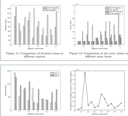
In this paper, the number of iterations required for algorithm convergence is com-pared as shown in Fig. 11. It can be seen from Fig. 11 that the number of iterations required for ACIF algorithm to converge is more than CIF-OPT algorithm in most cases, and the running time from reaching convergence condition to algorithm ter-mination is longer when the algorithm is running. In order to comprehensively con-sider various factors, this paper calculates the fusion errors of the four algorithms to comprehensively compare the accuracy of the algorithm for data decomposition. See Fig. 12 for the specific results.
Fig. 12 shows that to some extent, the decomposition effect of the coupled image is better than that of the coupled data, but the error of the decomposition algorithm
5 6 7 8 9 10 11 12 13 14 15 16 17 18 19 20 21 22 23 24 25 26 27 28 29 30 31 32 33 34 35 36 37 38 39 40 41 42 43 44 45 46 47 48 49 50 51 52 53 54 55 56 57 58 59 60 61 62 63
Figure 11: Comparison of iteration times in different regions.
Figure 12: Comparison of the error values in different noise levels.
Figure 13: The coupled imageX.
0 0.1 0.2 0.3 0.4 0.5 0.6 0.7
Different noise levels 0 0.2 0.4 0.6 0.8 1 1.2 1.4 1.6 1.8
The difference of objective values in different regions
10-5
Figure 14: The coupled imageX0.
of the coupled data has a certain stability, and the error difference is lower than that of the decomposition algorithm of the coupled image. For the two algorithms of coupled image decomposition, when the noise level is lower than 0.25, the error value of the two algorithms is unstable, and the error value of Fig. 12 is small. Therefore, with the increase of noise level, the error value of CIF-OPT algorithm is very close to that of ACIF algorithm. So for the coupled image decomposition algorithm, CIF-OPT algorithm shows better fusion effect at low noise level, and the error difference and the number of iterations required for algorithm convergence are less.
The above algorithm is mainly based on the comparison of the result parameters of region I. We compare the iterations of the algorithm and the difference between the objective function values for two different regions based on CIF-OPT algorithm, and the results are shown in Fig. 13 and Fig. 14. It can be seen that there is no obvious linear relationship between the number of iterations and the image size. Because the magnitude of figure 14 is very small, the objective function values of the two regions are very close, that is to say, the function optimal value of CIF-OPT algorithm will not change significantly due to the difference of image size and pixel. Based on the proposed CIF-OPT optimization algorithm, the multispectral images of the missing data coupled with the panchromatic image are restored. That is, all
5 6 7 8 9 10 11 12 13 14 15 16 17 18 19 20 21 22 23 24 25 26 27 28 29 30 31 32 33 34 35 36 37 38 39 40 41 42 43 44 45 46 47 48 49 50 51 52 53 54 55 56 57 58 59 60 61 62 63
-0.01 -0.005 0 0.005 0.01 0.015 0.02 True value -0.01 -0.005 0 0.005 0.01 0.015 Estimated value
Figure 15: Data estimation with 25% missing data.
Figure 16: Data estimation with 50% missing data.
Figure 17: The uncoupled original image.
the data of the panchromatic image are known. The specific results of the algorithm are shown in Fig.15 and Fig.16. Where the missing data of this experiment occurred in area II and the recovered data is the transformed data, not the original image data. By observing the data curve recovered by the CIF-OPT algorithm, it is known that the data recovery effect of the coupled image with 25% missing data is better than the effect of image with 50% missing data. That is, the correlation between real value and estimated value is stronger when the percentage of missing data is 25%, and the linear slope is closer to 1.
Straightforward hybrid Gaussian coupled decomposition
We consider the straightforward hybrid Gaussian coupling modelC=C0+Γ. And we select the small images inside the red frame as the uncoupled original tensors of Algorithm 1 in Fig.17. The two CP models are generated by these images with dimensionsI =I0 =J =J0 = 30, K=K0 = 3 and R=R0 = 8, e.g.Y,Y0. Then through simplification and adding Gaussian noise and different coupling intensity to Y,Y0 to obtain the new tensors Y,Y0
.The original tensor images are shown in Fig.18 and Fig.19. And the new tensor Y is almost noiseless σn = 0.001, while Y
0
has some noiseσ0n= 0.1. The coupled images were generated by Algorithm 1, and decomposed by the ALS algorithm(i.e. Alg. 1) in [5]. Alg. 1 is applied to estimate
5 6 7 8 9 10 11 12 13 14 15 16 17 18 19 20 21 22 23 24 25 26 27 28 29 30 31 32 33 34 35 36 37 38 39 40 41 42 43 44 45 46 47 48 49 50 51 52 53 54 55 56 57 58 59 60 61 62 63
Figure 18: The coupled imageY.
Figure 19: The coupled imageY0.
the CP models under 400 different noise and coupling realizations. We also evaluate the total MSE on the C andC0 factors and the total MSE for an ALS algorithm. And the total MSE on a factor, for example the total MSE onCwithNr different
noise realizations is (1/Nr)PKk=1PRr=1PnN=1r (Ckr−Cˆnkr)2, where ˆCnkr is the factor
estimated in the n-th noise realization.
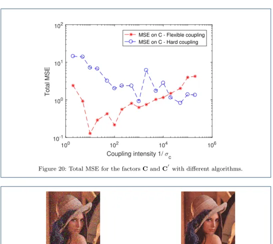
Due to the different coupling intensity of the image, we used the above algorithms to decompose the image and get the mean square error of the factor matrix C for different coupling intensity. We can see that the factor matrix is generally better estimated by increasing the coupling density while applying a hard coupling(i.e.
C=C0) in Fig.20, since more information comes from the clean tensor through the coupling. For a flexible coupling,instead of the mean square error decreases while 1/σc >102. And in the interval 1/σc ∈ [10; 104], the flexible coupling model has
better estimation performance than the hard couplings. For 1/σc>104, the flexible
couplings works better than a hard coupling.
Compressed coupled decomposition
For high-dimensional images, the compressed data decomposition algorithm is adopted in this paper. The selected images are the Lena noised images which are as follows in Fig.21 and Fig.22. The tensors are generated by the following two images with dimensions I =I0 =J =J0 = 256,K =K0 = 3 and P = 50, Q= 40. For the coupled compression decomposition algorithm of large images, the number of
5 6 7 8 9 10 11 12 13 14 15 16 17 18 19 20 21 22 23 24 25 26 27 28 29 30 31 32 33 34 35 36 37 38 39 40 41 42 43 44 45 46 47 48 49 50 51 52 53 54 55 56 57 58 59 60 61 62 63
100 102 104 106 Coupling intensity 1/ c 10-1 100 101 102 Total MSE
MSE on C - Flexible coupling MSE on C - Hard coupling
Figure 20: Total MSE for the factorsCandC0 with different algorithms.
Figure 21: The coupled imageX. Figure 22: The coupled imageX0.
decomposed components is not well defined. Therefore, under the condition of the same coupling density (1/σc = 103), we selected the best number of components
based on the MSE on factor matrix C. The experimental results are shown in Fig.23, which showed that the mean square error of factor matrix is the smallest when R = 3. So later in this paper, R = 3 as the best number of components is used for other experiments. Factor matrices are generated by CP decomposition algorithm similarly to the previous example. The matix C is coupled with factor matrixC0 with additive zero mean Gaussian noise of varianceσ2
c. Where
σc=|
det(C0−C)
det(γ, R) |, (39)
and γis a zero mean white Gaussian matrix. The data arrayY is almost noiseless σn = 0.001, whileY
0
has some noise σn0 = 0.1.We compare the performance of the coupled algorithm in the compressed space and the uncompressed space.Results for 20 iterations of the coupled algorithms are shown in fig.24 and fig.25. Compression was computed with randomized SVD from [30]. And initializations were given by two coupled uncompressed ALS with 1000 iterations, themselves initialized by de-composing images.
As shown in the picture, the compression and ALS algorithms show similar performance in the case of coupling, and the decomposition accuracy of the two
5 6 7 8 9 10 11 12 13 14 15 16 17 18 19 20 21 22 23 24 25 26 27 28 29 30 31 32 33 34 35 36 37 38 39 40 41 42 43 44 45 46 47 48 49 50 51 52 53 54 55 56 57 58 59 60 61 62 63
0 1 2 3 4 5 6 7 8 9 10 Components 0 0.5 1 1.5 2 2.5 3 3.5 4 4.5 5 5.5 6 6.5 7 Average MSE on C ALS
coupled uncompressed ALS coupled compressed ALS
Figure 23: Decomposition performance of three algorithms under different ranks .
0 0.5 1 1.5 2 2.5 3 3.5 4 4.5 Coupling intensity 105 2 4 6 8 MSE
Figure 24: Total MSE for the factorsCandC0 in the compressed space.
0 0.5 1 1.5 2 2.5 3 3.5 4 4.5 Coupling intensity 105 2 4 6 8 MSE
Figure 25: Total MSE for the factorsCandC0 in the uncompressed space.
algorithms decreases with the increase of the coupling density.
Then we study the relationship between noise and algorithm estimation perfor-mance. The SNR for Y is set to 22 dB, and it varies from 4 dB to 20 dB for
Y0.Where SNR(Y) = 10log10 R(1 +σc2) IJ σ2 n ,SNR(Y0) = 10log10 R I0 J0 σ02 n . (40)
We compare the performance of the coupled algorithm in the compressed space and the uncompressed space, as well as standard ALS in the uncompressed space. Note that in Fig.26,When the SNR<18dB, uncoupled ALS algorithm works better
5 6 7 8 9 10 11 12 13 14 15 16 17 18 19 20 21 22 23 24 25 26 27 28 29 30 31 32 33 34 35 36 37 38 39 40 41 42 43 44 45 46 47 48 49 50 51 52 53 54 55 56 57 58 59 60 61 62 63
4 6 8 10 12 14 16 18 20 SNR(Y) 0 1 2 3 4 5 MSE on C ALS
coupled uncompressed ALS coupled compressed ALS
Figure 26: Reconstruction MSE of noisy factorC0 with different algorithms.
0 1 2 3 4 Coupling intensity 105 0.0425 0.043 0.0435 0.044 0.0445 Time
Figure 27: Computation time in the compressed space.
0 0.5 1 1.5 2 2.5 3 3.5 4 4.5 Coupling intensity 105 0.31 0.315 0.32 0.325 Time
Figure 28: Computation time in the uncompressed space.
than the remaining two algorithms.As the noise level increases,for SNR>18dB,the uncoupled ALS algorithm decreases estimation performance in both coupled and compression cases.
On the run time of the algorithm, Fig.27 and Fig.28 show the clear difference in computation time between kinds of decomposition algorithms. We can see that the compression decomposition algorithm obviously saves time and cost compared to the uncompressed algorithm which may be rather slow. As the noise level increases, uncoupled ALS decreases estimation performance in both coupled and compression cases. In addition, hybrid coupling model is only verified in Gaussian condition to show its effectiveness and we will do other experiments in the future to demonstrate the versatility of the algorithm.
5 6 7 8 9 10 11 12 13 14 15 16 17 18 19 20 21 22 23 24 25 26 27 28 29 30 31 32 33 34 35 36 37 38 39 40 41 42 43 44 45 46 47 48 49 50 51 52 53 54 55 56 57 58 59 60 61 62 63
Conclusions
In this paper, we propose two algorithms for coupled image decomposition, which mainly utilize the CMTF-OPT algorithm and the flexible Bayesian model in the coupled data decomposition.For the proposed CIF-OPT algorithm, the correspond-ing experiments show that the effect of the coupled image decomposition under the influence of different noise is robust, and the fusion effect is better than the CMTF-OPT algorithm, which shows that the coupled images decomposition al-gorithm is feasible. In addition, because the expression of a phenomenon can be different from all kinds of data sets, the link set of data decomposition should be flexible. Therefore, this paper presents the modified flexible Bayesian model. From the experiments of it, we can easily see that the factor matrix could be estimated better by increasing the coupling density. And from the aspect of algorithm, the flexible coupling model has better estimation performance than the hard coupling models. Moreover, a coupled data compression scheme is derived from tensor images of large data sets. As the noise level increases, uncoupled ALS decreases estima-tion performance in both coupled and compression cases. On the run time of the algorithm, the compression decomposition algorithm obviously saves time and cost compared to the uncompressed algorithm. In fact, the image matrix is nonnegative. Therefore, when considering the coupled image decomposition algorithm, adding non negative constraints is our work in the future.
Availability of data and materials
Not applicable.
Competing interests
The authors declare that they have no competing interests.
Funding
This work was partially supported by the National Natural Science Foundation of China under No.51877144.
Author’s contributions
Liangfu Lu, Zhiyuan Tan and Jocelyn Chanussot contributed in the innovation ideas and theoretical analysis. Xiaoxu Ren and Kuo Hui Yeh helped to perform the analysis with constructive discussions and carry out experiments. All authors read and approved the final manuscript.
Acknowledgements
The authors would like to thank the editors and anonymous reviewers. This work was partially supported by the National Natural Science Foundation of China under No.51877144.
Author details
1School of Mathematics, Tianjin University, 300350 Tianjin, China. 2College of Intelligence and Computing, Tianjin University, 300350 Tianjin, China. 3Department of Information Management, National Dong Hwa University, 97047 Hualien, Taiwan. 4School of Computing, Edinburgh Napier University, EH16 5RP Edinburgh, The United Kingdom. 5GIPSAlab, Grenoble-INP, F-38402 Saint Martin d’Heres Cedex, France.
References
1. Sui J, Adali T, Yu Q, Calhoun V (2012) A review of multivariate methods for multimodal fusion of brain imaging data. J. Neurosci. Meth 204:68-81
2. Wang D, Zhou J, He K, Liu C (2009) Using tucker decomposition to compress color images. International Congress on Image and Signal Processing 1-9:1408-1412
3. Zhou P, Lu C, Lin Z, Zhang C (2016) Tensor factorization for low-rank tensor completion. IEEE Trans Image Process 27(3): 1152 - 1163
4. Veganzones M A, Cohen J E, Farias R C, Chanussot J, Comon P (2016) Nonnegative tensor CP decomposition of hyperspectral data. IEEE Trans. Geosci. Remote Sens. 54:2577-2588
5. Li S, Dian R, Fang L, Bioucas-Dias J M (2018) Fusing hyperspectral and multispectral images via coupled sparse tensor factorization. IEEE T. Image Process. 27:4118-4130
6. Cohen J, Farias R C, Comon P (2014) Fast decomposition of large nonnegative tensors. IEEE Signal Proc. Let. 22:862-866
7. Shashua A , Levin A (2001) Linear image coding for regression and classification using the tensor-rank principle. Computer Vision and Pattern Recognition 1:42-49
5 6 7 8 9 10 11 12 13 14 15 16 17 18 19 20 21 22 23 24 25 26 27 28 29 30 31 32 33 34 35 36 37 38 39 40 41 42 43 44 45 46 47 48 49 50 51 52 53 54 55 56 57 58 59 60 61 62 63
8. Bauckhage C (2007) Robust tensor classifiers for color object recognition. International Conference on Image Analysis and Recognition 4633:352-363
9. Hardie R C, Eismann M T, Wilson G L (2004) MAP estimation for hyperspectral image resolution enhancement using an auxiliary sensor. IEEE Trans Image Process 13:1174-1184
10. Wei Q, Dobigeon N, Tourneret J. Y (2016) Fast fusion of multi-band images based on solving a sylvester equation. IEEE T. Image Process. 23:1632-1636
11. Akhtar N, Shafait F, Mian A (2015) Bayesian sparse representation for hyperspectral image super resolution. Proc. IEEE Conf. Comput. Vis. Pattern Recognit.12:3631-3640.
12. Farias R C, Cohen J E, Comon P (2016) Exploring multimodal data fusion through joint decompositions with flexible couplings. IEEE T. Signal Proces. 64:4830-4844
13. Banerjee A, Basu S, Merugu S (2006) Multi-way clustering on relation graphs. Siam International Conference on Data Mining 127:145-157
14. Jiang T X, Huang T Z, Zhao X L, Deng L J, Wang Y (2017) A novel tensor-based video rain streaks removal approach via utilizing discriminatively intrinsic priors. Proc. IEEE Conf. Comput. Vis. Pattern Recognit. 4057-4066. 15. Zhang K, Wang M, Yang S, Jiao L (2018) Spectral-graph-regularized low-rank tensor decomposition for
multi-spectral and hypermulti-spectral image fusion. IEEE J. Sel. Topics Appl. Earth Observ. Remote Sens. 11:1030-1040 16. Jiang T X, Huang T Z, Zhao X L, Ji T Y, Deng L J (2018) Matrix factorization for low-rank tensor completion
using framelet prior. Inf. Sci. 436-437:403-417
17. Bengua J A, Phien H N, Tuan H D, Do M N (2017) Efficient tensor completion for color image and video recovery: Low-rank tensor train. IEEE Trans. Image Process. 26:2466-2479
18. Jia C, Shao M, Fu Y (2017) Sparse canonical temporal alignment with deep tensor decomposition for action recognition. IEEE Trans. Image Process. 26:738-750
19. Jia C, Fu Y (2016) Low-rank tensor subspace learning for RGB-D action recognition. IEEE Trans. Image Process. 25:4641-4652
20. Qian Y, Xiong F, Zeng S, Zhou J, Tang Y Y (2017) Matrixvector nonnegative tensor factorization for blind unmixing of hyperspectral imagery. IEEE Trans. Geosci. Remote Sens. 55:1776-1792
21. Acar E, Kolda T G, Dunlavy D M (2011) All-at-once Optimization for Coupled Matrix and Tensor Factorizations. Computing Research Repository-CORR
22. Qi L (2005) Eigenvalues of a real supersymmetric tensor. J. Symb. Comput.40:1302-1324
23. Carroll J D, Chang J J (1970) Analysis of individual differences in multidimensional scaling via an n-way gener-alization of “Eckart-Young” decomposition. Psychometrika 35:283-319
24. Harshman R A (1970) Foundations of the PARAFAC procedure: Models and conditions for an ”explanatory” multi-model factor analysis. Ucla Working Papers in Phonetics 16:1-84
25. TUCHER L R (1963) Implications of factor analysis of three-way matrices for measurement of change. University of Wisconsin Press. 122-137
26. Singh A P, Kumar G, Gupta R (2008) Relational learning via collective matrix factorization. ACM SIGKDD International Conference on Knowledge Discovery and Data Mining 650-658
27. Buchanan A M, Fitzgibbon A W (2005) Damped newton algorithms for matrix factorization with missing data. IEEE Computer Society Conference on Computer Vision and Pattern Recognition, 316-322
28. Tomasi G, Bro R (2006) A comparison of algorithms for fitting the PARAFAC model. Comput. Stat. Data An. 50:1700-1734
29. Nocedal J (2006) Numerical Optimization (Springer Series in Operations Research). Siam J Optimization 30. Halko N, Martinsson P G, Tropp J (2011) Finding structure with randomness:Probabilistic algorithms for
con-structing approximate matrix decompositions. SIAM rev. 53(2):217-288
31. Wang Z, Wang S, Zhu Y (2016) Review of Image Fusion Based on Pulse-Coupled Neural Network. Archives of Computational Methods in Engineering. 23(4):659-671
32. Veshki F G, Vorobyov S A (2017) Multi-Focus Image Fusion Using Sparse Representation and Coupled Dictionary Learning. 1(1):1-25
33. Yuan Z, Feng L Y, Hou C P, Kung S Y (2017) Hyperspectral and Multispectral Image Fusion Based on Local Low Rank and Coupled Spectral Unmixing. 55(10):5997-6009
34. Lin C H, Fei M, Chi C Y, Hsieh C H (2018) A Convex Optimization-Based Coupled Nonnegative Matrix Factor-ization Algorithm for Hyperspectral and Multispectral Data Fusion. IEEE Transations on Geoscience and Remote sensing. 56(3):1652-1667
35. Zhang K, Wang M, Yang S Y, Jiao L C (2018) Spatial-Spectral-Graph-Regularized Low-Rank Tensor Decom-position for Multispectral and Hyperspectral Image Fusion. IEEE Journal of Selected Topics in Applied Earth Observations and Remote Sensing 11(4):1030-1040
36. Li H, Li W B, Han G N, Liu F (2018) Coupled Tensor Decomposition for Hyperspectral Pansharpening. IEEE Access 6:34206-34213
37. Li S T, Dian R W, Fang L Y, et al (2018) Fusing Hyperspectral and Multispectral Images via Coupled Sparse Tensor Factorization. IEEE Transactions on Image Processing 27(8):4118-4130
38. Aidini A, Tsagkatakis G, Tsakalides P (2019) Compression of High-Dimensional Multispectral Image Time Series Using Tensor Decomposition Learning. IEEE EUSIPCOEUSIPCO
39. Astrid M, Lee S I, Seo B U (2018) Rank selection of Cp-decomposed convolutional layers with variational Bayesian matrix factorization. IEEE ICACTICACT
40. Huang Y G, Cao L B, Zhang J, Pan L, Liu Y Y (2018) Exploring Feature Coupling and Model Coupling for Image Source Identification. IEEE Transactions on Information Forensics and Security 13(12):3108-3121
41. Yu F W, Wu X X, Chen J L, Duan L X (2019) Exploiting Images for Video Recognition: Heterogeneous Feature Augmentation via Symmetric Adversarial Learning. IEEE Transactions on Image Processing 28(11):5308-5321
5 6 7 8 9 10 11 12 13 14 15 16 17 18 19 20 21 22 23 24 25 26 27 28 29 30 31 32 33 34 35 36 37 38 39 40 41 42 43 44 45 46 47 48 49 50 51 52 53 54 55 56 57 58 59 60 61 62 63