Support Vector Machine Based Arrhythmia Classification
Using Reduced Features
Mi Hye Song, Jeon Lee, Sung Pil Cho, Kyoung Joung Lee, and Sun Kook Yoo Abstract: In this paper, we proposed an algorithm for arrhythmia classification, which is
associated with the reduction of feature dimensions by linear discriminant analysis (LDA) and a support vector machine (SVM) based classifier. Seventeen original input features were extracted from preprocessed signals by wavelet transform, and attempts were then made to reduce these to 4 features, the linear combination of original features, by LDA. The performance of the SVM classifier with reduced features by LDA showed higher than with that by principal component analysis (PCA) and even with original features. For a cross-validation procedure, this SVM classifier was compared with Multilayer Perceptrons (MLP) and Fuzzy Inference System (FIS) classifiers. When all classifiers used the same reduced features, the overall performance of the SVM classifier was comprehensively superior to all others. Especially, the accuracy of discrimination of normal sinus rhythm (NSR), arterial premature contraction (APC), supraventricular tachycardia (SVT), premature ventricular contraction (PVC), ventricular tachycardia (VT) and ventricular fibrillation (VF) were 99.307%, 99.274%, 99.854%, 98.344%, 99.441% and 99.883%, respectively. And, even with smaller learning data, the SVM classifier offered better performance than the MLP classifier.
Keywords: Arrhythmia classification, linear discriminant analysis, reduction of feature
dimension, support vector machine, wavelet transform.
1. INTRODUCTION
The electrocardiogram (ECG) remains the simplest non-invasive diagnostic method for determining various heart diseases. Physicians interpret the morphology of the ECG waveform and decide whether the heartbeat belongs to the normal sinus rhythm or to the class of arrhythmia.
Computerized electrocardiography is currently a well-established practice, supporting human diagnosis. Many algorithms have been proposed over previous years for developing the automated systems to
accurately classify the electrocardiographic signals in real-time [1-6]. Depending on the type used for the applied method of signal processing techniques and their formal description, we distinguish statistical, syntactic, or artificial intelligent methods [7].
Presently, artificial neural networks have particularly attracted attentions in the area of data processing. Many different neural solutions have been proposed [1-4]. The best known include the multilayer perceptron, the Kohonen self-organizing network, the fuzzy or neuro-fuzzy systems, and the combination of different neural networks within a hybrid system. Even though neural network is recognized as a powerful and promising technique for arrhythmia discrimination, it needs, however, to be learned with much data and has structural complexity. And, even though one of its competing systems, known as the fuzzy inference system, demands just simple computation without learning task, it requires the performance of repetitive experiments with the subjective opinion of specialists for setting membership functions.
In this paper, we proposed an algorithm for arrhythmia classification, which is associated with reduction of feature dimensions by linear discriminant analysis (LDA) and a support vector machine (SVM) based classifier. Since a SVM is known to have the advantage of offering solid performance of __________
Manuscript received March 10, 2005; revised July 2, 2005; accepted October 5, 2005. Recommended by Editorial Board member Moon Ki Kim under the direction of Editor Keum-Shik Hong. This work was supported by the Korea Health 21 R and D Project, Ministry of Health and Welfare, Republic of Korea under Grant 02-PJ3-PG6-EV08-0001.
Mi Hye Song, Jeon Lee, Sung Pil Cho, and Kyoung Joung Lee are with the Department of Biomedical Engineering, College of Health Science, Center for Emergency Medical Informatics (CEMI), Yonsei University, #217 Medical Industry Techno Tower Bldg. 1272 Maeji Ri, Heungup Myon, Wonju City, Kwangwon Do 220-842, Korea (e-mails: [email protected], {leejeon, saylas}@bme.yonsei.ac.kr, [email protected]).
Sun Kook Yoo is with the Department of Medical Engineering, Center for Emergency Medical Informatics, College of Medicine, Yonsei University, Seoul 120-752, Korea (e-mail: [email protected]).
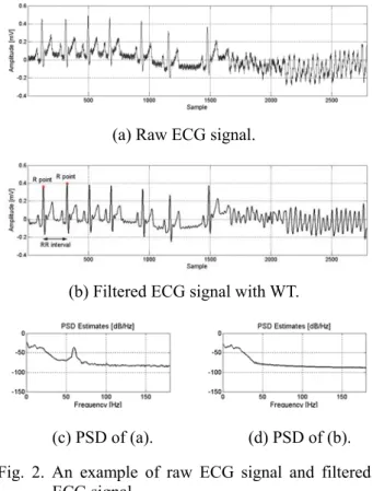
(a) Raw ECG signal.
(b) Filtered ECG signal with WT.
(c) PSD of (a). (d) PSD of (b). Fig. 2. An example of raw ECG signal and filtered
ECG signal. classification with even smaller learning data, we can
expect that the proposed algorithm, with relatively small learning data, would demonstrate better performance than other classifiers and be implemented faster on account of the reduction of feature dimensions. For a cross-validation procedure, this algorithm was compared with multilayer perceptrons (MLP) and fuzzy inference system (FIS) classifiers.
2. METHODS AND MATERIALS
2.1. Overview
The proposed algorithm includes preprocessing, feature extraction and feature dimension reduction by LDA and SVM based arrhythmia classification. Fig. 1 shows a block diagram of the proposed algorithm.
In this paper, the following arrhythmia categories have been considered: normal sinus rhythm (NSR), supraventricular tachycardia (SVT), arterial premature contraction (APC), ventricular tachycardia (VT), premature ventricular contraction (PVC) and ventricular fibrillation (VF).
For collecting arrhythmia data, we have used the ECG data from the MIT/BIH Arrhythmia Database digitized at a sampling rate of 360Hz. In addition, with the lack of VF data, Creighton University Ventricular Tachyarrhythmia Database and MIT-BIH Malignant Ventricular Arrhythmia Database, which had been sampled at 250 Hz, were resampled at 360 Hz and then used for VF.
The SVM classifier is the combination of NSR, APC, PVC, VF and other arrhythmia classifiers. The classification results of different classifiers form one output vector and the position of the highest value element of output vector indicates the membership with the appropriate class. Owing to the similar characteristics of the features of APC and SVT, their outputs of SVM are hardly distinguished. Opposed to APC, SVT is, however, inclined to occur in series. PVC and VT have much the same relationship. So, if output vector of said APC beat or PVC beat occurred more than three times consecutively, they were classified into SVT or VT respectively. Consequently, six types of arrhythmia were made to be classified by the proposed algorithm.
2.2. Preprocessing
Preprocessing is divided into noise cancellation,
QRS complex detection and beat segmentation for feature extraction and it cares about ECG signals sampled at 360 Hz. The wavelet transform (WT) has been verified as a good tool for preprocessing and QRS complex detection [8]. For the orthogonal wavelet transform, a discrete signal x(n) can be
expanded into the scaling function at j level as
follows;
( ) j[ ( )] j[ ( )]
x n =D x n +A x n , (1)
where Dj[x(n)] represents the detail signal at j level
and Aj[x(n)] represents the approximate signal at j
level. Here, j level signifies the decomposition at scale 2j. For noise cancellation such as baseline wander, 60 Hz interference and other high frequency noises, a filtered signal xf (n) is designed as
( ) [ ( )]- [ ( )]
f 2 8
x n =A x n A x n . (2)
The corresponding bandwidth of the filtered signal is 0.7Hz to 45Hz for 360 Hz sampling rate. In Fig. 2, an example of raw ECG signal and filtered ECG signal are presented and cancellation of unnecessary high and low frequency noises can be found in time domain (Fig. 2(b)) and in frequency domain (Fig. 2(d)).
For the detection of the QRS complex, the wavelet transform based method, proposed by Park et al. [9],
was used. For the filtered signal xf (n), the beat
segment was defined to begin at 200 msec (= 72
Preprocessing Noise cancellation with WT QRS complex detection Feature extraction F1, F2 from RR intervals F3~F17 from sub-band signals by WT Feature dimension reduction by LDA SVM arrhythmia classifier NSR APC PVC VF SVT VT <arrhythmia categories> Others Preprocessing Noise cancellation with WT QRS complex detection Feature extraction F1, F2 from RR intervals F3~F17 from sub-band signals by WT Feature dimension reduction by LDA SVM arrhythmia classifier NSR APC PVC VF SVT VT <arrhythmia categories> Others Fig. 1. Block diagram of proposed arrhythmia classifier.
sample points) before R peak and to end at 200 msec after R peak so that it could have a total length of 400 msec. All considered features were extracted from this beat segment.
2.3. Feature extraction
The arrhythmias classification by neural network classifier requires generation of the input vectors. Since a physician classifies arrhythmia with the information of rhythm and morphology, an input vector should include features that represent the rhythm and morphology properly. Therefore, in this
paper, the input vector fed to the classifier was determined to be composed of 2 features related to rhythm, and 15 features related to morphology. If we define that R(i) is the RR interval between present and just previous R peaks – an example is shown in Fig. 2(b), and K is a constant that corresponds to an RR interval that all men are generally expected to have, feature 1 and feature 2 can be calculated as
1 ( ) K Feature R i = (3) ) i ( R K Feature 1 + = 2 (4) considering the sampling rate of 360 Hz, 300 sample points are chosen as K. The mean and variance of feature 1 and feature 2, which were calculated for four different classes (NSR, APC/SVT, PVC/VT and VF), are presented in Fig. 3. For these statistics, arrhythmia beats of 10 records from the MIT/BIH arrhythmia database are used.
In the mean time, morphology related features should satisfy that the differences among the ECG waveforms are suppressed for the waveforms of the same type but are emphasized for the waveforms
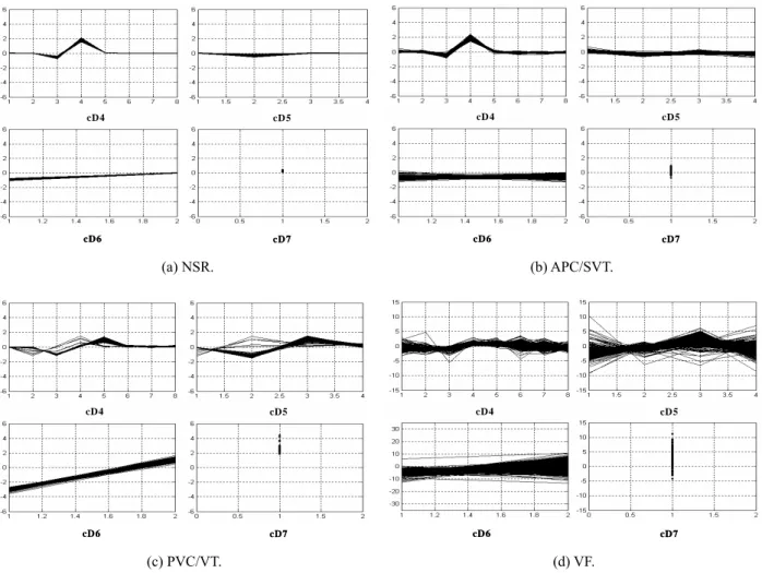
cD4 cD5 cD6 cD7 cD4 cD5 cD6 cD7 cD4 cD5 cD6 cD7 cD4 cD5 cD6 cD7 (a) NSR. (b) APC/SVT. cD4 cD5 cD6 cD7 cD4 cD5 cD6 cD7 cD4 cD5 cD6 cD7 cD4 cD5 cD6 cD7 (c) PVC/VT. (d) VF.
Fig. 4. The differences between detail coefficients’ distributions for different types of beats.
1.0025 1.486 1.4861 3.8396 0 1 2 3 4 5 6 NSR APC/SVT PVC/VT VF 1.0062 1.3293 0.7815 3.8354 0 1 2 3 4 5 6 NSR APC/SVT PVC/VT VF
(a) Feature 1. (b) Feature 2.
Fig. 3. The mean and variance of feature 1 and feature 2 for arrhythmia beats of 10 records from MIT/BIH arrhythmia database.
belonging to different types of beats. Because it is difficult to separate one from the other on the basis of only time or frequency representation, sub-band signals by wavelet transform were utilized for morphology features. For NSR and interested types of arrhythmia, their detail signals at levels 4, 5, 6 and 7 have representative components and obviously different distributions to each other. Level 4 signifies the decomposition at scale 24. Based on these facts, detail coefficients of these detail signals were chosen as features that could discriminate arrhythmia beats from the others. The differences between detail coefficients’ distributions for different types of beats can be found in Fig. 4. cD4 means that the detail coefficients at level 4 and the number of coefficients is 8. Similarly, cD5 at level 5, cD6 at level 6, cD7 at level 7 with the number of coefficients being 4, 2 and 1, respectively. These 15 coefficients were defined as feature 3 to feature 17.
2.4. Feature dimension reduction by LDA
Linear Discriminant Analysis (LDA) searches for those vectors in the underlying space that best discriminate among classes rather than those that best describe the data [10]. The goal of LDA is to seek a transformation matrix W that maximizes the ratio of the between-class scatter to the within-class scatter. Initially, we consider a within-class scatter matrix for the within-class scatter. A within-class scatter matrix Sw is defined as
(5)
where c is the number of classes, Ci is a set of data
belonging to the ith class, and mi is the mean of the ith class. The within-class scatter matrix represents the degree of scatter within classes as a summation of covariance matrices of all classes. Next, we consider a between-class scatter matrix for between-class scatter.
A between-class scatter matrix SB is defined as
(6)
where m is the mean of all classes. The between-class
scatter matrix represents the degree of scatter between classes as a covariance matrix of means of all classes. We seek a transformation matrix W that in some sense maximizes the ratio of the between-class scatter and the within-class scatter. The criterion function J(W) can be defined as ( ) . t B t w W S W J W W S W =
(7)
We can obtain the transformation matrix W as one that maximizes the criterion function J(W). Furthermore, given a number of independent features relative to which data is described, LDA creates a linear combination of these which yields the largest mean
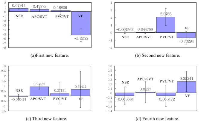
0.67914 0.47773 0.18806 -5.2255 -8 -7 -6 -5 -4 -3 -2 -1 0 1 2 NSR APC/SVT PVC/VT VF -0.007562 0.044768 2.0766 -0.70294 -2 -1 0 1 2 3 4 NSR APC/SVT PVC/VT VF
(a)First new feature. (b) Second new feature.
-0.040474 0.91487 0.27151 0.64412 -1.5 -1 -0.5 0 0.5 1 1.5 2 2.5 3 NSR APC/SVT PVC/VT VF -0.065684 0.0137 -0.065472 0.25241 -0.4 -0.3 -0.2 -0.1 0 0.1 0.2 0.3 0.4 0.5 0.6 NSR APC/SVT PVC/VT VF
(c) Third new feature. (d) Fourth new feature.
Fig. 5. Statistical characteristic of new features for arrhythmia beats of 10 records from MIT/BIH arrhythmia database for different classes.
∑∑
1 ∈ ) -)( -( c i x C t i i w i m x m x S = =∑
1 ) -)( -( c i t i i B m m m m S = = , ,differences of the desired classes [11]. As a result, if
there are c classes, the dimension of feature can be
reduced to c-1 extremely. Using fewer inputs to the
arrhythmia classifier, faster computation can be expected.
In this paper, assuming the number of classes is 5, the number of original features was designed to be reduced to 4 by LDA with guarantee of the comparable performance to that prior to reduction. The mean and variance of 4 features, which were newly generated by this process, are presented in Fig. 5. For different arrhythmia beats, their mean and variance are distributed in different ranges so that new features could also provide good tools for discrimination of arrhythmia beats.
2.5. SVM based arrhythmia classifier
The purpose of Support Vector classification is to devise a computationally efficient way of learning good separating hyperplanes in a high dimensional feature space. The SVM works in the high dimensional feature space formed by the nonlinear
mapping, φ(x) of the n-dimensional input vector into a
K-dimensional feature space. The equation of the hyperplane separating two different classes is given by the relation 0 1 (x) T ( ) K (x) 0 j j j y W ϕ X ω ϕ ω = = =
∑
+ = (8)with w=[ω0, ω1, ..., ωk]T is the weight vector of the network.
By introducing the so-called Lagrange multipliers, i
α the learning task of SVM is reduced to quadratic
programming. On account of these facts, there exist many highly effective learning algorithms [12-14], which result in the global minimum of the cost function and the best possible choice of the parameters of the neural network. And all operations in learning and testing are done using so-called kernel
functions. The kernel is defined as K(x,xi)=ϕ
x) ( ) x ( i ϕ ϕT .
In this paper, a radial basis function (RBF) was selected as the kernel and the parameters - kernel
width σ and margin-losses trade-off C, which
provided best classification, were fixed by experiments before learning. Simultaneously, the learning of SVM can be referred to as the separation of learning vectors xi into two classes of the destination values either di=1 or di=-1, with maximal separation margin. And this process is reduced to the
dual maximization problem of the function, Q( )α
defined as follows [12,15]:
(9)
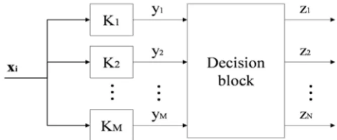
Fig. 6. The scheme of proposed SVM based classifier. with the constraints
(10)
where C is a user-defined trade-off constant as
previously mentioned and p is the number of learning
data pair (xi, di). C determines the balance between
the complexity of the network, characterized by the weight vector w and the error of classification of data.
The solution with respect to the Lagrange
multipliers gives the optimal weight vector Wopt, as
∑
==
NS i si sid
1 si opt(
x
)
w
α
ϕ
. The output signal y(x) ofthe SVM network is determined as the function of (11) kernels and the specific form of the nonlinear function need not be known. The positive value of y(x) is associated with membership of the particular class and the negative one with membership of the opposite class. Although SVM separates the data only into two classes, classification into additional classes is possible by applying either the “one against one” or: “one against all” method [16,17]. We designed a SVM based classifier as shown in Fig. 6.
The feature vectors xi fed to the neural classifier Ki and the outputs of each classifier form the vector
y=[y1, y2, ..., yM]T which signifies the potential of belonging to each class. Subsequently, with
user-defined rules, output values yj for some j may be
inhibited and additional output may be generated through a decision block. As a result, final outputs
z=[z1, z2, ..., zN]T are given. The position of the highest value element of z indicates the membership with the appropriate class.
3. RESULTS AND DISCUSSION
To evaluate the performance of the classifier, three measures are used and defined as:
(%) TP 100 Sensitivity TP FN = × + , (12)
x)
(
ϕ
) , x ( 2 1 -) (∑
∑∑
1 1 1 j i j i p i p j j i p i i dd K x Q = = = = α αα α∑
Ns 1 i 0x)
,
x
(
x)
(
=+
=
α
sid
iK
siω
y
∑
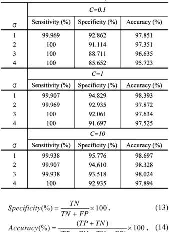
1 , 0 p i i id = = α 0≤ αi ≤C,Table 1. Comparisons of the classifier performance for different combination of parameters.
98.697 98.328 98.024 97.894 95.776 94.610 93.518 92.935 99.938 99.907 99.938 100 1 2 3 4 Accuracy (%) Specificity (%) Sensitivity (%) C=10 σ 98.393 97.872 97.634 97.525 94.829 92.935 92.061 91.697 99.907 99.969 100 100 1 2 3 4 Accuracy (%) Specificity (%) Sensitivity (%) C=1 σ 97.851 97.351 96.635 95.723 Accuracy (%) 92.862 91.114 88.711 85.652 Specificity (%) Sensitivity (%) 99.969 100 100 100 C=0.1 1 2 3 4 σ 98.697 98.328 98.024 97.894 95.776 94.610 93.518 92.935 99.938 99.907 99.938 100 1 2 3 4 Accuracy (%) Specificity (%) Sensitivity (%) C=10 σ 98.393 97.872 97.634 97.525 94.829 92.935 92.061 91.697 99.907 99.969 100 100 1 2 3 4 Accuracy (%) Specificity (%) Sensitivity (%) C=1 σ 97.851 97.351 96.635 95.723 Accuracy (%) 92.862 91.114 88.711 85.652 Specificity (%) Sensitivity (%) 99.969 100 100 100 C=0.1 1 2 3 4 σ (%) TN 100 Specificity TN FP = × + , (13) ( ) (%) 100 ( ) TP TN Accuracy TP FN TN FP + = × + + + , (14)
where TP stands for true positive, TN for true negative, FP for false positive and FN for false negative. When VF is concerned, TP represents VF being classified as VF and TN represents non-VF beat being classified as non-VF. Moreover, FP represents non-VF being classified as VF and FN represents VF being mis-classified as non-VF [6].
3.1. Parameter selection
SVM classifier parameters, with kernel width σ and
margin-losses trade-off C, affect the cost of learning
and the classification performance. We have selected optimal parameter values with trial experiments, in which the performance of the classifier was observed for the different combination of parameters. For these experiments, the goal of the classifier was confined to discriminate only NSR with 10 records from the MIT/BIH arrhythmia database. Table 1 presents the
performance of the classifier corresponding to each experiment. The performance is likely to get lower as
σ increases and the classifier has the better
performance with C=10 than with other Cs. So, we
chose the parameters - σ and C as 1 and 10
respectively.
3.2. Feature dimension reduction by LDA
Two of the most popular dimensionality reduction techniques are Principal Component Analysis (PCA) and Linear Discriminant Analysis (LDA). The former one deals with the data in its entirety for the principal component analysis without paying any particular attention to the underlying class structure, whereas the latter one deals with discrimination between classes. To certify the usefulness of LDA, the performance of the classifier was evaluated with original features, features reduced to 4 dimensions by PCA and features reduced to 4 dimensions by LDA. For this, 23 records from the MIT/BIH arrhythmia database, which contain NSR and other types of arrhythmias, were used and the interested classes were confined as NSR and others. For this task, the SVM classifier was used with different input features and Multilayer Perceptrons (MLP) and the Fuzzy Inference System (FIS) were additionally tried with them for cross-validation. The results of classification are summarized in Table 2. ORG indicates the results with the original 17 features, PCA with 4 features by PCA and LDA with 4 features by LDA.
For the SVM classifier, the overall performance of PCA seems to be lower than that of ORG by less than 1%. In the mean time, the overall performance of LDA shows to be higher than both that of PCA and that of ORG. Even though other classifiers were used, the reduced features by LDA indicated usefulness for classification. Consequently, we found that the dimension of features had been reduced effectively by LDA and the better performance could be obtained with a smaller number of features than that of original features. Furthermore, faster learning was possible due to lower dimensions of input features.
3.3. Performance of SVM arrhythmia classifier To verify the effectiveness of the SVM arrhythmia classifier, its performance was compared with that of well-known classifiers; Multilayer Perceptrons (MLP) Table 2. Comparisons of the classifier performance for different feature reduction methods (units, %).
98.249 99.659 95.415 99.674 Sensitivity PCA 92.587 92.652 91.465 93.645 Specificity 97.508 98.954 94.704 98.865 Accuracy 98.966 99.490 97.896 99.510 Sensitivity ORG 93.766 94.680 90.555 96.064 Specificity 98.116 98.704 96.901 98.742 Accuracy 98.964 95.166 99.633 Average 99.324 98.047 99.521 95.643 91.104 98.751 99.899 99.395 99.606 MLP FIS SVM Accuracy Specificity Sensitivity LDA 98.249 99.659 95.415 99.674 Sensitivity PCA 92.587 92.652 91.465 93.645 Specificity 97.508 98.954 94.704 98.865 Accuracy 98.966 99.490 97.896 99.510 Sensitivity ORG 93.766 94.680 90.555 96.064 Specificity 98.116 98.704 96.901 98.742 Accuracy 98.964 95.166 99.633 Average 99.324 98.047 99.521 95.643 91.104 98.751 99.899 99.395 99.606 MLP FIS SVM Accuracy Specificity Sensitivity LDA
and Fuzzy Inference System (FIS) classifiers.
For a MLP classifier, a three layer structure was used, including an input layer, a hidden layer and an output layer. Each input layer and output layer has 4 nodes and 5 nodes respectively. And, the hidden layer, using sigmoid functions as the membership functions, was made to have 10 nodes with best performance. The learning task was done by an error back propagation algorithm.
For a FIS classifier, input features were translated to linguistic values by the fuzzy inference, in which membership functions and fuzzy logic comprised of IF-THEN statements were used. A Gaussian curve was used for the membership functions, on which the performance of FIS is likely to be dependent, and its characteristic parameters were selected with repetitive experiments. A min-max method, also known as the Mandani inference method, was used for inference and a result was finally obtained by a gravity center defuzzification.
For the evaluation of each classifier, a total of 5630 beats were used and it consisted of 67438 NSR beats, 2318 APC and SVT beats, 8617 PVC and VT beats, 7175 VF beats and 82 other beats. All classifiers equally used 4 dimension features by LDA as input features. Table 3 shows the summarized results of cross-validation. The SVM classifier can discriminate NSR with accuracy of 99.307%, APC with 99.274%, SVT with 99.854%, PVC with 98.344%, VT with 99.441% and VF with 99.883%. The overall performance of the SVM classifier is generally better than that of the MLP classifier and that of the FIS classifier. And, the FIS classifier has the most inferior performance. This may be from the fact that the used features are not suitable for fuzzy inference and we could not find the best membership functions. For NSR and APC, the SVM classifier shows absolute superiority in all performance areas; sensitivity, specificity and accuracy. The sensitivity of the SVM classifier for NSR and VF is higher than that of the SVM classifier for other arrhythmias, for which MLP even demonstrate better sensitivity. And, the SVM classifier has mostly good specificity for all arrhythmias. The majority of errors are caused by
some arrhythmias not considered in this paper, such as LBBB (left bundle branch block), RBBB (right bundle branch block) and fusion beat. To obtain the above results, while the SVM classifier used 4135 beats in the learning task, the MLP classifier used 26512 beats, which is about six times more. Undoubtedly, when fewer beats were used for the MLP classifier, lower performances were obtained, but these are not shown here. Moreover, the CPU time taken to build the SVM classifier and MLP classifier were measured as 100.094 and 623.734 secs, respectively.
Finally, we can know that the proposed SVM classifier provides better performance than the MLP classifier with smaller learning data as well as than that of previous studies [1-6].
5. CONCLUSIONS
In this paper, we proposed a SVM based arrhythmia classification algorithm. Seventeen original input features were extracted from preprocessed signals by wavelet transform; 2 rhythm related features and 15 wavelet coefficient features. To improve the learning efficiency of the classifier, we attempted to reduce the original features to 4, the linear combination of original features, by LDA. Comparing the performance of the SVM classifier with different input features, the performance with features by LDA showed higher than with that by PCA and even with original features. So, we could see that LDA could reduce feature dimensions and act as a useful tool to improve the classifier performance at lower learning costs. To evaluate the SVM arrhythmia classifier, a cross-validation method was adopted. That is, the performance of it was compared with that of the MLP classifier and FIS classifier using dimension reduced features. The proposed SVM classifier showed satisfactory performances in discriminating six types of arrhythmia beats. The accuracy of discrimination of NSR, APC, SVT, PVC, VT and VF were 99.307%, 99.274%, 99.854%, 98.344%, 99.441% and 99.883%, respectively. The overall performance of the SVM classifier was comprehensively better than that of the Table 3. Comparisons of the performances with different classifiers (units, %).
99.350 99.121 92.396 98.975 98.049 89.623 98.651 98.123 92.2975 Average 99.307 99.274 99.854 98.344 99.441 99.883 96.215 99.951 100 98.937 99.632 99.993 99.657 88.294 82.821 92.157 91.695 99.751 98.572 98.374 99.148 98.377 99.444 99.934 89.296 100 100 99.362 99.636 100 99.623 80.574 81.345 89.754 87.188 99.254 98.276 98.374 99.148 97.505 98.701 99.903 92.021 100 100 97.9 98.859 99.958 98.984 85.185 84.706 93.085 92.484 99.341 NSR APC SVT PVC VT VF Accuracy Specificity Sensitivity Accuracy Specificity Sensitivity Accuracy Specificity Sensitivity SVM FIS MLP 99.350 99.121 92.396 98.975 98.049 89.623 98.651 98.123 92.2975 Average 99.307 99.274 99.854 98.344 99.441 99.883 96.215 99.951 100 98.937 99.632 99.993 99.657 88.294 82.821 92.157 91.695 99.751 98.572 98.374 99.148 98.377 99.444 99.934 89.296 100 100 99.362 99.636 100 99.623 80.574 81.345 89.754 87.188 99.254 98.276 98.374 99.148 97.505 98.701 99.903 92.021 100 100 97.9 98.859 99.958 98.984 85.185 84.706 93.085 92.484 99.341 NSR APC SVT PVC VT VF Accuracy Specificity Sensitivity Accuracy Specificity Sensitivity Accuracy Specificity Sensitivity SVM FIS MLP
MLP classifier and the FIS classifier. And, even with smaller learning data, the SVM classifier could provide better performance than the MLP classifier.
Furthermore, the proposed algorithm could be expected to offer faster implementation than other neural networks by the reduction of feature dimensions by LDA and by less-demanding learning data characteristics of the SVM classifier.
REFERENCES
[1] Y. H. Hu, S. Palreddy, and W. Tomkins, “A patient adaptable ECG beat classification using a
mixture of experts approach,” IEEE Trans.
Biomed. Eng., vol. 44, no. 9, pp. 891-900, September 1997.
[2] Y. H. Hu, W. Tomkins, J. L. Urrusti, and V. X. Alfonso, “Applications of artificial neural networks for ECG signal detection and
classification,” Electrocardiology, vol. 24, pp.
123-129, 1994.
[3] K. Minami, H. Nakajima, and T. Yoyoshima, “Real time discrimination of the ventricular tachyarrhythmia with Fourier-transform neural
network,” IEEE Trans. Biomed. Eng., vol. 46, no.
2, pp. 179-185, 1999.
[4] G. E. Oien, N. A. Bertelsen, T. Eftestol, and J. H. Husoy, “ECG rhythm classification using
artificial neural networks,” Proc. of the IEEE
Digital Signal Processing Workshop, pp. 514-517, 1996.
[5] T. Sugiura, H. Hirata, Y. Harada, and T. Kazui, “Automatic discrimination of arrhythmia
waveforms using fuzzy logic,” Proc. of the IEEE
Engineering in Medical and Biology Society, vol. 20, no. 1, pp. 108-111, 1998.
[6] L. Y. Shyu, Y. H. Wu, and W. Hu, “Using wavelet transform and fuzzy neural network for
VPC detection from the Holter ECG,” IEEE
Trans. Biomed. Eng., vol. 51, no. 7, pp. 1269-1273, 2004.
[7] R. Schalkoff, Pattern Recognition: Statistical,
Structural and Neural Approaches, Wiley, New York ,1992.
[8] S. Kadambe, R. Murray, and G. F. B. Bartels, “Wavelet transform-based QRS complex
detector,” IEEE Trans. Biomed. Eng., vol. 46, no.
7, pp. 838-848, July 1999.
[9] K. L. Park, K. J. Lee, and H. R. Yoon, “Application of a wavelet adaptive filter to
minimize distortion of the ST-segment,” Med.
And Biol. Eng. and Computing, vol. 36, no. 5, pp. 581-586, 1998.
[10] H. C. Kim, D. J. Kim, and S. Y. Bang, “Face
recognition using LDA mixture model,” Proc. of
the Pattern Recognition, vol. 2, pp. 925-928, 2002.
[11] A. M. Martinez and A. C. Kak, “PCA versus
LDA,” IEEE Trans. Pattern Analysis and
Machine Intelligence, vol. 23, no. 2, pp. 228-233, 2001.
[12] A. Smola and B. Scholkopf, “A tutorial on
support vector regression,” NeuroColt Tech. Rep.
NV2-TR-1998-030, Royal Holloway College, Univ. London, London, U. K., 1998.
[13] O. L. Mangasarian, “Lagrangian support vector
machines,” J. Machine Learning Res., vol. 1, pp.
161-177, 2001.
[14] J. Platt, “Fast training of SVM using sequential
optimization,” Advances in Kernel
Methods-Support Vector Learning, B. Scholkpf, C. Burges, and A. Smola, Eds. Cambridge, MIT Press, U.K., pp. 185-208, 1998.
[15] C. Burges, “A tutorial on support vector
machines for pattern recognition,” Knowledge
Discovery and Data Mining, U. Fayyad, Ed. Norwell, Kluwer, MA, pp. 1-43, 2000.
[16] K. Crammer and Y. Singer, “On the learn ability and design of output codes for multi-class
problems,” Proc. 13th Conf. Computational
Learning Theory, pp. 35-46, 2000.
[17] C. W. Hsu and C. J. Lin, A Comparison of
Methods for Mmulti-class Support Vector Machines, Nat. Taiwan Univ., Taiwan, 2000.
Mi Hye Song received the B.S. and
M.S. degrees in Engineering from Yonsei University, Korea, in 2003, and 2005, respectively. Since 2005, she has been a Ph.D. student in the Biomedical Engineering Department at Yonsei University. Her research interests include ECG signal processing, digital signal processing, real-time system design, and medical instrumentation.
Jeon Lee received the B.S. and M.S.
degrees in Engineering from Yonsei University, Korea, in 1996, and 1999, respectively. Since 1999, he has been a Ph.D. student in the Biomedical Engineering Department at Yonsei University. In 2005, he was awarded the Young Investigator Award at APCMBE05 sponsored by IFMBE. His research interests include nonlinear bio-signal processing, bio-impedance applications, mathematical modeling of cardiovascular circulation, measurement systems with wearable sensors, and others.
Sung Pil Cho received the B.S. and
M.S. degrees in Engineering from Yonsei University, Korea, in 2001, and 2003, respectively. Since 2004, he has been a Ph.D. student in the Biomedical Engineering Department at Yonsei University. His research interests include biomedical signal processing, adaptive filter theory, and sleep disorders.
Kyoung Joung Lee received the B.S.,
M.S., and Ph.D. degrees in Electrical Engineering from Yonsei University, Seoul, Korea, in 1981, 1983, and 1988, respectively. Since 1982, he has worked in Biomedical Engineering at Yonsei University. He was a Visiting Professor at Case Western Reserve University, Ohio, U.S.A. in 1993. He is currently a Biomedical Engineering Professor at Yonsei University. His research interests include signal processing, cardiovascular modeling, cardiac diagnosis, and medical instrumentation.
Sun Kook Yoo received the B.S., M.S.,
and Ph.D. degrees in Electrical Engineering from Yonsei University, Seoul, Korea, in 1981, 1985, and 1989, respectively. He was an Assistant Professor of Electrical Engineering at Soonchunhyung University, from 1990 to 1994, and a Visiting Associate at the Department of Radiology, University of Iowa, Iowa City, from 1998 to 2000. Currently, he is an Associate Professor in Medical Engineering, Yonsei University, and a Director of the Center for Emergency Medical Informatics (CEMI). His research interests include 3-D visualization, telemedicine, and real-time system design.