Algorithms for Integrated Computer-Based Analyses
of Big Environmental Databases
Dissertation
der Mathematisch-Naturwissenschaftlichen Fakultät der Eberhard Karls Universität Tübingen
zur Erlangung des Grades eines Doktors der Naturwissenschaften
(Dr. rer. nat.)
vorgelegt von M.Sc. Abduljabbar Asadi
Geboren am 04. 04. 1985, in Sanandaj, Iran
Tübingen 2017
Tag der mündlichen Qualifikation: 25 Sept 2107
Dekan: Prof. Dr. Wolfgang Rosenstiel
1. Berichterstatter: Prof. Dr. Peter Dietrich 2. Berichterstatter: Prof. Dr. Erwin Appel
life, and because of the understanding and knowledge which gives me I am able to solve all challenges in my life.
I dedicate this work to my dear wife; Soniya Hatami who has tolerated hardship and encouraged me all the way and whose encouragement has made sure that I give it all it takes to finish which I have started. You were the most important reason for this success. I am truly thankful for having you in my life. I love you so much. I also dedicated this work to the childhood memories of my son; Ermiya, because he spent his childhood with me during doing this thesis, I promise that I have enough time for you now.
I dedicated this work to the endured hands of my father Taofigh and my mama Khanoom, who are waiting for me and always loved me unconditionally. Thank you so much, I love you unconditionally, and will never forget you. I would like to extend my thanks to my father-in-law Eskandar and mother-in-law Golbakhi; for their encouragement and involvement in my efforts, and for their love. Thank you so much.
I would like to express my deepest gratitude to my supervisor Professors Peter Dieterich and my project supervisor Dr. Hendrik Paasche for their unwavering support, collegiality, and mentorship throughout this project.
i
Knowledge of the spatial distribution of geotechnical, hydrological, petroleum, and environmental parameters in the subsurface is essential in environmental earth sciences. Latest developments in engineering geophysics and remote sensing data acquisition provide a large set of techniques for non-invasive and in situ data recording for high-resolution ground probing. We developed different strategies based on knowledge discovery for analyzing environmental earth science databases. One important type of these databases is geophysical tomography, which offers 2D or 3D valuable and unique information about the internal composition of the ground. Based on different data mining and machine learning (i.e., feature extraction, Artificial Neural Networks, etc.) techniques we developed a data analysis strategy based on artificial neural networks (ANNs) allowing for 2D or 3D probabilistic prediction of sparsely measured earth properties constrained by geophysical tomography fully accounting for tomographic reconstruction ambiguity. Furthermore, we try to take the uncertainty or variability of the input data into account for proving the results of this method. Additionally, we have evaluated whether the training performance of the prediction model of ANNs can be used to rank geophysical tomograms. Such prediction model can contribute to solving hydrological, petroleum, or engineering exploration tasks in a data-driven manner. Another important issue is mapping the earth which is a fundamental prerequisite required to address various environmental and economic issues, such as mining target identification, soil conservation, or ecosystem management. The datasets for mapping are either technical or subjective. We show the first attempts towards integrating technical and subjective spatial datasets in an automated and rapid manner based on different data mining algorithms (i.e., graph analysis, boundary detection, clustering, etc.). Such method aims to produce a crisp or fuzzy classified map outlining dominant structures in the database optimally consistent with all available information.
ii
Einsicht in die räumliche Verteilung geotechnischer und hydrologischer Untergrundeigenschaften sowie von Reservoir- und Umweltparametern sind grundlegend für geowissenschaftliche Forschungen. Entwicklungen in den Bereichen geophysikalische Erkundung sowie Fernerkundung resultieren in der Verfügbarkeit verschiedenster Verfahren für die nichtinvasive, räumlich kontinuierliche Datenerfassung im Rahmen hochauflösender Messverfahren. In dieser Arbeit habe ich verschiedene Verfahren für die Analyse erdwissenschaftlicher Datenbasen entwickelt auf der Basis von Wissenserschließungsverfahren. Eine wichtige Datenbasis stellt geophysikalische Tomographie dar, die als einziges geowissenschaftliches Erkundungsverfahren 2D und 3D Abbilder des Untergrunds liefern kann. Mittels unterschiedlicher Verfahren aus den Bereichen intelligente Datenanalyse und maschinelles Lernen (z.B. Merkmalsextraktion, künstliche neuronale Netzwerke, etc.) habe ich ein Verfahren zur Datenanalyse mittels künstlicher neuronaler Netzwerke entwickelt, das die räumlich kontinuierliche 2D oder 3D Vorhersage von lediglich an wenigen Punkten gemessenen Untergrundeigenschaften im Rahmen von Wahrscheinlichkeitsaussagen ermöglicht. Das Vorhersageverfahren basiert auf geophysikalischer Tomographie und berücksichtigt die Mehrdeutigkeit der tomographischen Bildgebung. Außerdem wird auch die Messunsicherheit bei der Erfassung der Untergrundeigenschaften an wenigen Punkten in der Vorhersage berücksichtigt. Des Weiteren habe ich untersucht, ob aus den Trainingsergebnissen künstlicher neuronaler Netzwerke bei der Vorhersage auch Aussagen über die Realitätsnähe mathematisch gleichwertiger Lösungen der geophysikalischen tomographischen Bildgebung abgeleitet werden können. Vorhersageverfahren wie das von mir vorgeschlagene, können maßgeblich zur verbesserten Lösung hydrologischer und geotechnischer Fragestellungen beitragen.
ii
ökologischer Fragestellungen ist, wie z.B., die Identifizierung von Lagerstätten, den Schutz von Böden, oder Ökosystemmanagement. Kartierungsdaten resultieren entweder aus technischen (objektiven) Messungen oder visuellen (subjektiven) Untersuchungen durch erfahrene Experten. Im Rahmen dieser Arbeit zeige ich erste Entwicklungen hin zu einer automatisierten und schnellen Integration technischer und visueller (subjektiver) Daten auf der Basis unterschiedlicher intelligenter Datenanalyseverfahren (z.B., Graphenanalyse, automatische Konturerfassung, Clusteranalyse, etc.). Mit solchem Verfahren sollen hart oder weich klassifizierte Karten erstellt werden, die das Untersuchungsgebiet optimal segmentieren um höchstmögliche Konformität mit allen verfügbaren Daten zu erzielen.
vi
Abstract ... i
Zusammenfassung ... ii
Contents ... vi
List of Figures ... xii
List of Tables ...xiii
List of Symbols ... xiv
List of Abbreviations ... xv
Chapter 1 Introduction ... 1
1.1 Knowledge Discovery in Databases (KDD) ... 1
1.2 Uncertainty and Error in Data ... 5
1.3 Subjective and Technical Data ... 7
1.4 Human in the Loop (HTL) ... 8
1.5 KDD in Earth Sicences ... 11
1.6 Objectives of This Thesis ... 12
Chapter 2 2D Probabilistic Prediction of Sparsely Measured Earth Properties Constrained by Geophysical Imaging Fully Accounting for Tomographic Reconstruction Ambiguity ... 15
2.1 Abstract ... 15
2.2 Introduction ... 17
2.3 Methodology ... 20
2.3.1 Geophysical Tomography as Feature Construction Problem ... 20
2.3.2 Feature Selection by Prediction ... 22
2.3.3 Processing Flow ... 24
2.4 Case Study ... 26
2.4.1 Tomographic Data Simulation... 26
2.4.2 Feature Construction By Tomographic Reconstruction ... 28
2.4.3 Generation of Sparse Exploration Target Parameters ... 31
2.4.4 Setting up the Artificial Neural Network ... 32
2.5 Results and Discussion ... 34
vii
2.5.2 Ranking of Tomograms ... 38
2.6 Conclusions ... 41
Chapter 3 Spatially Continuous Probabilistic Prediction of Sparsely Measured Ground Properties Constrained by ill-posed Tomographic Imaging Considering Data Uncertainty and Resolution ... 43
3.1 Abstract ... 43
3.2 Introduction ... 45
3.3 Methodology ... 48
3.3.1 Artificial Neural Networks (ANNs) ... 48
3.4 Processing Flow ... 51
3.5 The Database ... 52
3.5.1 The Field Site ... 52
3.6 Data Acquisition ... 53
3.6.1 Tomography ... 53
3.6.2 Sparse Logging Data ... 54
3.7 Processing ... 55
3.7.1 Tomography ... 55
3.7.2 Tomographic Uncertainty ... 57
3.7.3 Logging Data Uncertainty ... 58
3.8 Setting up the ANNs ... 59
3.8.1 Combination of Tomograms for ANNs ... 59
3.8.2 Training Without Error Incorporation ... 60
3.8.3 Training With Error Incorporation ... 60
3.8.4 Training With Separate Logging Data ... 61
3.8.5 Training Accounting for Resolution Difference ... 61
3.8.6 Selecting the Number of Neurons in the Hidden Layer ... 62
3.9 Results and Discussion ... 63
3.9.1 Prediction Results of ANNs ... 63
3.9.2 Training Without Error Incorporation ... 63
3.9.3 Training With Error Incorporation ... 64
3.9.4 Training With Separate Logging Data ... 66
3.9.5 Taking Resolution Differences into Account ... 67
viii
3.9.7 Transferability and Outreach of Results ... 69
3.10 Conclusions ... 70
Chapter 4 Conceptual Developments for Clustering Mapped Data Emanating From Technical Sensors and Subjective Insights of Human Experts ... 72
4.1 Abstract ... 72
4.2 Introduction ... 74
4.3 Methodology ... 76
4.3.1 The K-means Clustering ... 76
4.3.2 Graph Theory and Shortest Path ... 78
4.3.3 Boundary Detection ... 78
4.3.4 Sampling Strategy ... 80
4.3.5 Processing Flow ... 81
4.4 The Datasets... 85
4.4.1 The Synthetic Datasets ... 85
4.4.2 The Field Datasets ... 86
4.5 Experiments and Results ... 88
4.5.1 Application to the Synthetic Dataset ... 88
4.5.2 Application to the Field Dataset ... 91
4.6 Conclusions ... 96
Chapter 5 Summary and outlook ... 97
5.1 Data Mining Techniques Add Value to Geophysical Tomography and Logging Data ... 97
5.1.1 Taking Data Uncertainty into Account in the Machine Learning Prediction Part ... 99
5.1.2 Choosing Optimum Parameters for Artificial Neural Networks ... 100
5.1.3 Testing with Different Tomograms and Target Parameters ... 101
5.2 Human in the Loop for Mapping, Integration, and Segmentation of Geophysical Datasets .... 102
5.2.1 Further Testing the Idea of the Human in the Loop for Integration and Segmentation of Geoscientific Datasets ... 103
References ... 105
Appendix A Towards Probabilistic Prediction of Soil Moisture in the Schäfertal Catchment ... 113
A.1 Introduction ... 113
A.2. Methodology ... 113
ix
A.4 Conclusion... 116
Appendix B A New Methodology for Prediction of 2D Distributions of Sparsely Measured Logging Data under Full Consideration of Tomographic Model Generation Ambiguity ... 118
B.1 Abstract ... 118
B.2 Introduction ... 118
B.3 Artificial Neural Networks (ANN) ... 119
B.4 Methodology... 120
B.5 Application to a Field Dataset ... 123
B.6 Conclusions ... 124
Appendix C 2D probabilistic prediction of sparsely measured geotechnical parameters constrained by tomographic ambiguity and measurements errors ... 125
C.1 Abstract ... 125
C.2 Introduction ... 125
C.3 Artificial Neural Networks (ANN) ... 127
C.4 The Processing Flow ... 128
C.5 Results ... 129
C.6 Conclusions ... 131
Appendix D Predicting Porosity According to Ensembles of Collocated Radar and Seismic Tomographic Models with Artificial Neural Networks ... 132
D.1 Abstract ... 132
Appendix E Conceptual Developments for Clustering Mapped Data Emanating from Technical Sensors and Subjective Insights of Human Experts ... 134
E.1 Abstract ... 134
Appendix F Probabilistic Integration of Tomograms and Logging Data Accounting for Tomographic Ambiguity and Logging Data Errors ... 136
F.1 Abstract ... 136
Appendix G Incorporating Hyperspectral Datasets in the Integration Strategy Introduced in Chapter 4 138 G.1 Process ... 138
Appendix H Histogram Normalization ... 142
H. 1 Process and Results ... 142
xii
Figure 1-1: The structure of knowledge discovery in databases (KDD). It is based on the three important steps: preprocessing, data mining, and information evaluation by the end user. During these three steps the effective information will be extracted from big data bases by KDD. ... 3 Figure 1-2: Four combinations of accuracy and precision (Haibo, 2014).. ... 7 Figure 1-3: Four different interactions between KDD and humans. (a), (b), (c), and (d) show
unsupervised, supervised, semi-supervised, and human in the loop approaches, respectively (Holzinger, 2016)... ...10 Figure 2-1: Schematic sketch of a geophysical cross-borehole tomographic experiment with
sources and receivers in the left and right boreholes...21 Figure 2-2: Flowchart of the processing workflow for probabilistic prediction of spatially
continuous models of sparsely measured target parameters and ranking non-sparse tomograms achieved from inversion or feature construction algorithms... ...25 Figure 2-3: Original synthetic models representing ground truth. (a) Layered ground assumed.
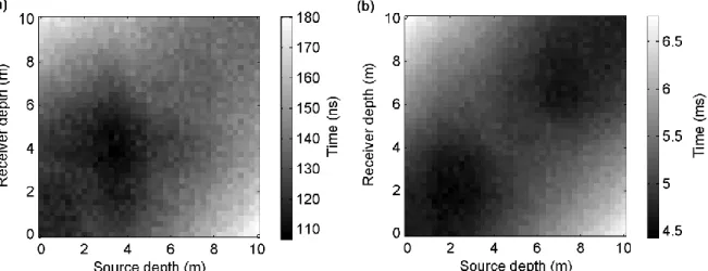
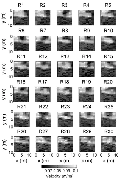
(b) Porosity variability in the ground. (c) Radar velocity and (d) seismic velocity are obtained from traditional deterministic petrophysical transfer functions used to convert porosity into physical parameters. (e) and (f) scatter plots of the models given in (b) and (c), and (b) and (d), respectively... ...27 Figure 2-4: Traveltimes of the (a) radar and (b) seismic tomographic datasets... ...29 Figure 2-5: 30 tomographic reconstructions of radar wave propagation velocity distributions
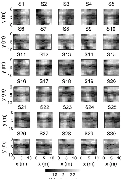
achieved by fully non-linear self-organizing inversion (Paasche, 2015). The 30 tomograms are achieved by independent inversion runs and fit the underling tomographic dataset equally well.. ...30 Figure 2-6: The same as in Figure 2-5 but for the seismic tomograms... ...31 Figure 2-7: Sparse porosity borehole logging data acquired in the boreholes at the (a) left (x=0
m) and (b) right (x=10 m) model edges (see Figure 2-3). Original porosity represents the true information of the ground. Logging porosity represents the modelled response of a realistic borehole porosity logging probe... ...32 Figure 2-8: MSE from ANN training for all combinations of spatially continuous tomograms. (a)-(e) represent the results of using ANNs with 3,5,10,20 and 50 neurons, respectively...34 Figure 2-9: Regression results of the training procedure of the ANN when using R30 and S30
tomograms as input and the (a) original porosity (RSOP) and (b) logging porosity (RSLP) as output information. Note, only the radar and seismic velocity information of the left and right model edges has been used for training...34 Figure 2-10: Prediction results of spatially continuous 2D porosity models based on the sparse
xiii
Relative frequency of porosity prediction from ANN models trained with original porosity. (b) The same as (a) but overlain by minimum and maximum range of true porosity of the ground (see Figure 2-3) shown by dashed black lines. (c) and (d) are analogue to (a) and (b) but for logging porosity instead of original porosity. Predicted porosities outside the displayed range are accumulated at the bins with lowest and highest porosities. They correspond to the ANN models trained with remaining high MSE... ...36 Figure 2-11: Ranking of tomograms (Figure 2-5 and 2-6) according to their relationships with
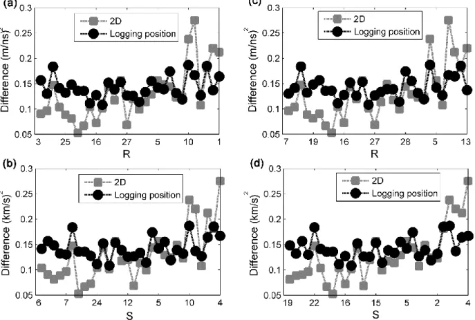
reality. RSOP rank radar and seismic models according to their combination with original porosity for training the ANN models. Likewise RSLP rank radar and seismic velocity tomograms according to their combination with logging porosity for training the ANN models. This ranking has been outcome from ANN with three neurons in the hidden layer. .. ...38 Figure 2-12: Summed squared differences of 30 tomographic radar (R) and seismic (S) velocity
tomograms from the true radar and seismic velocity models (Figures 2-3c, and 2-3d). The ordering of the model number (abscissa) corresponds to those proposed by the ANNs trained with three neurons in the hidden layer (Figure 2-11). The black circles illustrate differences at the left and right edges (logging positions) of the tomograms. The gray rectangles illustrate the difference of the entire 2D area. (a) and (b) correspond to the ANN trained with original porosity. (c) and (d) correspond to the ANN trained with logging porosity.. ...39 Figure 3-1: Structure of artificial neural networks (ANNs). ANNs are consisting of three
interconnected layers. The input layer prepares data for feeding the ANN. The operation of hidden layer is based on sets of input information, weights of inputs w and bias parameter b. Neurons in this layer form a feedforward network with sigmoid formation. The operation of the output layer has been determined by the hidden layer and is connected to the results of the ANN training step... ...48 Figure 3-2: Processing workflow to probabilistically predicting spatially continuous models for
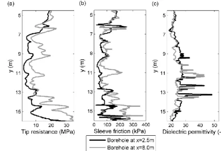
sparsely measured target parameters and geophysical tomograms achieved from fully non-linear inversion. Based on the training strategy, v determines the number of prediction models resulted from ANNs... ...51 Figure 3-3: Target parameter logging data acquired by direct push technology at x=2.75 m and
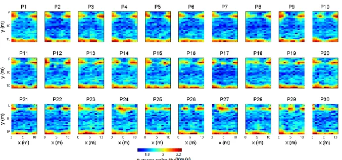
x=8.0 m for (a) tip resistance, (b) sleeve friction, and (c) dielectric permittivity.. ...54 Figure 3-4: 30 tomographic reconstructions of radar-wave propagation velocity achieved by fully
non-linear (global-search) inversion. The 30 tomograms are achieved by independent inversion runs and fit the underling tomographic dataset equally well... ...55 Figure 3- 5: The same as in Figure 3- 4 but for P-wave velocity... ...56 Figure 3- 6: The same as in Figure 3- 4 but for S-wave velocity... ...57 Figure 3-7: Tip resistance error calculation based on a low pass zero-phase digital filter. The
black line in Figure 3-7a determines the measured tip resistance; the gray line shows the filtered log. In Figure 3-7b the relative difference between measured and filtered tip resistance are shown which is considered as data noise component. Figure 3-7c determines the slope based on the low pass zero-phase digital filter in Figure 3-7a. .. ...59
xiv
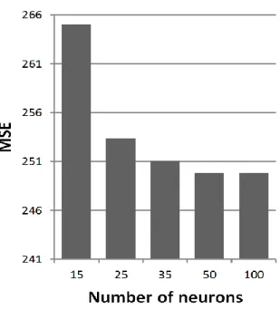
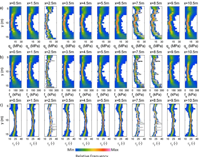
Figure 3-8: MSE from ANN training for all combinations of spatially continuous tomograms with 15, 25, 35, 50, and 100 neurons in the hidden layer. Based on this comparison 50 neurons have been selected as optimal number of neurons.. ...62 Figure 3-9: Prediction results of spatially continuous 2D target parameters based on the sparse
logging data and 27,000 combinations of spatially continuous tomograms (Figure 3-4, 3-5 and 3-6) shown as histographic plot. 2D probabilistic prediction plots show (a) tip resistance, (b) sleeve friction, and (c) dielectric permittivity prediction. The dotted white lines show the measured logging data of target parameters (Figure 3) that are used for training the ANN. Red colors correspond to high relative frequencies. Blue colors correspond to low relative frequencies... ...64 Figure 3-10: The same as in Figure 3-9, but trained considering tomographic and logging
uncertainty when training the ANN... ...65 Figure 3-11: The same as in Figure 3-10, but now training was individually performed for logs at
x =2.75 m and x = 8.0 m.. ...66 Figure 3 -12: The same as in Figure 3- 11 but, now repeatedly considering individual samples
from the logging datasets per grid cell when training the ANN, rather than averaging over all samples corresponding to a grid cell... ...67 Figure 3-13: Example of comparison of tip resistance predictions at x= 6.5m drawn from Figures
3-9, 3-10, 3-11, and 3-12. Trained (a) without error incorporation, (b) with error incorporation, (c) separate logging data, and (d) accounting for resolution difference between logs and tomograms.. ...69 Figure 4-1: Different types of boundaries in an image (a) step (b) line (c) ramp (d) roof... ...79 Figure 4-2: Processing workflow to integration and segmentation of subjective and objective
datasets. After normalizing the datasets two processing branches will be followed in the workflow. In the right part the similarity only based on the objective data will be calculated. Simultaneously in the left part the boundary of the subjective and objective maps will be extracted. Then, the new information vector based on results of these two branches will be calculated. This new information vector will be considered as new dataset and will be the input for the clustering algorithm. . ...82 Figure 4-3: Synthetic datasets for a 30*30 2D domain with (a) subjective map, (b) and (c)
objective technical maps. The subjective map shows structures mostly the same as in the technical maps, but with step boundaries and noise free. The technical maps show structures with different boundaries (i.e., step, line, roof, and ramp), noise, and anomalies from anthropogenic effects.. ...85 Figure 4-4: Two subjective maps of the Schäfertal catchment created by (a) (Borchardt 1985;
Ollesch et al. 2005) and (b) Landesamt für Geologie und Bergwesen Sachsen-Anhalt. They show the structures in this catchments based on observations recorded by scientists... ....86 Figure 4-5: Four attributes shown as objective or technical maps; (a) elevation, (b) slope, (c)
SAGA wetness index, and (d) annual potential incoming solar radiation derived form a 2-m digital elevation model for the Schäfertal catchment (Schröter et al., 2015). ...87
xv
Figure 4-6: 900*900 Gaussian similarity matrix for the data points in the synthetic dataset based on the absolute values in technical maps. The similarity of points is a value between 0 and 1.. ...88 Figure 4-7: Boundary information for the maps in the synthetic datasets. (a) Extracted boundaries
based on Canny boundary detection for the subjective map, (b) and (c) extracted boundaries based on the χ2 distances for technical maps, (d) calculated total boundary map of subjective and objective boundary maps... ...89 Figure 4-8: 900*900 matrices resultant from Dijkstra algorithm (a) all shortest paths and (b) all
path lengths for data points in the synthetic dataset... ...90 Figure 4-9: 900*900 matrix as new information vector resultant from similarity, shortest paths,
and path lengths matrices. The columns show 900 samples or data points and rows show 900 attributes or variable layers. This matrix carries the information about colors and boundary information of points in the map... ...90 Figure 4-10: means clustering results for the synthetic dataset with two strategies. (a) The k-means clustering results based on the new information vector resultant from the introduced strategy in this chapter, (b) the results of clustering without considering the boundary information of the subjective map. 6 cluster are desired in this dataset... ...91 Figure 4-11: Boundary information extracted from subjective maps in the Schäfertal catchment.
(a) Canny’s boundary detection results for the subjective map shown in Figure 4-4a. Problems with corners and junctions exist (see inlet), (b) and (c) Gaussian filtering for extracting bulky boundary subjective maps showed in Figure 4-4a and 4b, respectively... .92 Figure 4-12: Boundary information for (a) TWI and (b) insolation maps of the Schäfertal
catchment based on the χ2 distance. (c) Presents the total boundary map of subjective and objective maps for the Schäfertal catchment. ...93 Figure 4-13: (a) The selected s=1000 sampling points using systematic sampling selection
strategy. (b) The shortest path and (c) path length resultant from Dijkstra algorithm for the exemplary point selected at x=640.2 and y=5725 km to all other points in the map... ...94 Figure 4-14: The results of clustering the maps of the Schäfertal catchment with two strategies,(a)
the k-means clustering results on the new information vector resultant from the introduced strategy in this chapter, (b) presents the results of clustering without considering the boundary information (Schröter et al., 2015). 30 clusters are desired in this catchment, each color determine an independent cluster. ...95 Figure 4-15: The same as in Figure 4-14a, but now with sampling size reduced to (a) 500 and
(b) 250 samples.. ...95 Figure A-1: Land use map created by Schröter et al., (2015). Arable land is depicted by light gray,
grassland by dark gray colors... ... 114 Figure A-2: Four topographic attributes as objective or technical maps; (a) elevation, (b) slope,
(c) SAGA wetness index, and (d) annual potential incoming solar radiation derived form a 2-m digital elevation 2-model for the Schäfertal catch2-ment (Schröter et al., 2015). ... 114
xvi
Figure A-3: Soil moisture measurements in the Schäfertal. Locations for sampling the target parameter volumetric soil moisture are indicated by black dots... ... 115 Figure A-4: An exemplary result of regression in the training phase (a and b) and the test phase
(c and d) in crop (a and c) and grass (b and d) area.. ... 116 Figure A-5: (a) Probabilistic map of volumetric soil moisture content using ANN models based on
the grass and crop land use. The scale for each point is 50*50 m. Each glyph depicts soil moisture (color) and relative frequency (length). One exemplary glyph is zoomed in Figure A-5a to present the results of the 1000 ANN models for the related position. (b) shows the most likely soil moisture extracted from (a)... ... 117 Figure B-1: Structure of an Artificial Neural Network. We have three layers. The input layer
prepares data for feeding the ANN. The operation of the hidden layer is determined by inputs and weights of inputs (W). The operation of the output layer is guided by the hidden layer and connected to the results of ANN training.. ... 120 Figure B-2: Flowchart of processing steps for the prediction of 2D tip resistance models and
tomographic model ranking.. ... 121 Figure B-3: Geophysical velocity tomograms achieved by fully non-linear SOI. Rectangular grid
cells of 1 m lateral and 0.5 m vertical side lengths have been used for model parameterization. The black lines illustrate (a) 30 radar, (b) 30 S-wave, (c) 30 P-wave velocity models... ... 122 Figure B-4: Results of our 2D tip resistance prediction shown as histographic plot. The dotted
white lines show the measured logging data of tip resistance that are used for training the ANN. Red colors correspond to high relative frequencies. Blue colors correspond to low relative frequencies. Note the reduced sharpness of prediction at depths where the logging data are different and cannot be brought in full compliance with the velocity variations in the tomograms. ... 123 Figure B-5: MSE from ANN training for 30 models of radar, S-wave and P-wave velocity. Blue
color for radar models, black color for S-wave and red color for P-wave seismic models. Models with low MSE can be brought more easily in compliance with the tip resistance logging data. .. ... 124 Figure C-1: Structure of a three-layer Artificial Neural Network. The input layer prepares data for
feeding the ANN. The operation of the hidden layer is determined by inputs and weights of inputs (W). The operation of the output layer is guided by the hidden layer and connected to the results of ANN training.. ... 127 Figure C-2: Processing steps for the prediction of 2D sleeve friction models constrained by ill-posed geophysical tomography.. ... 128 Figure C-3: 2D geophysical velocity tomograms illustrated as laterally neighboured 1D velocity
panels. The black lines illustrate 30 equivalent (a) radar, (b) P-wave, (c) S-wave velocity models. Tomographic grid cells have 0.5 m and 1m vertical and lateral side lengths, respectively. ... 130
xvii
Figure C-4: Results of our 2D probabilistic prediction of sleeve friction. The dotted black lines show the measured logging data of sleeve friction that are used for training the ANN and calculation of the logging error. Red color corresponds to high relative frequencies. Blue color corresponds to low relative frequencies. Note that the ANNs trained with (a) with the MSE performance measure offer increased ranges of sleeve friction compared to the results (b) achieved when using the WMSE... ... 131 Figure G-1: Two exemplary bands of the hyperspectral data, each band carries random noise
and anthropogenic effects... ... 138 Figure G-2: (a) 72 bands of information for one pixel in 2D area, red, gray, and blue line show
measured data, fitted linear model, and difference between measured data and fitted model, respectively. (b) all measured data (red line) and difference between measured data and fitted liner model for 10000 pixel in the 2D area. The selected two position presents the decreasing of the difference between noisy points (lower bands) and normal points (higher bands), in the measured data and fitted data, which in fitted results this difference has been decreased. ... 138 Figure G-3: Results of the clustering method. (a) Total boundary map of selected 72 bands, (b)
Clustering results for small part of Schäfertal (100*100 pixel) based on the hyperspectral datasets for desired four clusters... ... 139 Figure H-1: Histogram normalization for (a) elevation, (b) slope, (c) TWI, and (d) insolation maps
of the Schäfertal catchment... 141 Figure H-2: Boundary detection results. (a) Boundary of TWI, (b) boundary of insolation, (c) total
boundary of technical maps, and (d) total boundary of subjective and technical maps... .. 142 Figure H-3: (a) Distribution of 1000 samples. (b) - (d) clustering results for 30 clusters based on
xiii
Table 2-1: Parameters used in equations 4-1,4-2, and 4-3. All layers A-G are considered to consist of sandy or gravelly saturated sediments; Layers A and B are considered slightly consolidated, the pore fluid in layers D and G comprises a non-aqueous phase liquid component in addition to water. ...28
xiv Symbol Denotation
𝑎 Coefficient
Σ Relative noise component (coefficient)
C Velocity of an electromagnetic wave in air
εf Relative dielectrical permittivity of dry matrix material
εm Relative dielectric permittivity of dry matrix material
εr Dielectric permittivity
Ε Dielelctrical permittivity/ weights of the related training tuples
fs Sleeve friction
qc Tip resistance
I / i Coefficient
J / j Coefficient
N Number of tuples
P∆ Uncertainty of P-wave velocity tomogram
R∆ Uncertainty of radar-wave velocity tomogram
S∆ Uncertainty of S-wave velocity tomogram
Ρ First absolute derivative between related neighboured readings in the log
Pd Value of data point p in a d-dimensions dataset
Θ Angle
Φ Porosity
V Velocity
Vm P-wave velocity of dry matrix material
Vf P-wave velocity of pore fluid
Θ Logging data error
Ω Coefficient
xv
Abbreviation Denotation
2D 2 Dimension
3D 3 Dimension
ANN Artificial Neural Networks
BO Boundary of objective map
BS Boundary of subjective map
CPT Cone Penetration Test
DLR Deutsches Zentrum für Luft- und Raumfahrt e. V.
E Edge
EGU European Geosciences Union (EGU)
EMI Electromagnetic Induction (Data)
EP Error of P-wave
ER Error of Radar
ES Error of S-wave
ESF Relative error of measured sleeve friction
F Fluid
HTL Human in the Loop
Hz Hertz
IV Information Vector
G Graph
KDD Knowledge Discovery in Databases
LP Logging porosity
M Dry matrix material
MHz Mega-Hertz
MPa Mega-Pascal
Ms Millisecond
MSE Mean squared error
Ns Nanosecond
NASA National Aeronautics and Space Administration
OP Original porosity
P P-wave velocity
P Point
PL Path lengths
PSO Particle swarm optimization
RSLP Radar Seismic Logging Porosity
RSOP Radar Seismic original Porosity
Rms Root mean squared
S Size
S/s Seismic S-wave velocity
SAGA System for Automated Geoscientific Analyses
SP Shortest path
SSE Sum of squared errors
xvi
SOI Self-organizing inversion
SWI SAGA wetness index
TBM Total Boundary Map
TERENO TERrestrial ENviromental Observatoria
TIR Total annual incoming solar radiation
V Vector
W Weight
“Indeed, in the creation of the heavens and the earth and the alternation of the night and the day are signs for those of understanding”
1
Introduction
1.1 Knowledge Discovery in Databases (KDD)
The different research disciplines (i.e., earth sciences, bioinformatics, engineering, biology, computer science, etc.), industry, or customer centered and service-oriented business are overwhelmed with the big amount of data. Data are measured or collected values about a desired quantity stored as raw material in many different types of databases that fuels different disciplines (sciences, industry, engineering, medicine, etc.) growth if only the data can be mined (Al-Hegami, 2004; Han et al., 2011). Since the 1980s database technology has been characterized by research and development activities which promote the development of application-oriented database systems, such as spatial, temporal, multimedia, stream, sensor, scientific and engineering, knowledge bases, and office information databases. The rapid progress of computer hardware and measurement tools in the past three decades has led to large supplies of powerful and affordable computers, data collection equipment, and storage devices. Based on such available and powerful technologies, it is not an exaggeration to say that the data get doubled every year due to the mechanical production of it (Stanton, 2012). Potential and abundance of big databases has been described as data-rich but information-poor situation in different disciplines and urges the need for powerful data analysis tools.
2
Researchers in different areas i.e., statistics, machine learning, artificial intelligence, expert systems, databases, visualization, etc., are striving to find new methods and techniques to transfer data into an effective, meaningful, and useful information that can play an important role in decision support systems. The advances in computer hardware, data collection, and database technologies make a huge number of databases and information repositories available for knowledge discovery in databases (KDD) (Olson, 2008; Han et al., 2011).
KDD is the process of extracting previously unknown, hidden, effective, and interesting patterns or information from a huge amount of data stored in databases. This type of analysis is an interactive and iterative process which involves many steps that must be done sequentially, attempting to solve the analysis and complexity in the big databases (Hegami, 2004). Figure 1-1 shows the structure of KDD. This process begins with the understanding of databases, mining the data, and ends with analysis and evaluation of the results. Actual extraction of patterns is preceded by a preliminary or pre-processing (Fayyad et al., 1996; Olson, 2008; Han et al., 2011) of data, followed by an integration or selection of appropriate data from different databases. The main tasks in this step are pre-processing (removing noise and inconsistent data), data integration (where multiple databases may be combined with each other), data selection (where relevant data for the subsequent data mining part are selected from the database by feature selection algorithms), and data transformation (where the data are transformed or
Machine Learning Statistics Image Processing Visualization Information Retrieval Other Discipline Data Mining Preprocessing, Integration and Selection
Database Database e Database Pattern Evaluation Knowledge Base Human / Machine User Interface
Figure 1-1: The structure of knowledge discovery in databases (KDD). It is based on the three important steps: preprocessing, data mining, and information evaluation by the end user. During these three steps the effective information will be extracted from big databases by KDD.
3
consolidated into forms appropriate for data mining by performing summary or aggregation operations) (Al-Hegami, 2004; Olson, 2008; Han et al., 2011).
The pre-processing step is considered to be the most time-consuming stage of KDD (Zhang et al., 2003). The results of this step will be stored in a database and are influenced by the extraction algorithms used in the data mining (second) stage. The most important step of KDD is the data mining stage which is an essential process where intelligent, statistical, and machine learning methods are applied in order to extract important patterns and information from the preprocessed database. In the last step, the visualization and knowledge representation techniques are used to present the mined knowledge to the end user. During an iterative and interactive cycle, the expert user can have interaction with the data mining algorithms and send a feedback to the data mining algorithms. Such interaction can help different KDD stages to prove their results.
In the heart of the KDD process (shown in Figure 1-1) is data mining, which refers to extracting, discovering, or “mining” effective, useful, and interesting knowledge, pattern, or information from large amounts of data stored in the databases (Han et al., 2011, Al-Hegami, 2004). Many kinds of literature refer to data mining as a synonym for KDD, but it is the core or an essential step in the process of KDD (Han et al., 2011). Data mining involves an integration of techniques from multiple disciplines such as database technology (Silberschatz et al., 1997), statistics (Hill et al., 2006), machine learning (Witten and Frank, 2005), visualization (Cleveland, 1993), information selection (Kohavi and John, 1997), pattern recognition (Gonzalez and Thomason, 1978), image and signal processing (Russ and Woods, 1995), spatial or temporal data analysis (Bailey and Gatrell, 1995), etc. Therefore, operationally data mining involves the process of discovering patterns automatically or semi-automatically from large quantities of data based on the application of the mentioned disciplines. The extracted information by the data mining algorithms (i.e., clustering, classification, regression, association rules mining, etc.) can be used for different applications ranging from science exploration, industry, engineering, medical science, environmental earth science, production control, to decision making, market analysis, fraud detection, customer retention, etc.
Noticing to the structure of KDD, there are some major issues in data mining regarding mining methodology, user interaction, performance, and diversity of the data
4
types, which have significant effects in the extracted knowledge or patterns by data mining algorithms. The mining methodology and user interaction issues are related to the kinds of knowledge at multiple granularities, the use of domain knowledge, and knowledge visualization. The issues of mining different kinds of knowledge in databases are due to different users which are interested in different kinds of knowledge. Therefore data mining should cover a wide aspect of data analysis and knowledge discovery algorithms, i.e., data characterization, association and correlation analysis, classification, clustering, regression, outlier detection, etc. These algorithms may use the same database in different ways and require the development of numerous pre-processing, integration, transformation and selection techniques.
Interactive mining of knowledge or human in the loop at multiple levels of KDD are another issue which should be considered during the KDD process. Because it is difficult to know exactly what can be extracted from a database, therefore the KDD models or data mining algorithms should be an interactive procedure between machine and expert users, who want to get benefit from data mining results. Such interactive mining procedure allows KDD and users to focus on the search domain for patterns and structures as well as providing and refining data mining tasks based on extracted results. In this procedure, the user can interact with the data mining algorithms to view and evaluate the data and extracted patterns at multiple granularities and from different angles. Also, for offering better results, data mining algorithms should have cooperation with background knowledge or information regarding the domain under study. This cooperation guides the data mining process and allows discovered patterns to be represented in concise terms and at different levels of abstraction. Domain knowledge related to databases from the expert user, such as integrity constraints and deduction rules, can help the data mining process to focus and speed up, or judge the interestingness and efficiency of the extracted patterns (Han et al., 2011). Another important issue in the KDD or data mining process is handling uncertain, noisy, or incomplete data. The data stored in a database may be uncertain, reflect noise, exceptional cases, or incomplete. When applying the data mining algorithm to such uncertain data, it may confuse the process, and cause the data mining algorithms to over-fit the data. Therefore, the accuracy of the data mining methods and efficiency of
5
discovered patterns can be poor. Understanding the different type of uncertainties, noise, or errors in the data, and applying data cleaning or uncertain data analysis methods that can handle uncertain and noisy data are required.
1.2 Uncertainty and Error in Data
In data measurements, the terms “error” and “uncertainty” are used to describe the same concept, when the measured data are unsure, noisy, or incomplete. With the emergence of new measurement technologies and application domains, such as location-based services and sensor monitoring, uncertainty is ubiquitous due to reasons such as outdated sources, environmental noise, sampling error, limited number of observations, or imprecise measurement (Taylor, 1982; Zhang et al., 2003; Han et al., 2011). Therefore uncertain and complex databases have become ubiquitous, and lead to a number of unique challenges in the KDD and data mining process. As the volume of uncertainty increases in the databases, the cost of mining and evaluating will also increase. During mining or analyzing the uncertain database, the error, or uncertainty start to have significant effects on the results of KDD and data mining, because most algorithms just assume that the input data is completely reliable and true (Aggarwal and Philip, 2009; Aggarwal, 2010). In such scenario, data records are typically represented by probability distributions reflecting the inherent uncertainty or error rather than deterministic value. These situations have created a need for uncertain data management and mining algorithms for managing, and leveraging uncertainty to improving the quality of the KDD and data mining results.
Recognizing different kinds of uncertainty or error in the data is a fundamental step to manage them during KDD process. In the literature error or uncertainty are classified in the different classes, i.e., systematic, random, gross, additive, multiplicative, absolute, relative, static, and dynamic classes (Wiley and Ltd, 1982), but the two major types of uncertainties in measured data or databases are random and systematic uncertainties. Random uncertainty is an important type of uncertainty which is due to a deficiency in defining or measuring the physical quantity or associated with unpredictable variations in the experimental conditions under which the experiment is being performed. Also, they may arise from fluctuations in either the physical quantity due to the statistical nature of
6
the particular phenomena or the judgment of the experimenter, such as estimation of scale reading or variation in response time (Bevington and Robinson, 2003). Random uncertainty decreases the precision (how closely two or more measurements agree with each other) of an experiment (Pengra and Dillman, 2009). Systematic uncertainty is another type of uncertainty, which is related to built-in errors in the measuring instruments either in techniques, calibration, or design of the experiment. Systematic uncertainty decreases the accuracy (how close a measured value is to the true value or accepted value) of an experiment (Bevington and Robinson, 2003; Pengra and Dillman, 2009).
In the data measurement one option to estimate the systematic uncertainty is changing every component of an experimental setup which is highly expensive. In some field of application a true or accepted value for a physical quantity may be unknown. In such cases, there is no practical efficient procedure to estimate the systematic uncertainty, and it is sometimes not possible to determine the accuracy of a measurement.Measurements may have different combinations of accuracy and precision. Four combinations of accuracy and precision, which may occur in measurements are shown in Figure 1-2. When experiment or measured data are reported, the report most represents the uncertainties (or the combination of accuracy and precision) in the measured data or calculated values for physical quantities. The uncertainty of a quantity can be represented by probabilistic (Sarma et al., 2006; Zhang et al., 2008), Interval (Abrahamsson, 2002), or fuzzy (Galindo, 2005; Zhang et al., 2008) representation. These representations state how sure we are that the ‘true value’ is within the margin. Probabilistic representation is the most common approach used to represent uncertainty with a probabilistic distribution of the measured values. Interval analysis can
7
be used to estimate the possible bounds to represent uncertainty about the quantities based on the interval representation or some statistic methods (Abrahamsson, 2002). In fuzzy representation, fuzzy entities, fuzzy attributes, fuzzy aggregation, fuzzy relationship, fuzzy membership, fuzzy constraints, etc., are used to represent the uncertainty and imprecision of the measured value (Galindo, 2005; Zhang et al., 2008).
As was explained, the uncertainty of the measured data has significant effects on the results of KDD and data mining algorithms. Hence, for offering realistic data analysis results, in each stage of the KDD process (pre-processing, data mining, pattern evaluation stages) the random and systematic uncertainties of the measured data must be taken into account. This procedure is called error propagation (Taylor, 1982; Haibo, 2014). The general purpose of this step is exerting the uncertainty of the measured data to estimate the highest precision and extracting probabilistic results from KDD or data mining algorithms (Bevington and Robinson, 1992; Haibo, 2014). Random uncertainty is much easier to quantify and propagate than the systematic uncertainty in the KDD or data mining procedure. For example, it can be determined by standard statistical techniques that measure variability or standard deviation of measured values for physical quantities (Sokal and Rohlf, 1995). When data are stored in the databases the only way for determining the systematic uncertainty is using the subjective beliefs of an expert user who has skill in the measurement and is able to determine the structure and behavior of the phenomenon in the field of study (Pengra and Dillman, 2009). Therefore, it is important recognizing or noticing all irregular phenomena and structures. Some information about the surrounding physical conditions, which can become the sources of systematic uncertainty, should be recorded during the data measurement.
1.3 Subjective and Technical Data
Data are either recorded using technical measurements by sensors, referred to as technical data in the following, or human expert knowledge, often in combination with an at least partly visual inspection of the object or area of interest, referred to as subjective data. Technical data are generally objective images or values of the physical quantity providing true information within the resolution of the sensor superimposed by random and systematic uncertainty (Paasche et al., 2014). Examples are satellite imagery or
8
geophysical maps in the environmental earth sciences. Technical data can be quantified by using statistical methods (Meeker and Escobar, 2014), or may be based on data-driven and domain-independent methods (Kadlec et al., 2009). Subjective data are determined based on user experience and understanding of the behavior of measurements, phenomena, and patterns in the domain, and shows how the domain has been perceived by an expert human. Such information can be either fully correct or incorrect for an individual physical quantity (Paasche et al., 2014). Quantification of data accuracy is usually not possible for subjective data, but is inherently subjective and highly specific.
Use of objective or technical data in the KDD or data mining algorithms often leads to uncertain data analysis. Subjective believe of the expert user about the domain and measurements are required for considering the uncertainty, to improve, and achieve the high-quality KDD results (Haibo, 2014). Subjective believes of the user can be used in each stage of KDD process (pre-processing, data mining, pattern evaluation stages) to help the KDD or data mining algorithms to discover and extract novel, useful, realistic, and interesting knowledge (Aggarwal, 2010; Holzinger, 2016).
1.4 Human in the Loop (HTL)
Interactive or human in the loop machine learning (HTL) (Rothrock and Narayanan, 2011; Liu et al., 2014; Holzinger, 2016) is a simulation framework, which requires human knowledge and experiences about the domain in an interactive model. Traditional knowledge discovery models observe human interaction as an external input in the case study database to use in the different stages of the KDD process. In the pre-processing, data mining and pattern evaluation stages of the KDD process (Figure 1-1) there are some problems (i.e., managing uncertain databases, reducing the volume of discovered patterns, or focus on the important pattern) for which the subjective belief of expert users is necessary to prove the KDD results (Geng and Hamilton, 2006; Holzinger, 2016). The interaction between KDD and a human in a HTL model typically does not provide us with completely true knowledge about the domain or quantity in the database. But these interactions are partially subjective and simply the results of a decision made by an expert user based on his observation, deep understanding, and skills in the domain. In this interaction the expert user specifies some constraints in the form of textual, conditions,
9
e,g., an additional input layer. By using an interface the user can be aware of the current state of the KDD process and is enabled to manipulate a data mining algorithm through interaction (Ankerst, 2001). As showed in Figure 1-1, such interaction can be done in an iterative loop in pre-processing, data mining, or evaluating the results of data mining algorithms with sending a feedback to each stage of a KDD process. Therefore, the HTL strategy is one of the key sources of a knowledge discovery process, providing enormous potential for economical and autonomous optimization, and proving KDD models to offer more realistic and useful knowledge. In such models, gaining unprecedented amounts of world knowledge is required to solve some of the complex knowledge discovery problems (Fails and Olsen 2003; Raman).
Figure 1-3 shows different scenarios for interaction between a KDD process and an expert user. Figure 1-3a shows unsupervised learning (Albalate and Minker, 2013; Holzinger, 2016) where the learning algorithm is applied to the raw data and learning procedure (i.e., clustering or association rules mining) is fully automatic. This strategy does not require a human to manually label the data, but in the evaluation stage of the KDD process (Figure 1-1), the expert user can analyze the discovered knowledge or patterns objectively and/or subjectively to form a filter that minimizes the number of discovered rules and pattern which are easier to understand (Figure 1-3a). Figure 1-3b shows supervised machine learning (Kotsiantis et al., 2007) in which a human provides labels for the training data and/or selects features to feed the learning algorithm. In supervised learning (i.e., classification,) the subjective belief of the user can be used as a filter to concentrate and select a set of instances that should be given more attention and determining features, which are more important to the learning algorithms. Figure 1-3c shows semi-supervised learning (Chapelle et al., 2009; Albalate and Minker, 2013) which can be a mixture of supervised and unsupervised learning that uses mixing of labeled and unlabeled data to find labels according to a similarity measure to one of the given groups in the learning algorithm. Figure 1-3d illustrates the human in the loop strategy where the human expert is seen as an agent directly involved in the actual learning or data mining stage of the KDD process. In this strategy, the subjective belief of
10
the user can guide the mining process to form a constraint in order to discover rules or patterns which are more efficient and realistic.
With HTL based knowledge discovery models, on the one hand, users greatly benefit from the knowledge extracted by these KDD models. On the other hand, these KDD models can greatly benefit from the domain knowledge, which users provide and communicate through their interactions with the model. During this interaction, first, the domain knowledge of the human (e.g., focus on certain patterns, information about attribute values, or volume and type of uncertainty or error in the data) can be transferred to the KDD process and vice versa. Second, if the subjective belief of a human can specify how to search, or focus patterns in the domain it can make KDD or data mining algorithms
more effective. Because a data mining algorithm typically searches in large search spaces, which the involvement of the user can narrow down significantly and prove the data mining algorithm by more accurate search (Ankerst, 2001). The key challenge in the HTL based KDD process is that the subjective belief of users typically does not fit the standard machine learning or data mining algorithms outcome. However, for proving and offering realistic results of complex knowledge discovery models in today’s technological landscape humans as active participants must be included in their pre-processing, data mining, and evaluation stages.
Figure 1-3: Four different interactions between KDD and humans. (a), (b), (c), and (d) show unsupervised, supervised, semi-supervised, and human in the loop approaches, respectively (Holzinger, 2016).
11
1.5 KDD in Earth Sicences
Earth sciences typically contain many interrelated components and involve several disciplines, i.e., biology, geophysics, hydrology, chemistry, etc. Earth sciences are in part concerned with the observation of environment variables for the purpose of describing the process, pattern and structure understanding. Observing, analyzing or modeling the terrestrial environments provide the knowledge-based model to handle a wide variety of environmental, societal, or industrial issues such as ecosystem management or resource exploration (Recknagel, 2001). Recently, due to rapid developments of measurement tools, the earth science discipline experienced a rapid transformation from a data-poor to a data-rich situation (Kumar, 2010). In particular, geophysical, biological, hydrological and environmental observations of spatial data, time related data, acquired by remote sensors or on-site recording systems, as well as outputs of the large-scale computational platforms used for earth monitoring or exploring provide terabytes of temporal, spatial and spatio-temporal data (Kumar, 2010). These worth and big datasets offer a great potential for discovering, understanding, and predicting the behavior of the earth’s system to advance the different disciplines, i.e., biology, geophysics, hydrology, chemistry, etc.
A variety of technical, economic, ecological, social and environmental factors increase the complexity of the earth sciences (Spate et al., 2006). For real world environmental problems, the measured data, which explain the physical environmental quantities, come from different sources with different format, resolution, and uncertainties. In some cases, the environmental databases carry a big volume of technical (i.e., satellite imagery and geophysical maps) and subjective information (i.e., soil maps and geological maps) about the structures in the terrestrial environment. Offering knowledge discovery models for extraction and analysis of interesting patterns in such databases is a big challenge in the earth sciences (Spate et al., 2006; Kumar, 2010; Paasche et al., 2014). Recently, different KDD models have been introduced in this area to discover patterns, knowledge, and structures from the earth science databases (i.e., Ramachandran et al., 2000; Li and Narayanan, 2004; Hoffman et al., 2011; Siegel et al, 2016). Many researchers, universities, and organization (i.e., NASA, DLR, EGU, and etc.) are focusing on KDD applied to earth sciences databases. More studies are necessary to tackle different challenges of environmental databases (i.e., big data analysis, heterogeneous
12
spatio-temporal datasets, noisy or uncertain data management and analysis, integrating subjective and technical data, probabilistic analysis, dimensionality reduction, etc.) to prove the results of KDD models and make them trustable models for analyzing the earth science databases (Kumar, 2010; Hoffman et al., 2011; Paasche et al., 2014). The ultimate goal of this thesis involves the advancement of new strategies to setting up different KDD processes for application in earth science databases focusing on probabilistic analysis under uncertainty consideration and integration of subjective and technical data.
1.6 Objectives of This Thesis
This thesis is organized into three different parts, putting forward different objectives to offering knowledge discovery in environmental databases. One important type of environmental databases is geophysical tomography, which offers valuable and unique information about the internal composition of the ground. Geophysical tomographic datasets uniquely offer the ability to image physical parameter variations, e.g., radar or seismic wave propagation velocities, in a spatially continuous manner. The most important challenge when using geophysical tomography in hydrological, environmental or engineering exploration is, how to link the tomographically reconstructed physical parameter variations to the aquifer, reservoir or geotechnical target parameters of interest, which are usually different from those imaged by geophysical tomography (Paasche et al., 2006; Rumpf and Tronicke, 2014). The second chapter of this thesis shows a data analysis model allowing 2D or 3D probabilistic prediction of sparsely measured earth properties constrained by geophysical imaging fully accounting for tomographic reconstruction ambiguity. The main focus of this chapter is in the pre-processing and data mining stage of the KDD process (Figure 1-1). This model tries to take the uncertainty or variability of the input data into account for offering a probabilistic prediction of the target parameters. Additionally, this chapter evaluates, whether the training performance of the prediction model can be used to rank geophysical tomograms. If this ranking is successful then, the feature selection, in an iterative relation between pre-processing and data mining stage, can be applied to the input data to decrease the volume of input data and increasing the performance of the KDD models.
13
Another main issue in the environmental databases is uncertainty or measurement error in the measured data (e.g., tomographic ambiguity, borehole logging data errors). For a realistic analysis (i.e., predictions of geotechnical target parameters) the uncertainty, or measurement errors, and the differences in spatial resolution must be taken into account (Rumpf and Tronicke, 2014; Asadi et al., 2016). The third chapter represents a spatially continuous probabilistic prediction model of sparsely measured ground properties constrained by ill-posed tomographic imaging considering data uncertainty and resolution. Such prediction model can contribute to solving hydrological, petroleum, or engineering exploration tasks. The main focus of this chapter is improving the results of the data mining stage (Figure 1-1) of the KDD process with application to an environmental earth database by feeding the uncertainty and measurement errors in the learning phase of the prediction model. Four different training strategies taking into account the uncertainty of logging data and geophysical tomographic ambiguity to avoid data overfitting of the prediction model are considered. This chapter shows a successful transformation of the uncertainty of logging data and geophysical tomographic reconstruction ambiguity as well as differences in spatial resolution of logging and tomographic models into the probabilistic 2D or 3D prediction of our target parameters in a data-driven manner. Such strategy allows application of the presented methodology to any combination of geophysical tomograms and hydrologic, petroleum or engineering target parameters solely measured in boreholes. Furthermore, the concept is also applicable to predict spatially continuous maps on the basis of geoscientific maps, e.g., probabilistically interpolating sparse soil moisture measurements on the basis of multiple geophysical, geochemical or remotely sensed maps.
Mapping the earth is a fundamental prerequisite required to address various environmental and economic issues, such as mining target identification, soil conservation, or ecosystem management (Odeh et al., 1990; Paasche and Eberle, 2009; Behrens et al., 2010). Typical databases comprise disparate spatial datasets mapping the spatial variability of physical, chemical, biological or other properties of the earth considered to realize educated decisions on land and resource utilization. The datasets for mapping are either technical or subjective. In the fourth chapter of this thesis I present first attempts towards integrating technical and subjective spatial datasets in an
14
automated and rapid manner aiming to produce a crisp or fuzzy classified map outlining dominant structures in the database optimally consistent with all available information. This chapter focus on developing a KDD model based on the human in the loop (Figure 1-1) to integrating subjective and technical databases in the earth sciences. This new model may potentially allow for multi-map integration and map analysis according to different features, such as color or absolute value, edge, and texture information in the mapped technical information and additional consideration of knowledge provided by human experts. The analyses in this chapter are based on a real dataset acquired in the Schäfertal, Germany, which is part of the TERENO Harz/Central German Lowland Observatory.
Finally, the fifth chapter of this thesis presents conclusions and outlook where the major findings of this thesis are explained. In this chapter indications arising from this thesis for future research directions and recommendations for proving the discussed models for environmental earth data analysis are discussed. Furthermore, new application areas for which such models can be applied for discovering patterns, structures and knowledge are addressed.
15
2D Probabilistic Prediction of Sparsely
Measured Earth Properties Constrained by
Geophysical Imaging Fully Accounting for
Tomographic Reconstruction Ambiguity
Abduljabbar Asadi, Peter Dietrich, and Hendrik Paasche
Manuscript published in Environmental Earth Sciences, 2016 2.1 Abstract
Many hydrological, environmental, or engineering exploration tasks require predicting spatially continuous scenarios of sparsely measured borehole logging data. We present a methodology to probabilistically predict such scenarios constrained by ill-posed geophysical tomography. Our approach allows for transducing tomographic reconstruction ambiguity into the probabilistic prediction of spatially continuous target parameter scenarios. It is even applicable to datasets where petrophysical relations in the survey area are non-unique, i.e., different facies related petrophysical relations may be present. We employ static two-layer Artificial Neural Networks (ANNs) for prediction and additionally evaluate, whether the training performance of the ANNs can be used to rank geophysical tomograms, which are mathematically equal reconstructions of physical parameter distributions in the ground. We illustrate our methodology using a realistic synthetic database for maximal control about the prediction performance and ranking potential of the approach. For doing so, we try to link geophysical radar and seismic tomography as input parameters to porosity of the ground as target parameter of ANN. However, the approach is flexible and can cope with any combination of geophysical tomograms and hydrologic, environmental or engineering target parameters. Ranking of
16
equivalent geophysical tomograms based on additional borehole logging data is found to be generally possible, but risks remain that the ranking based on the ANN training performance does not fully coincide with the closeness of geophysical tomograms to ground truth. Since geophysical field datasets do usually not offer control options similar to those used in our synthetic database, we do not recommend the utilization of recurrent ANNs to learn weights for the individual geophysical tomograms used in the prediction procedure.
Keywords: Geophysics, Petrophysics, Probabilistic Prediction, Tomography. ANN, global search inversion
17
2.2 Introduction
Geophysical tomography offers valuable and unique information about the internal composition of the ground. Such information is essential for supporting many hydrological, environmental, and engineering exploration tasks. Geophysical tomographic datasets uniquely offer the ability to image physical parameter variations, e.g., radar or seismic wave propagation velocities, in a spatially continuous manner. The most important challenge when using geophysical tomography in hydrological, environmental or engineering exploration is to link the tomographically reconstructed physical parameter variations to the aquifer, reservoir or geotechnical target parameters of interest, which are usually different from those imaged by geophysical tomography. Numerous examples, where geophysical tomography is used for the characterization of aquifers and hydrocarbon reservoir (Hubbard et al., 2001; Binley et al., 2001; Tronicke and Holliger, 2005; Paasche et al., 2006; Boisclair et al., 2011; Ruggeri et al., 2013), e.g., with porosity or hydraulic conductivity being typical exploration target parameters, exist. Geophysical tomography is also used for geotechnical ground characterization (Yamamoto, 2001; Angioni et al., 2003; Rumpf and Tronicke, 2014), e.g., with compression and shear strengths as exploration target parameters. In these studies the geophysical tomography offers spatially continuous 2D or 3D information about the subsurface, but the exploration target parameters can only be measured laterally sparse along one dimension in sparse boreholes or by direct-push probing.
Numerous approaches are available to link geophysical tomograms to hydrological or engineering target parameters. Traditional techniques rely on empirical, semi-empirical, or theoretically founded deterministic transfer functions (e.g., Archie, 1942; Gassmann, 1951; Wyllie et al., 1956; Topp et al., 1980; Angioni et al., 2003). Generally, these approaches convert the spatial distribution of one physical parameter imaged by geophysical tomography into a spatial distribution of the desired target parameter. Unfortunately the relationship between physical and exploration target parameters is usually non-linear, non-unique, spatially and temporally variable and hence often not exactly known (Schön, 1998). Recently, methodological frameworks have been proposed which allow for improved incorporation of uncertainty and non-unique inter-parameter relations building on statistical analysis methods, e.g., artificial neural networks (Cawley