Introduction to the Modeling and Analysis of
Complex Systems
c
2015 Hiroki Sayama ISBN:
978-1-942341-06-2 (deluxe color edition) 978-1-942341-08-6 (print edition)
978-1-942341-09-3 (ebook)
This work is licensed under a Creative Commons Attribution-NonCommercial-ShareAlike 3.0 Unported License.
You are free to:
Share—copy and redistribute the material in any medium or format Adapt—remix, transform, and build upon the material
The licensor cannot revoke these freedoms as long as you follow the license terms. Under the following terms:
Attribution—You must give appropriate credit, provide a link to the license, and indicate if changes were made. You may do so in any reasonable manner, but not in any way that suggests the licensor endorses you or your use.
NonCommercial—You may not use the material for commercial purposes.
ShareAlike—If you remix, transform, or build upon the material, you must distribute your contributions under the same license as the original.
This publication was made possible by a SUNY Innovative Instruction Technology Grant (IITG). IITG is a competitive grants program open to SUNY faculty and support staff across all disciplines. IITG encourages development of innovations that meet the Power of SUNY’s transformative vision.
Published by Open SUNY Textbooks, Milne Library State University of New York at Geneseo
iii
About the Textbook
Introduction to the Modeling and Analysis of Complex Systems introduces students to mathematical/computational modeling and analysis developed in the emerging interdis-ciplinary field of Complex Systems Science. Complex systems are systems made of a large number of microscopic components interacting with each other in nontrivial ways. Many real-world systems can be understood as complex systems, where critically impor-tant information resides in the relationships between the parts and not necessarily within the parts themselves.
This textbook offers an accessible yet technically-oriented introduction to the modeling and analysis of complex systems. The topics covered include: fundamentals of modeling, basics of dynamical systems, discrete-time models, continuous-time models, bifurcations, chaos, cellular automata, continuous field models, static networks, dynamic networks, and agent-based models. Most of these topics are discussed in two chapters, one focusing on computational modeling and the other on mathematical analysis. This unique approach provides a comprehensive view of related concepts and techniques, and allows readers and instructors to flexibly choose relevant materials based on their objectives and needs. Python sample codes are provided for each modeling example.
About the Author
Hiroki Sayama, D.Sc.,is an Associate Professor in the Department of Systems Science and Industrial Engineering, and the Director of the Center for Collective Dynamics of Complex Systems (CoCo), at Binghamton University, State University of New York. He received his BSc, MSc and DSc in Information Science, all from the University of Tokyo, Japan. He did his postdoctoral work at the New England Complex Systems Institute in Cambridge, Massachusetts, from 1999 to 2002. His research interests include complex dynamical networks, human and social dynamics, collective behaviors, artificial life/chem-istry, and interactive systems, among others.
iv
Reviewer’s Notes
This book provides an excellent introduction to the field of modeling and analysis of com-plex systems to both undergraduate and graduate students in the physical sciences, social sciences, health sciences, humanities, and engineering. Knowledge of basic mathemat-ics is presumed of the reader who is given glimpses into the vast, diverse and rich world of nonlinear algebraic and differential equations that model various real-world phenomena. The treatment of the field is thorough and comprehensive, and the book is written in a very lucid and student-oriented fashion. A distinguishing feature of the book, which uses the freely available software Python, is numerous examples and hands-on exercises on complex system modeling, with the student being encouraged to develop and test his or her own code in order to gain vital experience.
The book is divided into three parts. Part I provides a basic introduction to the art and science of model building and gives a brief historical overview of complex system modeling. Part II is concerned with systems having a small number of variables. After introducing the reader to the important concept of phase space of a dynamical system, it covers the modeling and analysis of both discrete- and continuous-time systems in a systematic fashion. A very interesting feature of this part is the analysis of the behavior of such a system around its equilibrium state, small perturbations around which can lead to bifurcations and chaos. Part III covers the simulation of systems with a large number of variables. After introducing the reader to the interactive simulation tool PyCX, it presents the modeling and analysis of complex systems (e.g., waves in excitable media, spread of epidemics and forest fires) with cellular automata. It next discusses the modeling and analysis of continuous fields that are represented by partial differential equations. Exam-ples are diffusion-reaction systems which can exhibit spontaneous self-organizing behav-ior (e.g., Turing pattern formation, Belousov-Zhabotinsky reaction and Gray-Scott pattern formation). Part III concludes with the modeling and analysis of dynamical networks and agent-based models.
The concepts of emergence and self-organization constitute the underlying thread that weaves the various chapters of the book together.
v New York. He is also a Fellow of the Institution of Engineers (India) and Member of the Indian Institute of Chemical Engineers.
Sayama has produced a very comprehensive introduction and overview of complexity. Typically, these topics would occur in many different courses, as a side note or possible behavior of a particular type of mathematical model, but only after overcoming a huge hurdle of technical detail. Thus, initially, I saw this book as a “mile-wide, inch-deep” ap-proach to teaching dynamical systems, cellular automata, networks, and the like. Then I realized that while students will learn a great deal about these topics, the real focus is learning about complexity and its hallmarks through particular mathematical models in which it occurs. In that respect, the book is remarkably deep and excellent at illustrating how complexity occurs in so many different contexts that it is worth studying in its own right. In other words, Sayama sort of rotates the axes from “calculus”, “linear algebra”, and so forth, so that the axes are “self-organization”, “emergence”, etc. This means that I would be equally happy to use the modeling chapters in a 100-level introduction to mod-eling course or to use the analysis chapters in an upper-level, calculus-based modmod-eling course. The Python programming used throughout provides a nice introduction to simula-tion and gives readers an excellent sandbox in which to explore the topic. The exercises provide an excellent starting point to help readers ask and answer interesting questions about the models and about the underlying situations being modeled. The logical struc-ture of the material takes maximum advantage of early material to support analysis and understanding of more difficult models. The organization also means that students expe-riencing such material early in their academic careers will naturally have a framework for later studies that delve more deeply into the analysis and application of particular mathe-matical tools, like PDEs or networks.
Preface
This is an introductory textbook about the concepts and techniques of mathematical/putational modeling and analysis developed in the emerging interdisciplinary field of com-plex systems science. Comcom-plex systems can be informally defined as networks of many interacting components that may arise and evolve through self-organization. Many real-world systems can be modeled and understood as complex systems, such as political organizations, human cultures/languages, national and international economies, stock markets, the Internet, social networks, the global climate, food webs, brains, physiolog-ical systems, and even gene regulatory networks within a single cell; essentially, they are everywhere. In all of these systems, a massive amount of microscopic components are interacting with each other in nontrivial ways, where important information resides in the relationships between the parts and not necessarily within the parts themselves. It is therefore imperative to model and analyze how such interactions form and operate in order to understand what will emerge at a macroscopic scale in the system.
Complex systems science has gained an increasing amount of attention from both in-side and outin-side of academia over the last few decades. There are many excellent books already published, which can introduce you to the big ideas and key take-home messages about complex systems. In the meantime, one persistent challenge I have been having in teaching complex systems over the last several years is the apparent lack of accessible, easy-to-follow, introductory-leveltechnicaltextbooks. What I mean by technical textbooks are the ones that get down to the “wet and dirty” details of how to build mathematical or computational models of complex systems and how to simulate and analyze them. Other books that go into such levels of detail are typically written for advanced students who are already doing some kind of research in physics, mathematics, or computer science. What I needed, instead, was a technical textbook that would be more appropriate for a broader audience—college freshmen and sophomores in any science, technology, engineering, and mathematics (STEM) areas, undergraduate/graduate students in other majors, such as the social sciences, management/organizational sciences, health sciences and the hu-manities, and even advanced high school students looking for research projects who are
x
interested in complex systems modeling.
This OpenSUNY textbook is my humble attempt to meet this need. As someone who didn’t major in either physics or mathematics, and who moved away from the mainstream of computer science, I thought I could be a good “translator” of technical material for laypeople who don’t major in those quantitative fields. To make the material as tangible as possible, I included a lot of step-by-step instructions on how to develop models (espe-cially computer simulation codes), as well as many visuals, in this book. Those detailed instructions/visuals may sometimes look a bit redundant, but hopefully they will make the technical material more accessible to many of you. I also hope that this book can serve as a good introduction and reference for graduate students and researchers who are new to the field of complex systems.
In this textbook, we will use Python for computational modeling and simulation. Python is a rapidly growing computer programming language widely used for scientific computing and also for system development in the information technology industries. It is freely available and quite easy to learn for non-computer science majors. I hope that using Python as a modeling and simulation tool will help you gain some real marketable skills, and it will thus be much more beneficial than using other pre-made modeling/simulation software. All the Python sample codes for modeling examples are available from the textbook’s website at http://bingweb.binghamton.edu/~sayama/textbook/, which are directly linked from each code example shown in this textbook (if you are reading this electronically). Solutions for the exercises are also available from this website.
To maintain a good balance between accessibility and technical depth/rigor, I have written most of the topics in two chapters, one focusing on hands-on modeling work and the other focusing on more advanced mathematical analysis. Here is a more specific breakdown:
Preliminary chapters 1, 2
Modeling chapters 3, 4, 6, 10, 11, 13, 15, 16, 19 Analysis chapters 5, 7, 8, 9, 12, 14, 17, 18
xi a comprehensive view of the related concepts and techniques, as well as allow you to flexibly choose relevant materials based on your learning/teaching objectives and needs.
If you are an instructor, here are some suggested uses for this textbook:
• One-semester course as an introduction to complex systems modeling
– Target audience: College freshmen or sophomores (or also for research projects by advanced high school students)
– Chapters to be covered: Part I and some modeling chapters selected from Parts II & III
• One-semester course as an introduction to dynamical systems – Target audience: Senior undergraduate or graduate students
– Chapters to be covered: Parts I & II, plus Continuous Field Models chapters (both modeling and analysis)
• One-semester advanced course on complex systems modeling and analysis – Target audience: Graduate students who already know dynamical systems – Chapters to be covered: Part III (both modeling and analysis)
• Two-semester course sequence on both modeling and analysis of complex systems – Target audience: Senior undergraduate or graduate students
– Chapters to be covered: Whole textbook
Note that the chapters of this textbook are organized purely based on their content. They are not designed to be convenient curricular modules that can be learned or taught in similar amounts of time. Some chapters (especially the preliminary ones) are very short and easy, while others (especially the analysis ones) are extensive and challenging. If you are teaching a course using this book, it is recommended to allocate time and resources to each chapter according to its length and difficulty level.
xii
This textbook was made possible, thanks to the help and support of a number of people. I would like to first express my sincere gratitude to Ken McLeod, the former Chair of the Department of Bioengineering at Binghamton University, who encouraged me to write this textbook. The initial brainstorming discussions I had with him helped me tremendously in shaping the basic topics and structure of this book. After all, it was Ken who hired me at Binghamton, so I owe him a lot anyway. Thank you Ken.
My thanks also go to Yaneer Bar-Yam, the President of the New England Complex Systems Institute (NECSI), where I did my postdoctoral studies (alas, way more than a decade ago—time flies). I was professionally introduced to the vast field of complex sys-tems by him, and the various research projects I worked on under his guidance helped me learn many of the materials discussed in this book. He also gave me the opportunity to teach complex systems modeling at the NECSI Summer/Winter Schools. This ongoing teaching experience has helped me a lot in the development of the instructional materials included in this textbook. I would also like to thank my former PhD advisor, Yoshio Oy-anagi, former Professor at the University of Tokyo. His ways of valuing both scientific rigor and intellectual freedom and creativity influenced me greatly, which are still flowing in my blood.
This textbook uses PyCX, a simple Python-based complex systems simulation frame-work. Its GUI was developed by Chun Wong, a former undergraduate student at Bingham-ton University and now an MBA student at the University of Maryland, and Przemysław Szufel and Bogumił Kami ´nski, professors at the Warsaw School of Economics, to whom I owe greatly. If you find PyCX’s GUI useful, you should be grateful to them, not me. Please send them a thank you note.
I thank Cyril Oberlander, Kate Pitcher, Allison Brown, and all others who have made this wonderful OpenSUNY textbook program possible. Having this book with open access to everyone in the world is one of the main reasons why I decided to write it in the first place. Moreover, I greatly appreciate the two external reviewers, Kris Green, at St. John Fisher College, and Siddharth G. Chatterjee, at SUNY College of Environmental Science and Forestry, whose detailed feedback was essential in improving the quality and accu-racy of the contents of this book. In particular, Kris Green’s very thorough, constructive, extremely helpful comments have helped bring the scientific contents of this textbook up to a whole new level. I truly appreciate his valuable feedback. I also thank Sharon Ryan for her very careful copy editing for the final version of the manuscript, which greatly im-proved the quality of the text.
xiii Chen, Hal Lewis, Vlad Miskovic, Chun-An Chou, Brandon Gibb, Genki Ichinose, David Sloan Wilson, Prahalad Rao, Jeff Schmidt, Benjamin James Bush, Xinpei Ma, and Hy-obin Kim, as well as other fantastic collaborators I was lucky enough to have outside the campus, including Thilo Gross, Ren ´e Doursat, L ´aszl ´o Barab ´asi, Roberta Sinatra, Ju-nichi Yamanoi, Stephen Uzzo, Catherine Cramer, Lori Sheetz, Mason Porter, Paul Trunfio, Gene Stanley, Carol Reynolds, Alan Troidl, Hugues Bersini, J. Scott Turner, Lindsay Yaz-zolino, and many others. Collaboration with these wonderful people has given me lots of insight and energy to work on various complex systems research and education projects. I would also like to thank the people who gave me valuable feedback on the draft versions of this book, including Barry Goldman, Blake Stacey, Ernesto Costa, Ricardo Alvira, Joe Norman, Navdep Kaur, Dene Farrell, Aming Li, Daniel Goldstein, Stephanie Smith, Hoang Peter Ta, Nygos Fantastico, Michael Chambers, and Tarun Bist. Needless to say, I am solely responsible for all typos, errors, or mistakes remaining in this textbook. I would greatly appreciate any feedback from any of you.
My final thanks go to a non-living object, my Lenovo Yoga 13 laptop, on which I was able to write the whole textbook anytime, anywhere. It endured the owner’s careless handling (which caused its touchscreen to crack) and yet worked pretty well to the end.
I hope you enjoy this OpenSUNY textbook and begin an exciting journey into complex systems.
Contents
I
Preliminaries
1
1 Introduction 3
1.1 Complex Systems in a Nutshell . . . 3
1.2 Topical Clusters . . . 6
2 Fundamentals of Modeling 11 2.1 Models in Science and Engineering . . . 11
2.2 How to Create a Model . . . 14
2.3 Modeling Complex Systems . . . 19
2.4 What Are Good Models? . . . 21
2.5 A Historical Perspective . . . 22
II
Systems with a Small Number of Variables
27
3 Basics of Dynamical Systems 29 3.1 What Are Dynamical Systems? . . . 293.2 Phase Space . . . 31
3.3 What Can We Learn? . . . 32
4 Discrete-Time Models I: Modeling 35 4.1 Discrete-Time Models with Difference Equations . . . 35
4.2 Classifications of Model Equations . . . 36
4.3 Simulating Discrete-Time Models with One Variable . . . 39
4.4 Simulating Discrete-Time Models with Multiple Variables . . . 46
4.5 Building Your Own Model Equation . . . 51
xvi CONTENTS
5 Discrete-Time Models II: Analysis 61
5.1 Finding Equilibrium Points . . . 61
5.2 Phase Space Visualization of Continuous-State Discrete-Time Models . . . 62
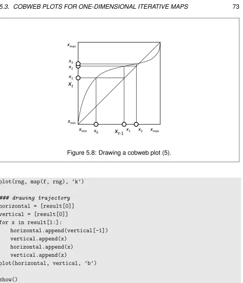
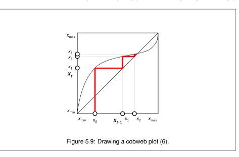
5.3 Cobweb Plots for One-Dimensional Iterative Maps . . . 68
5.4 Graph-Based Phase Space Visualization of Discrete-State Discrete-Time Models . . . 74
5.5 Variable Rescaling . . . 77
5.6 Asymptotic Behavior of Discrete-Time Linear Dynamical Systems . . . 81
5.7 Linear Stability Analysis of Discrete-Time Nonlinear Dynamical Systems . . 90
6 Continuous-Time Models I: Modeling 99 6.1 Continuous-Time Models with Differential Equations . . . 99
6.2 Classifications of Model Equations . . . 100
6.3 Connecting Continuous-Time Models with Discrete-Time Models . . . 102
6.4 Simulating Continuous-Time Models . . . 104
6.5 Building Your Own Model Equation . . . 108
7 Continuous-Time Models II: Analysis 111 7.1 Finding Equilibrium Points . . . 111
7.2 Phase Space Visualization . . . 112
7.3 Variable Rescaling . . . 118
7.4 Asymptotic Behavior of Continuous-Time Linear Dynamical Systems . . . . 120
7.5 Linear Stability Analysis of Nonlinear Dynamical Systems . . . 125
8 Bifurcations 131 8.1 What Are Bifurcations? . . . 131
8.2 Bifurcations in 1-D Continuous-Time Models . . . 132
8.3 Hopf Bifurcations in 2-D Continuous-Time Models . . . 140
8.4 Bifurcations in Discrete-Time Models . . . 144
9 Chaos 153 9.1 Chaos in Discrete-Time Models . . . 153
9.2 Characteristics of Chaos . . . 156
9.3 Lyapunov Exponent . . . 157
CONTENTS xvii
III
Systems with a Large Number of Variables
171
10 Interactive Simulation of Complex Systems 173
10.1 Simulation of Systems with a Large Number of Variables . . . 173
10.2 Interactive Simulation with PyCX . . . 174
10.3 Interactive Parameter Control in PyCX . . . 180
10.4 Simulation without PyCX . . . 181
11 Cellular Automata I: Modeling 185 11.1 Definition of Cellular Automata . . . 185
11.2 Examples of Simple Binary Cellular Automata Rules . . . 190
11.3 Simulating Cellular Automata . . . 192
11.4 Extensions of Cellular Automata . . . 200
11.5 Examples of Biological Cellular Automata Models . . . 201
12 Cellular Automata II: Analysis 209 12.1 Sizes of Rule Space and Phase Space . . . 209
12.2 Phase Space Visualization . . . 211
12.3 Mean-Field Approximation . . . 215
12.4 Renormalization Group Analysis to Predict Percolation Thresholds . . . 219
13 Continuous Field Models I: Modeling 227 13.1 Continuous Field Models with Partial Differential Equations . . . 227
13.2 Fundamentals of Vector Calculus . . . 229
13.3 Visualizing Two-Dimensional Scalar and Vector Fields . . . 236
13.4 Modeling Spatial Movement . . . 241
13.5 Simulation of Continuous Field Models . . . 249
13.6 Reaction-Diffusion Systems . . . 259
14 Continuous Field Models II: Analysis 269 14.1 Finding Equilibrium States . . . 269
14.2 Variable Rescaling . . . 273
14.3 Linear Stability Analysis of Continuous Field Models . . . 275
14.4 Linear Stability Analysis of Reaction-Diffusion Systems . . . 285
15 Basics of Networks 295 15.1 Network Models . . . 295
xviii CONTENTS
15.3 Constructing Network Models with NetworkX . . . 303
15.4 Visualizing Networks with NetworkX . . . 310
15.5 Importing/Exporting Network Data . . . 314
15.6 Generating Random Graphs . . . 320
16 Dynamical Networks I: Modeling 325 16.1 Dynamical Network Models . . . 325
16.2 Simulating DynamicsonNetworks . . . 326
16.3 Simulating DynamicsofNetworks . . . 348
16.4 Simulating Adaptive Networks . . . 360
17 Dynamical Networks II: Analysis of Network Topologies 371 17.1 Network Size, Density, and Percolation . . . 371
17.2 Shortest Path Length . . . 377
17.3 Centralities and Coreness . . . 380
17.4 Clustering . . . 386
17.5 Degree Distribution . . . 389
17.6 Assortativity . . . 396
17.7 Community Structure and Modularity . . . 400
18 Dynamical Networks III: Analysis of Network Dynamics 405 18.1 Dynamics of Continuous-State Networks . . . 405
18.2 Diffusion on Networks . . . 407
18.3 Synchronizability . . . 409
18.4 Mean-Field Approximation of Discrete-State Networks . . . 416
18.5 Mean-Field Approximation on Random Networks . . . 417
18.6 Mean-Field Approximation on Scale-Free Networks . . . 420
19 Agent-Based Models 427 19.1 What Are Agent-Based Models? . . . 427
19.2 Building an Agent-Based Model . . . 431
19.3 Agent-Environment Interaction . . . 440
19.4 Ecological and Evolutionary Models . . . 448
Bibliography 465
Part I
Preliminaries
Chapter 1
Introduction
1.1
Complex Systems in a Nutshell
It may be rather unusual to begin a textbook with an outright definition of a topic, but anyway, here is what we mean bycomplex systemsin this textbook1:
Complex systems are networks made of a number of components that interact with each other, typically in a nonlinear fashion. Complex systems may arise and evolve through self-organization, such that they are neither completely regular nor com-pletely random, permitting the development of emergent behavior at macroscopic scales.
These properties can be found in many real-world systems, e.g., gene regulatory net-works within a cell, physiological systems of an organism, brains and other neural sys-tems, food webs, the global climate, stock markets, the Internet, social media, national and international economies, and even human cultures and civilizations.
To better understand what complex systems are, it might help to know what they are not. One example of systems that are not complex is a collection of independent compo-nents, such as an ideal gas (as discussed in thermodynamics) and random coin tosses (as discussed in probability theory). This class of systems was called “problems of dis-organized complexity”by American mathematician and systems scientist Warren Weaver [2]. Conventional statistics works perfectly when handling such independent entities. An-other example, which is at the An-other extreme, is a collection of strongly coupled compo-1In fact, the first sentence of this definition is just a bit wordier version of Herbert Simon’s famous
def-inition in his 1962 paper [1]: “[A] complex system [is a system] made up of a large number of parts that interact in a nonsimple way.”
4 CHAPTER 1. INTRODUCTION nents, such as rigid bodies (as discussed in classical mechanics) and fixed coin tosses (I’m not sure which discipline studies this). Weaver called this class of systems “prob-lems of simplicity” [2]. In this class, the components of a system are tightly coupled to each other with only a few or no degrees of freedom left within the system, so one can describe the collection as a single entity with a small number of variables. There are very well-developed theories and tools available to handle either case. Unfortunately, however, most real-world systems are somewhere in between.
Complex systems science is a rapidly growing scientific research area that fills the huge gap between the two traditional views that consider systems made of either com-pletely independent or comcom-pletely coupled components. This is the gap where what Weaver called “problems of organized complexity” exist [2]. Complex systems science develops conceptual, mathematical, and computational tools to describe systems made ofinterdependentcomponents. It studies the structural and dynamical properties of vari-ous systems to obtain general, cross-disciplinary implications and applications.
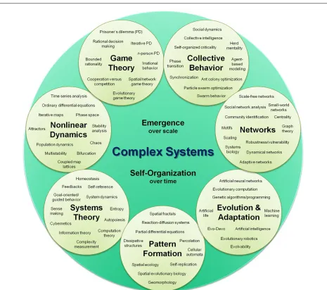
Complex systems science has multiple historical roots and topical clusters of concepts, as illustrated in Fig. 1.1. There are two core concepts that go across almost all subareas of complex systems: emergence and self-organization.
The idea of emergence was originally discussed in philosophy more than a century ago. There are many natural phenomena where some property of a system observed at macroscopic scales simply can’t be reduced to microscopic physical rules that drive the system’s behavior. For example, you can easily tell that a dog wagging its tail is alive, but it is extremely difficult to explain what kind of microscopic physical/chemical processes going on in its body are making this organism “alive.” Another typical example is your consciousness. You know you are conscious, but it is hard to describe what kind of neurophysiological processes make you a “conscious” entity. Those macroscopic properties (livingness, consciousness) are called emergent properties of the systems.
1.1. COMPLEX SYSTEMS IN A NUTSHELL 5
6 CHAPTER 1. INTRODUCTION
Emergence is a nontrivial relationship between the properties of a system at micro-scopic and macromicro-scopic scales. Macromicro-scopic properties are calledemergentwhen it is hard to explain them simply from microscopic properties.
Another key idea of complex systems science is self-organization, which is some-times confused with emergence. Some researchers even use these terms almost in-terchangeably. One clear distinction, though, is that, while emergence is about scale, self-organization is about time (in addition to scale). Namely, you call something self-organizingwhen you observe that the system spontaneously organizes itself to produce a nontrivial macroscopic structure and/or behavior (or “order,” if you will) as time pro-gresses. In other words, self-organization is a dynamical process that looks as if it were going against the second law of thermodynamics (which states that entropy of a closed system increases monotonically over time). Many physical, biological, and social sys-tems show self-organizing behavior, which could appear mysterious when people were not aware of the possibility of self-organization. Of course, these systems are not truly going against the law of thermodynamics, because they are open systems that are driven by energy flow coming from and going to the outside of the system. In a sense, the idea of self-organization gives a dynamical explanation for emergent properties of complex systems.
Self-organization is a dynamical process by which a system spontaneously forms nontrivial macroscopic structures and/or behaviors over time.
Around these two key ideas, there are several topical clusters, which are illustrated in Fig. 1.1. Let’s quickly review them.
1.2
Topical Clusters
1.2. TOPICAL CLUSTERS 7 The possibility of chaotic behavior in such nonlinear systems implies that there will be no analytical solutions generally available for them. This constitutes one of the several origins of the idea of complexity.
Systems theory is another important root of complex systems science. It rapidly de-veloped during and after World War II, when there was a huge demand for mathematical theories to formulate systems that could perform computation, control, and/or communi-cation. This category includes several ground-breaking accomplishments in the last cen-tury, such as Alan Turing’s foundational work on theoretical computer science [7], Norbert Wiener’s cybernetics [8], and Claude Shannon’s information and communication theories [9]. A common feature shared by those theories is that they all originated from some engi-neering discipline, where engineers were facing real-world complex problems and had to come up with tools to meet societal demands. Many innovative ideas of systems thinking were invented in this field, which still form the key components of today’s complex systems science.
Game theoryalso has an interesting societal background. It is a mathematical theory, established by John von Neumann and Oskar Morgenstern [10], which formulates the decisions and behaviors of people playing games with each other. It was developed during the Cold War, when there was a need to seek a balance between the two mega powers that dominated the world at that time. The rationality of the game players was typically assumed in many game theory models, which made it possible to formulate the decision making process as a kind of deterministic dynamical system (in which either decisions themselves or their probabilities could be modeled deterministically). In this sense, game theory is linked to nonlinear dynamics. One of the many contributions game theory has made to science in general is that it demonstrated ways to model and analyze human behavior with great rigor, which has made huge influences on economics, political science, psychology, and other areas of social sciences, as well as contributing to ecology and evolutionary biology.
8 CHAPTER 1. INTRODUCTION Pattern formation is a self-organizing process that involves space as well as time. A system is made of a large number of components that are distributed over a spatial do-main, and their interactions (typically local ones) create an interesting spatial pattern over time. Cellular automata, developed by John von Neumann and Stanisław Ulam in the 1940s [11], are a well-known example of mathematical models that address pattern for-mation. Another modeling framework ispartial differential equations(PDEs) that describe spatial changes of functions in addition to their temporal changes. We will discuss these modeling frameworks later in this textbook.
Evolution andadaptationhave been discussed in several different contexts. One con-text is obviously evolutionary biology, which can be traced back to Charles Darwin’s evo-lutionary theory. But another, which is often discussed more closely to complex systems, is developed in the“complex adaptive systems”context, which involvesevolutionary com-putation,artificial neural networks, and other frameworks of man-made adaptive systems that are inspired by biological and neurological processes. Called soft computing, ma-chine learning, or computational intelligence, nowadays, these frameworks began their rapid development in the 1980s, at the same time when complex systems science was about to arise, and thus they were strongly coupled—conceptually as well as in the lit-erature. In complex systems science, evolution and adaptation are often considered to be general mechanisms that can not only explain biological processes, but also create non-biological processes that have dynamic learning and creative abilities. This goes well beyond what a typical biological study covers.
1.2. TOPICAL CLUSTERS 9 these topical areas will expand further in the coming decades as the understanding of the collective dynamics of complex systems will increase their relevance in our everyday lives.
Here, I should note that these seven topical clusters are based on my own view of the field, and they are by no means well defined or well accepted by the community. There must be many other ways to categorize diverse complex systems related topics. These clusters are more or less categorized based on research communities and subject areas, while the methodologies of modeling and analysis traverse across many of those clusters. Therefore, the following chapters of this textbook are organized based on the methodologies of modeling and analysis, and they are not based on specific subjects to be modeled or analyzed. In this way, I hope you will be able to learn the “how-to” skills systematically in the most generalizable way, so that you can apply them to various subjects of your own interest.
Exercise 1.1 Choose a few concepts of your own interest from Fig. 1.1. Do a quick online literature search for those words, using Google Scholar (http: //scholar.google.com/), arXiv (http://arxiv.org/), etc., to find out more about their meaning, when and how frequently they are used in the literature, and in what context.
Exercise 1.2 Conduct an online search to find visual examples or illustrations of some of the concepts shown in Fig. 1.1. Discuss which example(s) and/or illustra-tion(s) are most effective in conveying the key idea of each concept. Then create a short presentation of complex systems science using the visual materials you selected.
Exercise 1.3 Think of other ways to organize the concepts shown in Fig. 1.1 (and any other relevant concepts you want to include). Then create your own version of a map of complex systems science.
Chapter 2
Fundamentals of Modeling
2.1
Models in Science and Engineering
Science is an endeavor to try to understand the world around us by discovering funda-mental laws that describe how it works. Such laws include Newton’s law of motion, the ideal gas law, Ohm’s law in electrical circuits, the conservation law of energy, and so on, some of which you may have learned already.
A typical cycle of scientific effort by which scientists discover these fundamental laws may look something like this:
1. Observe nature.
2. Develop a hypothesis that could explain your observations.
3. From your hypothesis, make some predictions that are testable through an experi-ment.
4. Carry out the experiment to see if your predictions are actually true.
• Yes→Your hypothesis is proven, congratulations. Uncork a champagne bottle and publish a paper.
• No→Your hypothesis was wrong, unfortunately. Go back to the lab or the field, get more data, and develop another hypothesis.
Many people think this is how science works. But there is at least one thing that is not quite right in the list above. What is it? Can you figure it out?
12 CHAPTER 2. FUNDAMENTALS OF MODELING As some of you may know already, the problem exists in the last part, i.e., when the experiment produced a result that matched your predictions. Let’s do some logic to better understand what the problem really is. Assume that you observed a phenomenon P in nature and came up with a hypothesis H that can explain P. This means that a logical statementH →P is always true (because you chose H that way). To prove H, you also derived a predictionQ fromH, i.e., another logical statementH → Qis always true, too. Then you conduct experiments to see ifQcan be actually observed. What ifQis actually observed? Or, what if “notQ” is observed instead?
If “notQ” is observed, things are easy. Logically speaking, (H → Q)is equivalent to
(notQ → notH) because they are contrapositions of each other, i.e., logically identical statements that can be converted from one to another by negating both the condition and the consequence and then flipping their order. This means that, if not Q is true, then it logically proves that notH is also true, i.e., your hypothesis is wrong. This argument is clear, and there is no problem with it (aside from the fact that you will probably have to redo your hypothesis building and testing).
The real problem occurs when your experiment gives you the desired result, Q. Logi-cally speaking,“(H →Q)andQ” doesn’t tell you anything about whetherH is true or not! There are many ways your hypothesis could be wrong or insufficient even if the predicted outcome was obtained in the experiment. For example, maybe another alternative hy-pothesisRcould be the right one (R→P,R→Q), or maybeHwould need an additional conditionK to predict P and Q(H andK → P, H andK →Q) but you were not aware of the existence ofK.
Let me give you a concrete example. One morning, you looked outside and found that your lawn was wet (observation P). You hypothesized that it must have rained while you were asleep (hypothesis H), which perfectly explains your observation (H → P). Then you predicted that, if it rained overnight, the driveway next door must also be wet (prediction Q that satisfies H → Q). You went out to look and, indeed, it was also wet (if not, H would be clearly wrong). Now, think about whether this new observation really proves your hypothesis that it rained overnight. If you think critically, you should be able to come up with other scenarios in which both your lawn and the driveway next door could be wet without having a rainy night. Maybe the humidity in the air was unusually high, so the condensation in the early morning made the ground wet everywhere. Or maybe a fire hydrant by the street got hit by a car early that morning and it burst open, wetting the nearby area. There could be many other potential explanations for your observation.
2.1. MODELS IN SCIENCE AND ENGINEERING 13 can’t. There is no logical way for us to reach the ground truth of nature1.
This means that all the “laws of nature,” including those listed previously, are no more than well-tested hypotheses at best. Scientists have repeatedly failed to disprove them, so we give them more credibility than we do to other hypotheses. But there is absolutely no guarantee of their universal, permanent correctness. There is always room for other alternative theories to better explain nature.
In this sense, all science can do is just buildmodelsof nature. All of the laws of nature mentioned earlier are also models, not scientific facts, strictly speaking. This is something every single person working on scientific research should always keep in mind.
I have used the word “model” many times already in this book without giving it a defi-nition. So here is an informal definition:
A model is a simplified representation of a system. It can be conceptual, verbal, diagrammatic, physical, or formal (mathematical).
As a cognitive entity interacting with the external world, you are always creating a model of something in your mind. For example, at this very moment as you are reading this textbook, you are probably creating a model of what is written in this book. Modeling is a fundamental part of our daily cognition and decision making; it is not limited only to science.
With this understanding of models in mind, we can say that science is an endless effort to create models of nature, because, after all, modeling is the one and only rational ap-proach to the unreachable reality. And similarly, engineering is an endless effort to control or influence nature to make something desirable happen, by creating and controlling its models. Therefore, modeling occupies the most essential part in any endeavor in science and engineering.
Exercise 2.1 In the “wet lawn” scenario discussed above, come up with a few more alternative hypotheses that could explain both the wet lawn and the wet driveway without assuming that it rained. Then think of ways to find out which hypothesis is most likely to be the real cause.
1This fact is deeply related to the impossibility of general system identification, including the identification
14 CHAPTER 2. FUNDAMENTALS OF MODELING
Exercise 2.2 Name a couple of scientific models that are extensively used in today’s scientific/engineering fields. Then investigate the following:
• How were they developed?
• What made them more useful than earlier models?
• How could they possibly be wrong?
2.2
How to Create a Model
There are a number of approaches for scientific model building. My favorite way of clas-sifying various kinds of modeling approaches is to put them into the following two major families:
Descriptive modeling In this approach, researchers try to specify the actual state of a system at a given time point (or at multiple time points) in a descriptive manner. Taking a picture, creating a miniature (this is literally a “model” in the usual sense of the word), and writing a biography of someone, all belong to this family of modeling effort. This can also be done using quantitative meth-ods (e.g., equations, statistics, computational algorithms), such as regression analysis and pattern recognition. They all try to capture “what the system looks like.”
Rule-based modeling In this approach, researchers try to come up with dynami-cal rules that can explain the observed behavior of a system. This allows re-searchers to make predictions of its possible (e.g., future) states. Dynamical equations, theories, and first principles, which describe how the system will change and evolve over time, all belong to this family of modeling effort. This is usually done using quantitative methods, but it can also be achieved at con-ceptual levels as well (e.g., Charles Darwin’s evolutionary theory). They all try to capture “how the system will behave.”
2.2. HOW TO CREATE A MODEL 15 In the meantime, Newton derived the law of motion to make sense out of observational information, which was a rule-based modeling approach that allowed people to make predictions about how the planets would/could move in the future or in a hypothetical scenario. In other words, descriptive modeling is a process in which descriptions of a system are produced and accumulated, while rule-based modeling is a process in which underlying dynamical explanations are built for those descriptions. These two approaches take turns and form a single cycle of the scientific modeling effort.
In this textbook, we will focus on the latter, the rule-based modeling approach. This is because rule-based modeling plays a particularly important role in complex systems sci-ence. More specifically, developing a rule-based model at microscopic scales and study-ing its macroscopic behaviors through computer simulation and/or mathematical analysis is almost a necessity to understand emergence and self-organization of complex sys-tems. We will discuss how to develop rule-based models and what the challenges are throughout this textbook.
A typical cycle of rule-based modeling effort goes through the following steps (which are similar to the cycle of scientific discoveries we discussed above):
1. Observe the system of your interest.
2. Reflect on the possible rules that might cause the system’s characteristics that were seen in the observation.
3. Derive predictions from those rules and compare them with reality.
4. Repeat the above steps to modify the rules until you are satisfied with the model (or you run out of time or funding).
This seems okay, and it doesn’t contain the logical problem of “proving a hypothesis” that we had before, because I loosened the termination criteria to be your satisfaction as a researcher. However, there is still one particular step that is fundamentally difficult. Which step do you think it is?
16 CHAPTER 2. FUNDAMENTALS OF MODELING Let me give you some examples to illustrate my point. The following figure shows an observation of a system over time. Can you create a mathematical model of this observation?
Time Some quantity
Figure 2.1: Observation example 1.
This one should be quite easy, because the observed data show that nothing changed over time. The description “no change” is already a valid model written in English, but if you prefer writing it in mathematical form, you may want to write it as
x(t) =C (2.1)
or, if you use a differential equation,
dx
dt = 0. (2.2)
Coming up with these models is a no brainer, because we have seen this kind of behavior many times in our daily lives.
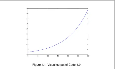
Here is another example. Can you create a mathematical model of this observation?
Time Some quantity
2.2. HOW TO CREATE A MODEL 17 Now we see some changes. It seems the quantity monotonically increased over time. Then your brain must be searching your past memories for a pattern that looks like this curve you are looking at, and you may already have come up with a phrase like “expo-nential growth,”or more mathematically, equations like
x(t) =aebt (2.3)
or
dx
dt =bx. (2.4)
This may be easy or hard, depending on how much knowledge you have about such exponential growth models.
In the meantime, if you show the same curve to middle school students, they may proudly say that this must be the right half of a flattened parabola that they just learned about last week. And there is nothing fundamentally wrong with that idea. It could be a right half of a parabola, indeed. We never know for sure until we see what the entire curve looks like for−∞< t <∞.
Let’s move on to a more difficult example. Create a mathematical model of the follow-ing observation.
Time Some quantity
Figure 2.3: Observation example 3.
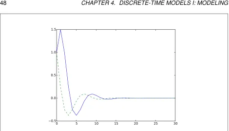
18 CHAPTER 2. FUNDAMENTALS OF MODELING This last example is the toughest. Create a mathematical model of the following ob-servation.
Time Some quantity
Figure 2.4: Observation example 4.
Did you come up with any ideas? I have seen only a few people who were able to make reasonable models of this observation throughout my career. The reason why this example is so hard to model is because we don’t see this kind of behavior often in our lives. We are simply not experienced with it. We don’t have a good mental template to use to capture the essence of this pattern2.
I hope that these examples have made my point clear by now. Coming up with a model is inherently a personal process, which depends on your own knowledge, experience, and worldview. There is no single algorithm or procedure you can follow to develop a good model. The modeling process is a full-scale interaction between the external world and your whole, intellectual self. To become a good modeler, you will need to gain diverse knowledge and experience and develop rich worldviews. This is why I said it would be very difficult to be taught.
Exercise 2.3 Create a few different models for each of the examples shown above. Discuss how those models differ from each other, and what you should do to determine which model is more appropriate as an explanation of the observed behavior.
2For those who are curious—this kind of curve could be generated by raising a sine or cosine function of
time to an odd number (e.g.,sin3(t),cos5(t)), but I am not sure if knowing this would ever help you in your
2.3. MODELING COMPLEX SYSTEMS 19
2.3
Modeling Complex Systems
The challenge in developing a model becomes particularly tough when it comes to the modeling of complex systems, because their unique properties (networks, nonlinearity, emergence, self-organization, etc.) are not what we are familiar with. We usually think about things on a single scale in a step-by-step, linear chain of reasoning, in which causes and effects are clearly distinguished and discussed sequentially. But this approach is not suitable for understanding complex systems where a massive amount of components are interacting with each other interdependently to generate patterns over a broad range of scales. Therefore, the behavior of complex systems often appears to contradict our everyday experiences.
As illustrated in the examples above, it is extremely difficult for us to come up with a reasonable model when we are facing something unfamiliar. And it is even more difficult to come up with a reasonable set of microscopic rules that could explain the observed macroscopic properties of a system. Most of us are simply not experienced enough to make logical connections between things at multiple different scales.
How can we improve our abilities to model complex systems? The answer might be as simple as this: We need to become experienced and familiar with various dynamics of complex systems to become a good modeler of them. How can we become experi-enced? This is a tricky question, but thanks to the availability of the computers around us, computational modeling and simulation is becoming a reasonable, practical method for this purpose. You can construct your own model with full details of microscopic rules coded into your computer, and then let it actually show the macroscopic behavior aris-ing from those rules. Such computational modelaris-ing and simulation is a very powerful tool that allows you to gain interactive, intuitive (simulated) experiences of various possi-ble dynamics that help you make mental connections between micro- and macroscopic scales. I would say there are virtually no better tools available for studying the dynamics of complex systems in general.
There are a number of pre-built tools available for complex systems modeling and simulation, including NetLogo [13], Repast [14], MASON [15], Golly [16], and so on. You could also build your own model by using general-purpose computer programming lan-guages, including C, C++, Java, Python, R, Mathematica, MATLAB, etc. In this textbook, we choose Python as our modeling tool, specifically Python 2.7, and use PyCX [17] to build interactive dynamic simulation models3. Python is free and widely used in scien-3For those who are new to Python programming, see Python’s online tutorial athttps://docs.python.
20 CHAPTER 2. FUNDAMENTALS OF MODELING tific computing as well as in the information technology industries. More details of the rationale for this choice can be found in [17].
When you create a model of a complex system, you typically need to think about the following:
1. What are the key questions you want to address?
2. To answer those key questions, at what scale should you describe the behaviors of the system’s components? These components will be the “microscopic” compo-nents of the system, and you will define dynamical rules for their behaviors.
3. How is the system structured? This includes what those microscopic components are, and how they will be interacting with each other.
4. What are the possible states of the system? This means describing what kind of dynamical states each component can take.
5. How does the state of the system change over time? This includes defining the dynamical rules by which the components’ states will change over time via their mutual interaction, as well as defining how the interactions among the components will change over time.
Figuring out the “right” choices for these questions is by no means a trivial task. You will likely need to loop through these questions several times until your model successfully produces behaviors that mimic key aspects of the system you are trying to model. We will practice many examples of these steps throughout this textbook.
Exercise 2.4 Create a schematic model of some real-world system of your choice that is made of many interacting components. Which scale do you choose to de-scribe the microscopic components? What are those components? What states can they take? How are those components connected? How do their states change over time? After answering all of these questions, make a mental prediction about what kind of macroscopic behaviors would arise if you ran a computational simulation of your model.
2.4. WHAT ARE GOOD MODELS? 21
2.4
What Are Good Models?
You can create various kinds of models for a system, but useful ones have several impor-tant properties. Here is a very brief summary of what a good model should look like:
A good model is simple, valid, and robust.
Simplicity of a model is really the key essence of what modeling is all about. The main reason why we want to build a model is that we want to have a shorter, simpler description of reality. As the famous principle of Occam’s razor says, if you have two models with equal predictive power, you should choose the simpler one. This is not a theorem or any logically proven fact, but it is a commonly accepted practice in science. Parsimony is good because it is economical (e.g., we can store more models within the limited capacity of our brain if they are simpler) and also insightful (e.g., we may find useful patterns or applications in the models if they are simple). If you can eliminate any parameters, variables, or assumptions from your model without losing its characteristic behavior, you should.
Validity of a model is how closely the model’s prediction agrees with the observed reality. This is of utmost importance from a practical viewpoint. If your model’s prediction doesn’t reasonably match the observation, the model is not representing reality and is probably useless. It is also very important to check the validity of not only the predictions of the model but also the assumptions it uses, i.e., whether each of the assumptions used in your model makes sense at its face value, in view of the existing knowledge as well as our common sense. Sometimes this “face validity” is more important in complex systems modeling, because there are many situations where we simply can’t conduct a quantitative comparison between the model prediction and the observational data. Even if this is the case, you should at least check the face validity of your model assumptions based on your understanding about the system and/or the phenomena.
Note that there is often a trade-off between trying to achieve simplicity and validity of a model. If you increase the model complexity, you may be able to achieve a better fit to the observed data, but the model’s simplicity is lost and you also have the risk ofoverfitting— that is, the model prediction may become adjusted too closely to a specific observation at the cost of generalizability to other cases. You need to strike the right balance between those two criteria.
22 CHAPTER 2. FUNDAMENTALS OF MODELING the real world. If the prediction made by your model is sensitive to their minor variations, then the conclusion derived from it is probably not reliable. But if your model is robust, the conclusion will hold under minor variations of model assumptions and parameters, therefore it will more likely apply to reality, and we can put more trust in it.
Exercise 2.5 Humanity has created a number of models of the solar system in its history. Some of them are summarized below:
• Ptolemy’s geocentric model (which assumes that the Sun and other planets are revolving around the Earth)
• Copernicus’ heliocentric model (which assumes that the Earth and other plan-ets are revolving around the Sun in concentric circular orbits)
• Kepler’s laws of planetary motion (which assumes that the Earth and other planets are revolving in elliptic orbits, at one of whose foci is the Sun, and that the area swept by a line connecting a planet and the Sun during a unit time period is always the same)
• Newton’s law of gravity (which assumes that a gravitational force between two objects is proportional to their masses and inversely proportional to their distance squared)
Investigate these models, and compare them in terms of simplicity, validity and robustness.
2.5
A Historical Perspective
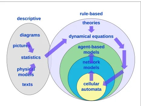
As the final section in this chapter, I would like to present some historical perspective of how people have been developing modeling methodologies over time, especially those for complex systems (Fig. 2.5). Humans have been creating descriptive models (diagrams, pictures, physical models, texts, etc.) and some conceptual rule-based models since ancient times. More quantitative modeling approaches arose as more advanced mathe-matical tools became available. In the descriptive modeling family, descriptive statistics is among such quantitative modeling approaches. In the rule-based modeling family, dy-namical equations (e.g., differential equations, difference equations) began to be used to quantitatively formulate theories that had remained at conceptual levels before.
2.5. A HISTORICAL PERSPECTIVE 23
descriptive
rule-based
statistics
diagrams
pictures
physical
models
texts
theories
dynamical equations
agent-based
models
network
models
cellular
automata
24 CHAPTER 2. FUNDAMENTALS OF MODELING for complex systems modeling. The first of this kind was cellular automata, a massive number of identical finite-state machines that are arranged in a regular grid structure and update their states dynamically according to their own and their neighbors’ states. Cel-lular automata were developed by John von Neumann and Stanisław Ulam in the 1940s, initially as a theoretical medium to implement self-reproducing machines [11], but later they became a very popular modeling framework for simulating various interesting emer-gent behaviors and also for more serious scientific modeling of spatio-temporal dynamics [18]. Cellular automata are a special case of dynamical networks whose topologies are limited to regular grids and whose nodes are usually assumed to be homogeneous and identical.
Dynamical networks formed the next wave of complex systems modeling in the 1970s and 1980s. Their inspiration came from artificial neural networkresearch by Warren Mc-Culloch and Walter Pitts [19] as well as by John Hopfield [20, 21], and also from theoretical gene regulatory networkresearch by Stuart Kauffman [22]. In this modeling framework, the topologies of systems are no longer constrained to regular grids, and the components and their connections can be heterogeneous with different rules and weights. Therefore, dynamical networks include cellular automata as a special case within them. Dynamical networks have recently merged with another thread of research on topological analysis that originated in graph theory, statistical physics, social sciences, and computational sci-ence, to form a new interdisciplinary field ofnetwork science[23, 24, 25].
Finally, further generalization was achieved by removing the requirement of explicit network topologies from the models, which is now called agent-based modeling(ABM). In ABM, the only requirement is that the system is made of multiple discrete “agents” that interact with each other (and possibly with the environment), whether they are structured into a network or not. Therefore ABM includes network models and cellular automata as its special cases. The use of ABM became gradually popular during the 1980s, 1990s, and 2000s. One of the primary driving forces for it was the application of complex sys-tems modeling to ecological, social, economic, and political processes, in fields like game theory and microeconomics. The surge ofgenetic algorithmsand other population-based search/optimization algorithms in computer science also took place at about the same time, which also had synergistic effects on the rise of ABM.
2.5. A HISTORICAL PERSPECTIVE 25
Part II
Systems with a Small Number of
Variables
Chapter 3
Basics of Dynamical Systems
3.1
What Are Dynamical Systems?
Dynamical systems theoryis the very foundation of almost any kind of rule-based models of complex systems. It considers how systems change over time, not just static properties of observations. A dynamical system can be informally defined as follows1:
A dynamical system is a system whose state is uniquely specified by a set of variables and whose behavior is described by predefined rules.
Examples of dynamical systems include population growth, a swinging pendulum, the motions of celestial bodies, and the behavior of “rational” individuals playing a negotiation game, to name a few. The first three examples sound legitimate, as those are systems that typically appear in physics textbooks. But what about the last example? Could hu-man behavior be modeled as a deterministic dynamical system? The answer depends on how you formulate the model using relevant assumptions. If you assume that individuals make decisions always perfectly rationally, then the decision making process becomes deterministic, and therefore the interactions among them may be modeled as a determin-istic dynamical system. Of course, this doesn’t guarantee whether it is a good model or not; the assumption has to be critically evaluated based on the criteria discussed in the previous chapter.
Anyway, dynamical systems can be described over either discrete time steps or a continuous time line. Their general mathematical formulations are as follows:
1A traditional definition of dynamical systems considers deterministic systems only, but stochastic (i.e.,
probabilistic) behaviors can also be modeled in a dynamical system by, for example, representing the prob-ability distribution of the system’s states as a meta-level state.
30 CHAPTER 3. BASICS OF DYNAMICAL SYSTEMS
Discrete-time dynamical system
xt=F(xt−1, t) (3.1)
This type of model is called adifference equation, arecurrence equation, or an iterative map(if there is noton the right hand side).
Continuous-time dynamical system
dx
dt =F(x, t) (3.2)
This type of model is called adifferential equation.
In either case,xtorxis thestate variableof the system at timet, which may take a scalar
or vector value. F is a function that determines the rules by which the system changes its state over time. The formulas given above are first-order versions of dynamical sys-tems (i.e., the equations don’t involve xt−2, xt−3, . . ., or d2x/dt2, d3x/dt3, . . .). But these
first-order forms are general enough to cover all sorts of dynamics that are possible in dynamical systems, as we will discuss later.
Exercise 3.1 Have you learned of any models in the natural or social sciences that are formulated as either discrete-time or continuous-time dynamical systems as shown above? If so, what are they? What are the assumptions behind those models?
Exercise 3.2 What are some appropriate choices for state variables in the follow-ing systems?
• population growth
• swinging pendulum
• motions of celestial bodies
3.2. PHASE SPACE 31
3.2
Phase Space
Behaviors of a dynamical system can be studied by using the concept of aphase space, which is informally defined as follows:
A phase space of a dynamical system is a theoretical space where every state of the system is mapped to a unique spatial location.
The number of state variables needed to uniquely specify the system’s state is called the degrees of freedom in the system. You can build a phase space of a system by having an axis for each degree of freedom, i.e., by taking each state variable as one of the orthogonal axes. Therefore, the degrees of freedom of a system equal the dimensions of its phase space. For example, describing the behavior of a ball thrown upward in a frictionless vertical tube can be specified with two scalar variables, the ball’s position and velocity, at least until it hits the bottom again. You can thus create its phase space in two dimensions, as shown in Fig. 3.1.
Position x
Velocity v
Position x
V
eloc
it
y
v
Figure 3.1: A ball thrown upward in a vertical tube (left) and a schematic illustration of its phase space (right). The dynamic behavior of the ball can be visualized as a static trajectory in the phase space (red arrows).
32 CHAPTER 3. BASICS OF DYNAMICAL SYSTEMS
Exercise 3.3 In the example above, when the ball hits the floor in the vertical tube, its kinetic energy is quickly converted into elastic energy (i.e., deformation of the ball), and then it is converted back into kinetic energy again (i.e., upward velocity). Think about how you can illustrate this process in the phase space. Are the two dimensions enough or do you need to introduce an additional dimension? Then try to illustrate the trajectory of the system going through a bouncing event in the phase space.
3.3
What Can We Learn?
There are several important things you can learn from phase space visualizations. First, you can tell from the phase space what will eventually happen to a system’s state in the long run. For a deterministic dynamical system, its future state is uniquely determined by its current state (hence, the name “deterministic”). Trajectories of a deterministic dynam-ical system will never branch off in its phase space (though they could merge), because if they did, that would mean that multiple future states were possible, which would vio-late the deterministic nature of the system. No branching means that, once you specify an initial state of the system, the trajectory that follows is uniquely determined too. You can visually inspect where the trajectories are going in the phase space visualization. They may diverge to infinity, converge to a certain point, or remain dynamically chang-ing yet stay in a confined region in the phase space from which no outgochang-ing trajectories are running out. Such a converging point or a region is called an attractor. The concept of attractors is particularly important for understanding the self-organization of complex systems. Even if it may look magical and mysterious, self-organization of complex sys-tems can be understood as a process whereby the system is simply falling into one of the attractors in a high-dimensional phase space.
3.3. WHAT CAN WE LEARN? 33 Another thing you can learn from phase space visualizations is the stability of the system’s states. If you see that trajectories are converging to a certain point or area in the phase space, that means the system’s state is stable in that area. But if you see trajectories are diverging from a certain point or area, that means the system’s state is unstable in that area. Knowing system stability is often extremely important to understand, design, and/or control systems in real-world applications. The following chapters will put a particular emphasis on this stability issue.
Exercise 3.4 Where are the attractor(s) in the phase space of the bouncing ball example created in Exercise 3.3? Assume that every time the ball bounces it loses a bit of its kinetic energy.
Exercise 3.5 For each attractor obtained in Exercise 3.4 above, identify its basin of attraction.
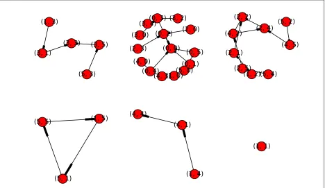
Exercise 3.6 For each of the phase spaces shown below, identify the following:
• attractor(s)
• basin of attraction for each attractor
• stability of the system’s state at several locations in the phase space
34 CHAPTER 3. BASICS OF DYNAMICAL SYSTEMS
where users of each product submit their ratings. Since there is no actual differ-ence in the product quality, the average rating scores are about the same between the two products, but the customers can also see the total number of submitted ratings for each product, which shows how popular the product is in the market. Customers tend to adopt a more popular choice. Answer the following questions:
• What would the phase space of this system look like?
• Are there any attractors? Are there any basins of attraction?
• How does the system’s fate depend on its initial state?
Chapter 4
Discrete-Time Models I: Modeling
4.1
Discrete-Time Models with Difference Equations
Discrete-time modelsare easy to understand, develop and simulate. They are easily im-plementable for stepwise computer simulations, and they are often suitable for modeling experimental data that are almost always already discrete. Moreover, they can repre-sent abrupt changes in the system’s states, and possibly chaotic dynamics, using fewer variables than their continuous-time counterparts (this will be discussed more in Chapter 9).
The discrete-time models of dynamical systems are often calleddifference equations, because you can rewrite any first-order discrete-time dynamical system with a state vari-ablex(Eq. (3.1)), i.e.,
xt=F(xt−1, t) (4.1)
into a “difference” form
∆x=xt−xt−1 =F(xt−1, t)−xt−1, (4.2)
which is mathematically more similar to differential equations. But in this book, we mostly stick to the original form that directly specifies the next value ofx, which is more straight-forward and easier to understand.
Note that Eq. (4.1) can also be written as
xt+1 =F(xt, t), (4.3)
which is mathematically equivalent to Eq. (4.1) and perhaps more commonly used in the literature. But we will use the notation with xt, xt−1, xt−2, etc., in this textbook, because