THREE-DIMENSIONAL VIRTUAL CONCRETE
by
Stephen Thomas
A thesis
submitted in partial fulfillment of the requirements for the degree of
Master of Science in Materials Science and Engineering Boise State University
BOISE STATE UNIVERSITY GRADUATE COLLEGE
DEFENSE COMMITTEE AND FINAL READING APPROVALS
of the thesis submitted by
Stephen Thomas
Thesis Title: Improving and Augmenting the Anm Model for Three-Dimensional Virtual Concrete
Date of Final Oral Examination: 07 March 2017
The following individuals read and discussed the thesis submitted by student Stephen Thomas, and they evaluated his presentation and response to questions during the final oral examination. They found that the student passed the final oral examination.
Yang Lu, Ph.D. Co-Chair, Supervisory Committee
Janet Callahan, Ph.D. Co- Chair, Supervisory Committee Peter Mullner, Ph.D. Member, Supervisory Committee
iv DEDICATION
v
ACKNOWLEDGEMENTS
I would like to thank Dr. Yang Lu for giving me the opportunity to work with him and the guidance he provided during this research. I would like to thank Dr. E.J. Garboczi for his collaboration and contributions on this research. I would like to extend my
gratitude to my exceptional colleagues who have positively influenced my academic and research experience in Boise State University: Mathew Swenson, Tony Valayil Varghese, Chad Watson, Dr. Will Hughes and many more. I would like to thank the Micron School of Materials Science and Engineering staff and the Department of Civil Engineering staff for the support they provided. Last, but not the least, I thank Dr. Janet Callahan and Dr. Peter Mullner for agreeing to be on my committee and guiding me.
vi ABSTRACT
The Anm model used for creating virtual concrete consisting of irregular shapes has been improved by integrating two existing algorithms: the extent overlap box (EOB) method for detecting contact between two irregular shapes and the uniform thickness shell algorithm. The EOB method has been compared with the previously used Newton-Raphson method and shown to be able to detect inter-particle contact with better
vii
can be larger than the prescribed normal distance from the particle surface and this is dependent on the angle between the slice and the particle surface normal. The 2D
viii
TABLE OF CONTENTS
DEDICATION ... iv
ACKNOWLEDGEMENTS ...v
ABSTRACT ... vi
LIST OF TABLES ...x
LIST OF FIGURES ... xi
LIST OF ABBREVIATIONS ... xiv
CHAPTER ONE: INTRODUCTION ...1
1.1 Background ...1
1.2 State of the art ...2
1.3 Research Objectives ...13
1.4 References ...14
CHAPTER TWO: IMPROVED MODEL FOR THREE-DIMENSIONAL VIRTUAL CONCRETE: ANM MODEL ...17
Abstract ...19
2.1 Introduction ...20
2.2 Integration of New Search Algorithm...27
2.3 Integration of the Uniform-Thickness Shell Algorithm into Anm ...34
2.4 Parallel Optimization of Anm Code for Faster Execution ...38
2.5 Results and Discussion ...40
ix
2.5.2 Uniform-Thickness Shell ...43
2.5.3 Effect of Random Locations on Packing Density and Particle Size Distribution ...48
2.5.4 Performance Comparison ...51
2.6 Conclusions and Future Research ...54
2.7 Author Justifications ...55
2.8 References ...56
CHAPTER THREE: IMPLICATIONS OF OVERLAPPING UNIFORM-THICKNESS SHELLS IN THE ANM MODEL ...60
3.1 Introduction ...60
3.2 Overlapping Uniform Thickness Shell ...61
3.3 2D Slicing and Visualization of The Anm Model ...64
3.4 Characterizing the wall effect ...69
3.5 Summary ...84
3.6 References ...85
CHAPTER FOUR: CONCLUSIONS...86
4.1 Innovative Contributions of this Research ...86
4.2 Summary and Outlook ...87
x
LIST OF TABLES
Table 2.1 Particle size distribution and achieved volume fraction by particles from individual sieves... 45 Table 2.2. Number of particles per sieve with respect to the change in shell thickness
of the individual particles... 46 Table 2.3. Changes in PD and PSD of the Anm model as the number of random
locations attempted for each particle is increased. ... 49 Table 3.1 PSD and achieved volume fraction by Μsand. The first column describes
the minimum and maximum width of the particles in that sieve. ... 75 Table 3.2 PSD and achieved volume fraction by Μsand where particles from Sieve
3 were assumed to be spherical particles by reducing the order of Anm coefficients used to 0 instead of 5. The first column describes the
xi
LIST OF FIGURES
Fig. 1.1 3D volume of a multi aggregate sample obtained by X-ray CT scanning. Reproduced from (Garboczi, 2002) ... 4 Fig. 1.2 Aggregate shape in voxel representation (top) and spherical harmonic
expansion reconstruction (below). Reproduced from (Garboczi, 2002)... 6 Fig. 1.3. Flow chart illustrating the packing algorithm used by the Anm model.
Reproduced from (Qian, 2012) ... 7 Fig. 1.4. 2D contact problem involving two circles. Reproduced from (Qian, 2012)
... 8 Fig. 1.5. 2D schematic showing particles overlapping(left) and not
overlapping(right) within the EOB. Reprinted from (Garboczi and Bullard, 2013) ... 10 Fig. 1.6. 2D schematic showing the contact detection algorithm within EOB. ... 11 Fig. 2.1. Placing star-shaped particles to model material mesostructure of mortar or
concrete. ... 24 Fig. 2.2. Three-step algorithm for searching contact. ... 28 Fig. 2.3. Two particles with minimal overlap. ... 29 Fig. 2.4. Schematic representation of particles with overlap along line of centers
shown in 2 dimensions. Here the sum of the individual radii ( r1 + r2 ) is greater than the length of the line of centers. ... 29 Fig. 2.5. Schematic representation of two particles which do not overlap along the
line of center points in 2 dimensions, but have a non-zero volume EOB. 30 Fig. 2.6. Extent box for an irregular shaped particle. ... 31 Fig. 2.7. Illustration of Nbox value. ... 32
Fig. 2.8. A two-dimensional illustration of the Doverlap with respect to two
xii
Fig. 2.9. Adding a shell by increasing the length of the radius vector by different amounts at different original surface points. ... 35 Fig. 2.10. Illustration of the vector equation with three unknowns β, θ' and ∅'. ... 36 Fig. 2.11. Irregular particle with shell of thickness t = 0.2 % of particle length. ... 36 Fig. 2.12. Pseudo code for a typical serial code containing time consuming loops. . 39 Fig. 2.13. Pseudo code for time consuming loops after parallelization. ... 39 Fig. 2.14. The effect of the value of Next on Vbox for a single irregular shaped
particle... 41 Fig. 2.15. The value of Doverlap increases as the value of Nbox increases for two
particles with minimal overlap. The value of Next was fixed at 80 for this
measurement. ... 42 Fig. 2.16. Illustration of the (a) decreasing trend in PD and (b) number of particles
packed with the increase in shell thickness... 47 Fig. 2.17. Illustration of the linear increase in shell volume fraction with the increase in shell thickness. ... 47 Fig. 2.18. Comparison of time taken to rotate a particle using serial and parallel
execution (8 processors) of the algorithm. ... 51 Fig. 2.19. Comparison of the EOB contact searching algorithm using serial and
parallel execution (8 processors). ... 52 Fig. 2.20. Efficiency of contact searching algorithm where the number of
participating processors p=8. ... 53 Fig. 3.1. Flowchart for parking procedure with non-overlapping shells. ... 62 Fig. 3.2 Schematic of a particle-slice overlap. Position p1 on the slice is
overlapped by the particle. The dotted line shown part of the particle behind the slice. Position p2 is not overlapped by the particle. r1 and r2 are surface points on the surface of the particle along the direction of points p1 and p2. ... 66 Fig. 3.3. 2D slice image of overlapping shells obtained from the Anm model (a)
xiii
Fig. 3.4. 2D slice image of varying thickness of the shells on high angle slice planes obtained from the Anm model (left) and the corresponding particles and slice (shown as the black curve) in 3D... 68 Fig. 3.5. Illustration of the “wall effect”. A is a penetrable wall and B is an
impenetrable wall. The packing density near wall B is lower than wall A. (Scrivener, Crumbie and Laugesen, 2004) ... 69 Fig. 3.6. 3D visualization of Anm model 1 where only particles from Sieve 1 (blue)
and Sieve 2 (green) are shown. The particle for which the RDF is
calculated is shown with the uniform thickness shell (light blue) around it. ... 77 Fig. 3.7. Illustration of a mask image superimposed on a corresponding 2D slice of
the Anm model 1 passing through the coarse aggregate for which the RDF is measured. The ten uniform thickness shells are colored with pseudo colors and the particles are shown in black. ... 78 Fig. 3.8. The RDF calculated for one coarse aggregate with a slice density of 1. .. 79 Fig. 3.9. The RDF calculated for one coarse aggregate with four different slice
densities. Slice density of 1 corresponds to Rs of 0.05 mm/pixel. ... 80 Fig. 3.10. Variation in standard deviation of the RDF with increasing slice
density(ρs). Four distances from the particle surface is considered. Slice density of 1 corresponds to Rs of 0.05 mm/pixel. ... 81 Fig. 3.11. The RDF calculated for one coarse aggregate and spherical sand particles
with a slice density of 1. ... 83 Fig. 3.12. The RDF calculated for one coarse aggregate with four different slice
densities with spherical sand particles. Slice density of 1 corresponds to
Rs of 0.05 mm/pixel. ... 83 Fig. 3.13. Variation in standard deviation of the RDF with increasing slice
xiv
LIST OF ABBREVIATIONS
EOB Extent Overlap Box
ITZ Interfacial Transition Zone
API Application Programming Interface PSD Particle Size Distribution
PD Packing Density
NR Newton-Raphson
Next The number of equally spaced polar and azimuthal angles to scan
the particle to find the six extrema of the EOB.
Nbox The number of equally spaced polar and azimuthal angles to scan
the EOB to detect contact of particles. PPL Microsoft Parallel Patterns Library
CHAPTER ONE: INTRODUCTION
This chapter consists of three sections. The first section describes the background and the motivation of this research. The second section describes the state of the art of this research area. In the third section, the research objectives are presented.
1.1Background
Concrete is the most widely used man-made material today and humans used it as early as the ancient Greeks (Jackson et al., 2011). However, there is still much to be elucidated at the micro and nano scale of this material. At the nanoscale, the major phase of cement paste, the calcium-silicate-hydrate (C-S-H) phase is considered a
heterogeneous material. The study of C-S-H is an active area of research (Pellenq et al., 2009; Masoero et al., 2014). At the microscale, concrete is a heterogeneous material with either two or three phases. The two-phase model considers mortar as the matrix and coarse aggregates as the inclusions. The three-phase model considers cement paste as the matrix with both fine aggregates (sand) and coarse aggregates as the inclusions.
A true understanding of concrete requires a multiscale approach. Robust
properties that govern the long-term deflections and the properties associated with failure. Even for linear elastic behavior of cementitious materials, theoretically predicting the composite elastic modulus tensor is non-trivial (Haecker et al., 2005).
Irrespective of which type of physical property is of concern and the type of simulation method used, one of the important constituents of the microscale model is the microstructure. The microstructural model considers details such as phase volume fractions, particle gradation and porosity. Software packages such as CEMHYD3D (Bentz, 1997) and the Virtual Cement and Concrete Testing Laboratory (VCCTL) (Bentz
et al., 2006; Bullard and Garboczi, 2006) use an initial microstructure as the input to predict various properties of cement and concrete. These predictions rely heavily on the accuracy of the input model. These software packages consider three dimensional models since unlike phase volume fractions which are same in two and three dimensions,
connectivity and percolation of phases are different in two and three dimensions. Due to these factors, mechanical and transport behavior are predicted more accurately using three dimensional models.
1.2State of the art
varying particle size distribution (PSD) and packing density (PD) which are key factors describing the microstructure and have real-world implications. For instance, a less dense packing of aggregates requires more cement paste to fill in the voids, thereby increasing the cost of the concrete mix.
Beyond the virtual model affecting the flexibility of varying PSD and PD, the virtual model also is computationally more efficient. The CT scanned models are usually voxel based 3D volumes where the entire volume of the specimen, including the matrix and inclusions must be digitally stored. In contrast, virtual microstructure models usually store just the positions, sizes, orientation, and the shape information of the inclusions. The hard-core soft-shell model (Bentz, Garboczi and Snyder, 1999) is an example of such a model. It is apparent that the shape information is trivial to obtain and store for regular shapes such as spheres and ellipsoids. Typically, the virtual models randomly pack the shapes into a given volume while making sure that the shapes do not overlap each other when the shapes represent inclusions such as aggregates. Again, it is obvious that functions for detecting contact are readily available for regular shapes.
aggregate samples followed by fitting the extracted shapes to spherical harmonic functions (Garboczi, 2002).
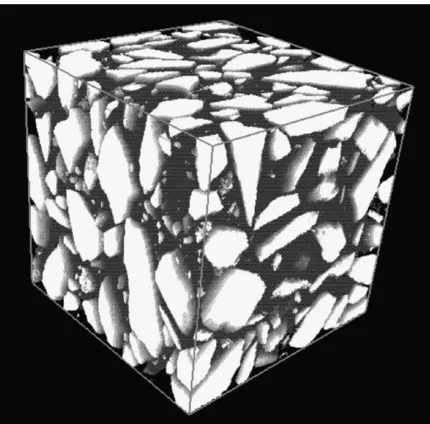
The starting point for this method is a 3D volume such as shown in Fig. 1.1, acquired using X-ray CT scanning. The black voxels represent the matrix and unresolved fine aggregates whereas the white pixels represent the coarse aggregates. The individual particle voxels are then identified using a procedure called the “burning algorithm” (Garboczi, 2002) and extracted for spherical harmonic analysis.
Next, the distance 𝑅(𝜃𝑖, 𝜙𝑖) from the center of mass of individual particles to the surface along a finite number of angles (𝜃𝑖, 𝜙𝑖) in the polar coordinate system are numerically obtained and recorded in a database. Once the surface points 𝑅(𝜃𝑖, 𝜙𝑖) of a particle are identified, spherical harmonic analysis is applied to obtain a function for the shape as shown in Eq. 1.1. Here 𝑟(𝜃, 𝜙) is known from 𝑅(𝜃𝑖, 𝜙𝑖) and 𝑌𝑛𝑚(𝜃, 𝜙) are a set of predefined functions known as the spherical harmonic functions as shown in Eq. 1.2 where 𝑃𝑛𝑚 is a set of orthogonal Legendre polynomials. Spherical harmonic analysis is the 3D equivalent of Fourier analysis in 2D and the spherical harmonic functions are readily available from software packages such as the Boost C++ library (Schaling, 2014).
𝑟(𝜃, 𝜙) = ∑ ∑ 𝑎𝑛𝑚𝑌𝑛𝑚(𝜃, 𝜙) 𝑛 𝑚=−𝑛 . ∞ 𝑛=0 1.1 𝑌𝑛𝑚(𝜃, 𝜙) = √(
(2𝑛 + 1)(𝑛 − 𝑚)! 4𝜋(𝑛 + 𝑚)! ) 𝑃𝑛
𝑚(cos(𝜃))𝑒𝑖𝑚𝜙 1.2
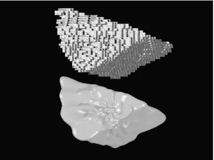
The coefficients 𝑎𝑛𝑚 are obtained for each particle by solving Eq. 1.1 for a finite value of n. Larger values of n gives a better approximation of the original shape. The error in approximation has been shown (Garboczi, 2002) to be negligible above n=12 for the aggregate shape shown in Fig. 1.2 which depicts the aggregate shape in voxel
Fig. 1.2 Aggregate shape in voxel representation (top) and spherical harmonic expansion reconstruction (below). Reproduced from (Garboczi, 2002)
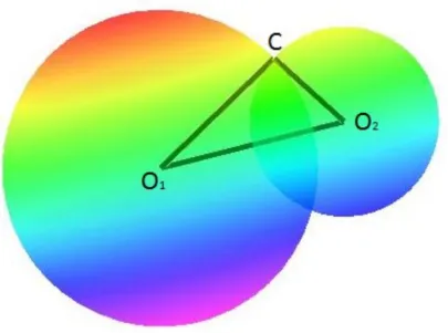
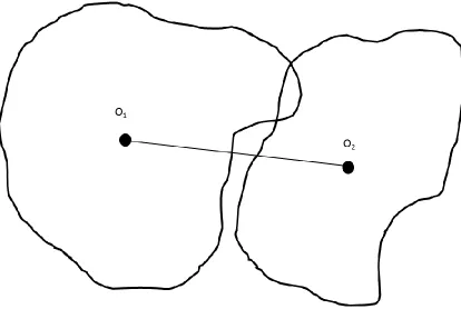
One of the most critical and time consuming steps in this algorithm is the one where the placed particle is checked for overlap with any existing particles in the packed volume. In practice, not all the existing particles are checked for contact. The volume is logically divided into spatial bins and each particle being placed is assigned a bin and the overlap check is only performed on particles that belong to the bin where the new particle is being placed. The method used by the Anm model to detect contact between two particles can be understood through a sphere contact problem illustrated in Fig. 1.4.
Fig. 1.4. 2D contact problem involving two circles. Reproduced from (Qian, 2012)
Here the center of mass of sphere 1 and sphere 2 are 𝑂1(𝑥1, 𝑦1, 𝑧1) and
polar coordinates of each sphere with their center of masses taken as the origins as shown in Eq. 1.3 and 1.4 where 𝑟1 and 𝑟2 are equivalent to the line segments 𝑂1𝐶 and 𝑂2𝐶 in Fig. 1.4.
{
𝑥𝑐 = 𝑥1 + 𝑟1(𝜃1, 𝜙1) sin 𝜃1cos 𝜙1
𝑦𝑐 = 𝑦1+ 𝑟1(𝜃1, 𝜙1) sin 𝜃1sin 𝜙1
𝑧𝑐 = 𝑧1+ 𝑟1(𝜃1, 𝜙1) cos 𝜃1
1.3
{
𝑥𝑐 = 𝑥2+ 𝑟2(𝜃2, 𝜙2) sin 𝜃2cos 𝜙2
𝑦𝑐 = 𝑦2 + 𝑟2(𝜃2, 𝜙2) sin 𝜃2sin 𝜙2
𝑧𝑐 = 𝑧2+ 𝑟2(𝜃2, 𝜙2) cos 𝜃2
1.4
Equating Eq. 1.3 and 1.4, a system of equations Eq. 1.5 is obtained which can be solved to obtain the unknowns 𝜃1, 𝜙1, 𝜃2, 𝜙2.
{
𝑥1+ 𝑟1(𝜃1, 𝜙1) sin 𝜃1cos 𝜙1 = 𝑥2+ 𝑟2(𝜃2, 𝜙2) sin 𝜃2cos 𝜙2 𝑦1+ 𝑟1(𝜃1, 𝜙1) sin 𝜃1sin 𝜙1 = 𝑦2+ 𝑟2(𝜃2, 𝜙2) sin 𝜃2sin 𝜙2
𝑧1+ 𝑟1(𝜃1, 𝜙1) cos 𝜃1 = 𝑧2+ 𝑟2(𝜃2, 𝜙2) cos 𝜃2
1.5
parameter called Next determines the coarseness of this scanning and hence accuracy of
the bounding box. It was found that an Next value of 40 was sufficient to reduce the error
percent to less than 1% (Garboczi and Bullard, 2013). This method then checks whether the two bounding boxes intersect simply by checking their vertices. If the bounding boxes do not intersect, the EOB does not exist and the particles do not overlap. However, if an EOB exists, there is a possibility for overlap between the particles inside the EOB. This search algorithm is computationally more efficient than the Newton-Raphson iteration method used previously because it needs to scan only a sub-interval of the polar (𝜙) and azimuthal (𝜃) angles which are within the bounds of the EOB. Like the parameter Next
which controls the resolution of the extent box scan, a parameter called Nbox controls the
resolution with which the EOB is scanned for contact. Fig. 1.5 shows examples of two particles overlapping(left) and not overlapping(right) within the EOB.
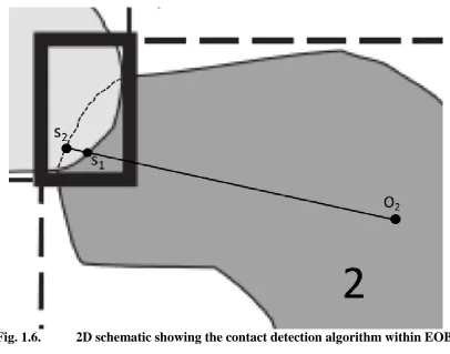
Fig. 1.6. 2D schematic showing the contact detection algorithm within EOB.
A quick check for overlap is first performed along the line connecting the center of the two particles as shown in Fig. 2.5 to save computational cost. If there is no overlap along the line of centers and an EOB has been detected, the surface of particle 1 is scanned with a resolution of Nbox within the EOB and checked if the surface points are
within the EOB. Though not very intuitive, it is possible that some part of the surface of the particles within the angle range of the EOB is outside the box and those points do not need to checked for overlap since it is not possible for those points to be overlapping the other particle. From each surface point on particle 1 which is inside the EOB, an
imaginary line segment is drawn to the center of particle 2 (S1O2 in Fig. 1.6). Now the
line segment is extended to the surface of particle 2 (S2O2 in Fig. 1.6). If S1O2 is less than
method is purely a geometrical solution and does not rely on numerical iteration schemes, which are more straightforward and elegant.
Another significant recent development to the method for mathematically representing irregular shaped particles using spherical harmonic expansions is the
addition of the uniform thickness shell to the particles (Garboczi and Bullard, 2013). This feature has several important applications such as the ability to model the interfacial transition zone (ITZ) found in concrete. The uniform thickness shell for a sphere is
straightforward to imagine and to determine mathematically. For any given angle (𝜃𝑖, 𝜙𝑖), the radius of the uniform thickness shell is just the sum of the radius vector of the original sphere r(𝜃𝑖, 𝜙𝑖) and the thickness vector t(𝜃𝑖, 𝜙𝑖), since the thickness vector is always parallel to the surface normal of the sphere. However, even for shapes such as ellipsoids, the radius vector may not be parallel to the surface normal vector. Hence, a numerical method to determine the extension to the radius vectors was developed (Garboczi and Bullard, 2013) such that the thickness vector normal to any surface point can be a
1.3Research Objectives
The EOB method and the uniform thickness shell method are two recently developed algorithms (Garboczi and Bullard, 2013) for the spherical harmonic
representation of irregular shapes. It is identified that the integration of the EOB method to detect contact can potentially improve the performance of generating the Anm model. The ability to add uniform thickness shells to particles in the Anm model can be used to control the minimum inter-particle distance between particles by not allowing the uniform thickness shells to overlap. If the purpose of the uniform thickness shell is to control the inter-particle distance, the final model should not contain the actual shells. However, allowing the uniform thickness shell to overlap other shells and particles increases the applicability of the Anm model. One implication of adding this capability to the Anm model is that the shell also becomes part of the output data and hence data visualization will be affected. It was identified that data parallelism can be introduced into the Anm model to allow the program to take advantage of the threaded, multi-core processors available on most computers today and speed up the particle packing algorithm.
The objectives of this research can be summarized as follows:
(1) Integrate the EOB method into the Anm model and perform a quantitative study of the performance improvements.
(3) Identify performance bottlenecks in the code, implement shared-memory parallelism in the code and study the performance improvement gained by adding parallelism to the code.
(4) Introduce the ability to allow uniform thickness shells to overlap other
particles and shells and explore data visualization techniques for overlapping shells using a 2D slicing method.
(5) Characterize the wall effect observed in the Anm model using the 2D slicing method and quantify it using the radial distribution function (RDF).
Objectives (1) to (3) have been previously accomplished and are published in a journal article and presented in Chapter 2. Objective (4) and (5) are presented in Chapter 3. The conclusions of this research are drawn in Chapter 4 along with some thoughts on the outlook of this research for the future.
1.4 References
Amirjanov, A. and Sobolev, K. (2008) ‘Optimization of a Computer Simulation Model for Packing of Concrete Aggregates’, Particulate Science and Technology, 26(4), pp. 380–395. doi: 10.1080/02726350802084580.
Bentz, D. P. (1997) ‘Three-Dimensional Computer Simulation of Portland Cement Hydration and Microstructure Development’, Journal of the American Ceramic Society. Wiley Online Library, 80(1), pp. 3–21.
Bentz, D. P., Garboczi, E. J., Bullard, J. W., Ferraris, C., Martys, N. and Stutzman, P. E. (2006) ‘Virtual testing of cement and concrete’, in Significance of tests and properties of concrete and concrete-making materials. ASTM International. Bentz, D. P., Garboczi, E. J. and Snyder, K. A. (1999) A hard core/soft shell
microstructural model for studying percolation and transport in
Bullard, J. W. and Garboczi, E. J. (2006) ‘A model investigation of the influence of particle shape on portland cement hydration’, 36, pp. 1007–1015. doi: 10.1016/j.cemconres.2006.01.003.
Garboczi, E. J. (2002) ‘Three-dimensional mathematical analysis of particle shape using X-ray tomography and spherical harmonics: Application to aggregates used in concrete’, Cement and Concrete Research, 32(10), pp. 1621–1638. doi: 10.1016/S0008-8846(02)00836-0.
Garboczi, E. J. (2011) ‘Three dimensional shape analysis of JSC-1A simulated lunar regolith particles’, Powder Technology, 207(1–3), pp. 96–103. doi:
10.1016/j.powtec.2010.10.014.
Garboczi, E. J. and Bullard, J. W. (2013) ‘Contact function, uniform-thickness shell volume, and convexity measure for 3D star-shaped random particles’, Powder Technology. Elsevier B.V., 237, pp. 191–201. doi: 10.1016/j.powtec.2013.01.019. Haecker, C.-J., Garboczi, E. J., Bullard, J. W., Bohn, R. B., Sun, Z., Shah, S. P. and
Voigt, T. (2005) ‘Modeling the linear elastic properties of Portland cement paste’,
Cement and Concrete Research. Elsevier, 35(10), pp. 1948–1960.
Jackson, M. D., Ciancio Rossetto, P., Kosso, C. K., Buonfiglio, M. and Marra, F. (2011) ‘Building Materials of the Theatre of Marcellus, Rome*’, Archaeometry, 53(4), pp. 728–742. doi: 10.1111/j.1475-4754.2010.00570.x.
Masoero, E., Del Gado, E., Pellenq, R. J.-M., Yip, S. and Ulm, F.-J. (2014) ‘Nano-scale mechanics of colloidal C-S-H gels.’, Soft matter, 10(3), pp. 491–9. doi:
10.1039/c3sm51815a.
Pellenq, R. J.-M., Kushima, A., Shahsavari, R., Van Vliet, K. J., Buehler, M. J., Yip, S. and Ulm, F.-J. (2009) ‘A realistic molecular model of cement hydrates’,
Proceedings of the National Academy of Sciences. National Acad Sciences, 106(38), pp. 16102–16107.
Qian, Z., Garboczi, E. J., Ye, G. and Schlangen, E. (2014) ‘Anm: a geometrical model for the composite structure of mortar and concrete using real-shape particles’,
Materials and Structures. Available at:
http://link.springer.com/article/10.1617/s11527-014-0482-5 (Accessed: 24 January 2015).
Quiroga, P. and Fowler, D. (2004) ‘The effects of aggregates characteristics on the performance of Portland cement concrete’. Available at:
http://zanran_storage.s3.amazonaws.com/www.nssga.org/ContentPages/1117303 52.pdf (Accessed: 24 February 2014).
Scarborough, J. B. (1966) ‘Numerical Mathematical Analysis Johns Hopkins U’, Press, Baltimore, pp. 299–303.
CHAPTER TWO: IMPROVED MODEL FOR THREE-DIMENSIONAL VIRTUAL CONCRETE: ANM MODEL
This chapter is published by ASCE (American Society of Civil Engineers) in the Journal of Computing in Civil Engineering and is referenced below:
IMPROVED MODEL FOR THREE-DIMENSIONAL VIRTUAL CONCRETE: ANM MODEL
Stephen Thomas1
Yang Lu, Ph.D., M.ASCE2 E. J. Garboczi3
Published in:
Journal of Computing in Civil Engineering May 8,2015
1Graduate Research Assistant, Department of Materials Science & Engineering,
Boise State University, Boise, ID 83725, USA
2Assistant Professor, Department of Civil Engineering, Boise State University,
Boise, ID 83725, USA
3NIST Fellow, Applied Chemicals and Materials Division, National
Institute of Standards and Technology, 325 Broadway MS 647, Boulder, CO
Abstract
Construction aggregate particles, fine or coarse, can be scanned by X-ray
computed tomography and mathematically characterized using spherical harmonic series, and can then be used to simulate random parking of irregular aggregates to form a virtual mortar or concrete using the Anm model. Any other similar composite system of irregular (star-shaped) particles in a matrix can also be simulated. This paper integrates two new algorithms into the Anm model. The first new algorithm is the extent overlap box (EOB) method that detects interparticle contact, and the second is the capability of adding a uniform-thickness shell to each particle. Parameter analysis has shown that the EOB method leads to a more accurate detection of interparticle contact with a smaller computational cost than the previously used Newton-Raphson method. The uniform-thickness shell provides a customizable tool to control the minimum intersurface distance of particles during the parking process, as well as to simulate processes and
2.1 Introduction
Concrete is primarily composed of coarse aggregates, fine aggregates (sand), and cement paste. Software packages like the Virtual Cement and Concrete Testing
Laboratory (VCCTL) (Bentz et al. 2006; Bullard and Garboczi 2006) use computer-generated models to predict various properties of concrete. The accuracy of the models being used in the simulation plays an important role in predicting concrete behavior. Aggregate characteristics such as density and uniformity of aggregate packing and the corresponding particle size distribution (PSD) play a paramount role in strength and behavior of these concretes (Aïtcin 1998; Alexander and Mindess 2005; Neville 2011). Using realistic aggregate shapes instead of spheres (Amirjanov and Sobolev 2008) or ellipsoids can greatly improve the accuracy of such models in situations where aggregate shape is important, such as fresh concrete rheology, early-age mechanical properties, and fracture processes.
Aggregate shape and grading can significantly influence concrete workability (Koehler and Fowler 2007). Excessively flat and elongated aggregates typically have a lower packing density (PD) than more equiaxed aggregates, resulting in more paste being required to fill the voids between aggregates. There is a clear relationship between shape, texture, and grading of aggregates and the voids content of aggregates (Dewar 1999; De Larrard 1999). In fact, flaky, elongated, angular, and unfavorably graded particles lead to higher voids content than cubical, rounded, and well-graded particles. Further, these kinds of aggregates exhibit increased interparticle friction, resulting in reduced
normal aggregates. The proper selection of aggregates can minimize the water and cementitious materials contents needed to ensure adequate workability. Dense particle packing reduces paste consumption, thereby also providing significant cost savings (Kwan and Fung 2009; Kwan and Mora 2001). Models for predicting concrete compressive strength also base their validation on producing concrete mixtures of optimum packing density (Lecomte et al. 2005). An in-depth understanding of the packing of aggregates in concrete is therefore essential in optimizing the mix composition.
introduction of the method of using spherical harmonic series to represent and manipulate irregularly shaped particles (Garboczi 2002), it is possible to create more accurate models to simulate concrete microstructural behaviors and other complex particle systems.
The random shapes of real aggregate particles can be extracted using a
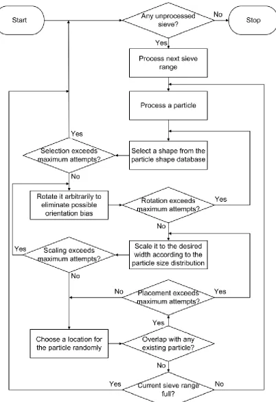
none of these attempts were successful in parking the particle from the current sieve, the next sieve is selected and this process is repeated. The Anm model can be used at several length scales. If the matrix is considered to be water, then the particles can be cement grains and the model represents fresh, fluid cement paste. If the matrix is cement paste, then the particles are sand grains and the model represents mortar, solid or fluid. If the matrix is considered to be mortar, then the particles are coarse aggregates and the model represents fluid or solid concrete.
When placing a particle, it is not very efficient, when there are more than a few particles, to search for overlap with all the previously parked particles in the entire
container. Therefore, the container is divided into equal parts along the length, width, and height where each section is called a bin. Using the dimensions of each particle and its center point, it is possible to determine the bins it touches. Because the particles touching those bins are known, only that subset of particles needs to be checked for overlap instead of all the particles in the simulation box. This method of reducing the search extent is also known as spatial decomposition and is extensively used in collision detection (Jiménez and Segura 2008) of geometric object such as complex polyhedra. Some of the methods that rely on hierarchical data structures based on recursive subdivision of space are Quadtrees in two dimensions, Octrees in three dimensions (Ayala et al. 1985), AABB trees (Bergen 1997), and sphere trees (Bradshaw and O’Sullivan 2004).
ranges add up to the total particle size distribution. In the Anm model, each sieve range volume must be occupied before placing particles from the next sieve range, starting from the largest sieve range.
Fig. 2.1. Placing star-shaped particles to model material mesostructure of mortar or concrete.
Fig. 2.1 is the visualization of the progress of particle packing in the container. In this illustration, three sieve ranges are assigned in the following order: 8 to 10 mm, 6 to 8 mm, and 2 to 6 mm. The particle dimension used in the sieve range is the particle width (Erdoğan et al. 2007). The length of a particle is defined as the longest point-to-point distance in the particle, and the width is defined the same way except that it must be perpendicular to the length. Each sieve range is denoted by a parking group [parking is a synonym for placement (Cooper 1988), so there are three parking groups for this
algorithm will go on to the next size group (middle size particles), which will be selected and parked in the same manner. This procedure will be repeated until the final attempt has been finished for the particles belonging to the smallest size parking group. The Anm model allows placement of the particles according to either periodic or nonperiodic boundary conditions. In nonperiodic boundary conditions, no particles are allowed to extend beyond or even touch the sides of the unit cell, whereas when using periodic boundary conditions particles that would extend beyond a unit cell boundary are allowed and are checked against contact in the periodic direction. Ghost particles are created whenever a particle is placed that has some portion extending beyond the unit cell boundary (Qian 2012; Qian et al. 2014)
harmonic series representation. Such surface zones occur in many kinds of composite particle systems, so this algorithm, integrated into the Anm model, should have general utility. Henceforth, this uniform-thickness shell shall simply be referred to as shell in this paper. In addition, the ability to place shells around each particle means that the
Euclidean distance from each particle’s surface at every point of the surface can be known so that processes that are a function of distance from a particle surface can be more easily simulated.
In addition to the shell algorithm, two other important improvements to the Anm model, described and used in this paper, are establishing a new, faster, and more accurate particle contact algorithm, and adding a degree of parallelism into the Anm code so that it runs much faster than the original model (Qian 2012; Qian et al. 2014). Recently, the Anm model has been used to create high quality three-dimensional tetrahedral mesh (Lu and Garboczi 2014), demonstrating its applicability in microstructural corrosion
modeling using finite-element analysis. The meshing method converts the 3D multiphase microstructure surface geometry created by the Anm model into a tetrahedral mesh without sacrificing the shape features.
The rest of this paper attempts to study the effects of using the new particle contact method and shell in the concrete mesostructure model. “Integration of New Search Algorithm” discusses integration of the new contact function into the Anm model. The method of adding a shell to the irregularly shaped particles is discussed in
Discussion” illustrates some results obtained with the improved Anm model.
“Conclusions and Future Research” concludes the discussions and projects the direction of future research.
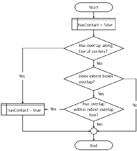
2.2 Integration of New Search Algorithm
Fig. 2.2. Three-step algorithm for searching contact.
the third step.
Fig. 2.3. Two particles with minimal overlap.
Fig. 2.5. Schematic representation of two particles which do not overlap along the line of center points in 2 dimensions, but have a non-zero volume EOB.
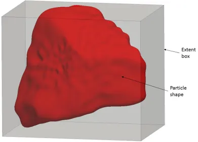
Fig. 2.6. Extent box for an irregular shaped particle.
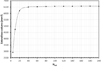
dimension of the extent box (Vbox) was observed as the value of Next was increased
(Garboczi and Bullard 2013).
If the extent boxes of two particles do not overlap each other, there is zero probability that the particles also overlap each other. But, if the two extent boxes do overlap, then the particles themselves can overlap only within the intersection of the extent boxes, which is itself a rectangular box called the EOB. The EOB is the only volume that needs be considered further to determine overlap or nonoverlap.
Fig. 2.8. A two-dimensional illustration of the Doverlap with respect to two
overlapping irregular shaped particles.
When two particles are found to have a nonzero volume EOB, the minimum and maximum values of θ and ∅ within the overlap box for each particle are determined. Then the surface points of the particle along those directions are scanned to check if any of those points are overlapped by the second particle. The accuracy and speed of this measurement is controlled using a parameter Nbox, which is the number of surface points
scanned along the range of each of these angles. Fig. 2.7 illustrates how Nbox affects the
contact search algorithm in a two-dimensional layout (considering only θ unlike the actual three-dimensional case with θ and ∅). Here because Nbox is equal to 5 between
angles θ1 and θ2, only five surface points are checked for contact. If the value of Nbox is
of Nbox increases, the scan becomes finer but computationally more expensive. So, the
value of Nbox determines the balance between the efficiency and the accuracy of this
search. More quantitatively, the optimum value of Nbox can be calculated by studying the
maximum distance, denoted Doverlap, between the surfaces of the overlapped particles in
any direction from the center of one of the particles. This distance is schematically
represented in Fig. 2.8. For two particles with no overlap, the value of Doverlap will be zero
for any value of Nbox. But for two overlapping particles, Doverlap will have a nonzero value
that is dependent on the value of Nbox. Once the value of Nbox is large enough, the value
of Doverlap does not change any more. A further increase in the value of Nbox will not be
useful because it will not increase the accuracy of the overlap determination.
More detailed analysis in “Results and Discussion” of the two barely overlapping particles shown in Fig. 2.3 will serve to describe the optimum values found for Next and
Nbox.
The EOB contact algorithm (Garboczi and Bullard 2013) is then faster than the Newton Raphson method (Qian, 2012;Qian et al., 2014) because only the surface points on one particle that are also inside the EOB are checked for contact with the other particle. It is also more accurate than the Newton Raphson method because false negatives were not seen in an extensive series of visual checks.
2.3 Integration of the Uniform-Thickness Shell Algorithm into Anm
higher concentration of large voids and cracks in the ITZ was observed. It was noted that the connectivity of the weaker areas such as large voids and cracks along the interface governs failure.
Fig. 2.9. Adding a shell by increasing the length of the radius vector by different amounts at different original surface points.
Fig. 2.10. Illustration of the vector equation with three unknowns 𝜷, 𝜽′ 𝒂𝒏𝒅 ∅′.
The length of the radius extension can be calculated by solving the vector Eq. (2.1) illustrated in Fig. 2.10, where t is the thickness and the unknowns are β, θ’, and ∅’. The three equations and three unknowns give rise to a system of equations that can be solved using the Newton-Raphson method for each choice of θ and ∅ (Garboczi and Bullard 2013)
𝑟 (𝜃, ∅′) + 𝑡𝑛̂(𝜃′, ∅′) = 𝑟 (𝜃, ∅) + 𝛽𝑟̂(𝜃, ∅) (2.1)
Fig. 2.11 shows a visualization of a shell around a single particle. The wired surface shows the shell, while the solid surface shows the original surface of the original irregularly shaped particle. Here particle length represents the largest surface-to-surface distance.
The volume fraction of the interfacial layer or shell in other types of composite materials can be a significant contributor to macroscopic physical properties (Xu et al. 2014b).
The shell model, along with the original Anm model, has the potential to serve as a microstructural modeling tool in several areas of research that are difficult to do
experimentally either due to the scale or due to the complexity of the materials. Two interesting studies that can benefit from this are the effects of ITZ on the electrical conductivity of mortar (Shane et al. 2000) and interfacial structures that have been found to have a significant effect on thermal conductivity of nanoparticle-fluid mixtures (Xie et al. 2005). More recently, the effect of ITZ on the diffusivity of chlorine in cementitious materials were also studied (Lu et al. 2012). In the chlorine diffusion research, the Anm model was employed to build a virtual mortar microstructure and a small surface crack was created on top of it to study the influence of crack on chlorine transport. The 3D multiphase microstructure meshing method (Lu and Garboczi 2014) was used to create 3D tetrahedral elements. The created 3D mesh was included in finite-element analysis for chlorine diffusion simulation.
2.4 Parallel Optimization of Anm Code for Faster Execution
The average CPU utilization of the test program was measured to be 12.4% ≈ 1=8. A typical pseudocode in such programs is shown in Fig. 2.12.
Fig. 2.12. Pseudo code for a typical serial code containing time consuming loops.
Fig. 2.13. Pseudo code for time consuming loops after parallelization.
The sequential code is not utilizing the maximum capacity of the multicore system. Parallel programming techniques can be used to allow the independent iterations to execute in parallel, utilizing the processors that are otherwise idle. For the purpose of this study, the authors chose to use the Microsoft Parallel Patterns Library (PPL) (Gebali 2011) to enable parallel execution of the code. The PPL library provides “parallel_for”
constructs, which can be used to replace normal “for” loops to easily achieve parallel
Significant improvements were observed in the execution of the test program after incorporating the PPL. The test program now had an average CPU utilization of 87.9%. This improvement in performance is achieved by distributing tasks within the
independent iterations in the pseudocode among many threads generated by the operating system. These threads have the ability to utilize the individual processors of the CPU concurrently. For instance, the algorithm for rotating particles in the Anm model concurrently manipulates surface points along the azimuthal angle (θ) in random order unlike a sequential code where the surface points will be manipulated sequentially along angles 0 to π. In this function, the Anm data representing a single particle shape are manipulated concurrently using multiple processors to achieve its rotation. Apart from the particle rotate function, similar parallelism has been implemented to the particle contact algorithm and uniform-thickness shell algorithm. Two types of parallelism can be achieved using the parallel libraries, namely, data parallelism and task parallelism. The method used in the Anm model as explained previously is an example of data parallelism and requires only minimal change from the sequential code. Task parallelism, on the other hand, is more effective in saving time but involves domain decomposition and distributive processing of task on different processors or computers (Subhlok et al. 1993). Therefore, introducing task parallelism requires more rigorous examination of the
algorithm and redesign of the code, so is a good opportunity for further development. 2.5 Results and Discussion
2.5.1 Particle-Particle Contact Function
The EOB method with parallelization (with eight processors) was found to be approximately 82% faster than the NR method (single processor). The simulation performed for this comparison packed particles from a coarse aggregate shape database into a cubic container of length 66 mm. The particle sizes were uniformly distributed from 7 to 11 mm. During the parking process, the authors recorded the time taken to check the overlap of 139 particle pairs for which the functions being compared were executed. A software timer was used to measure the time taken exclusively by the interparticle contact functions and the values were saved on a file by the program for analysis. The standard deviation of the execution time for the EOB method and NR method were 909 and 5,487 ms, respectively. The average execution times were 775 and 4,354 ms, respectively.
Fig. 2.15. The value of Doverlap increases as the value of Nbox increases for two particles
with minimal overlap. The value of Next was fixed at 80 for this measurement.
The efficiency of the EOB method depends on two key parameters, Next and Nbox.
As explained in “Integration of New Search Algorithm,” the optimum values for these parameters have been found by performing a parameter analysis. It can be seen in Fig. 2.14 that for values of Next > 40 there is very little change in the extent box volume. For
values of Next < 40, the extent box volume still varies significantly with the value of Next.
It can also be seen in Fig. 2.15 that beyond Nbox ≈ 90, there is very little variation in the
value of Doverlap so that increasing the value Nbox beyond this point should not increase the
accuracy of the overlap calculation. Thus, it is reasonable to use Next = 40 and Nbox = 90
for the given sample particle database. With the optimum values of Next and Nbox used,
structure of the spherical harmonic representation means that these values do not vary much across an aggregate type.
2.5.2 Uniform-Thickness Shell
The shell algorithm in “Integration of the Uniform-Thickness Shell Algorithm in Anm” considers only small values of shell thickness, t, so that there is no shell-shell or shell-particle overlap between the shell and the particle (Garboczi and Bullard 2013) when computing the shell for each particle. These kinds of overlaps introduce numerical instabilities. The authors have found that the thickness of a single shell, t, should be limited to 0.1% of the particle length to avoid this condition in the specific case of the several kinds of coarse aggregates studied so far. Parameter analysis has been performed with shell thickness from 0.1 to 2% of particle length. If a thick shell is desired, it is also more numerically stable to sequentially add several thin shells rather than using a single thick shell.
An interesting question discussed earlier (Garboczi and Bullard 2013) was if there was any difference in creating a single shell of thickness 5t or five shells of thickness t. Shells were added to a particle, first as a single shell of 0.1% thickness, then 10 shells with 0.01% thickness each, and finally 100 shells with 0.001% thickness relative to the particle length. The authors observed that the volume of the new particle remains the same. The overall time taken to create the uniform thickness increased approximately linearly because a similar shell generation algorithm is repeated more times for the larger number of shells.
Table 2.1 Particle size distribution and achieved volume fraction by particles from individual sieves
Shell thickness (%) Sieve 1 (10-11mm) Sieve 2 (9-10 mm) Sieve 3 (8-9 mm) Sieve 4 (7-8 mm) Total PD
0 0.2569 0.2540 0.2519 0.2524 0.2632
0.2 0.2569 0.2522 0.2503 0.2504 0.2619
0.4 0.2569 0.2523 0.2511 0.2514 0.2623
0.6 0.2575 0.2538 0.2530 0.2503 0.2631
0.8 0.2575 0.2538 0.2523 0.2416 0.2607
1 0.2505 0.2532 0.2524 0.2136 0.2514
1.2 0.2503 0.2507 0.2526 0.2473 0.2595
1.4 0.2503 0.2513 0.2525 0.1758 0.2411
1.6 0.2503 0.2521 0.2521 0.2081 0.2496
1.8 0.2501 0.2511 0.2511 0.2122 0.2501
2 0.2501 0.2520 0.2514 0.1952 0.2460
Table 2.2. Number of particles per sieve with respect to the change in shell thickness of the individual particles.
Shell thickness (%) Sieve 1 (10-11mm) Sieve 2 (9-10 mm) Sieve 3 (8-9 mm) Sieve 4 (7-8 mm) Total
0 50 67 89 126 332
0.2 50 66 89 126 331
0.4 50 66 91 125 332
0.6 50 66 88 127 331
0.8 50 66 89 124 329
1 49 66 91 110 316
1.2 49 65 89 125 328
1.4 49 65 90 91 295
1.6 49 65 89 107 310
1.8 49 66 90 110 315
2 49 66 90 100 305
In this simulation, there are other factors influencing the packing of the particles. The random packing does not result in a reliable dense packing where all the particles are almost touching their neighbors. Without the shell, many particles are already parked separately by a distance larger than the thin shell. Therefore, only a fraction of the
Sieve 4, for shell thickness of 1.2 and 1.6%. Table 2.2 shows the actual number of particles parked from each sieve.
Fig. 2.16. Illustration of the (a) decreasing trend in PD and (b) number of particles packed with the increase in shell thickness.
Fig. 2.17. Illustration of the linear increase in shell volume fraction with the increase in shell thickness.
particular study. The total shell volume fraction increases. The overall packing density has a close correlation with the total number of particles packed. It is also observed that the volume fraction of the shell increased by ∼4.5%, the achieved PD dropped by ∼6.5%, and the total number of particles dropped ∼8% as the shell thickness is increased from 0 to 2% of the individual particle length. Overall, the addition of shell will affect the PD. With the increase of the shell thickness, the PD will be reduced. The thicker the shell, the less particles can be packed.
2.5.3 Effect of Random Locations on Packing Density and Particle Size Distribution In the Anm model, there are four internal particle placement parameters: the number of random locations attempted, the number of random orientations attempted, the number of particle widths in a given sieve range attempted, and the number of random shapes.
In the Anm model, a particle with a specific shape, orientation, and width is selected and an attempt is made to place it at a random location within the container. If this attempt fails because of an overlap with another parked particle, a different random location is chosen within the container and an attempt is made to place it again. However, this cannot be done indefinitely. So, a maximum number of random locations are
attempted before trying to use another random particle shape, width, or orientation. These are parameters for the maximum number of shapes, widths, and orientations allowed, thus it can be said that there are four sources of randomness in this algorithm. In
experience. Additionally, its low computational cost allows the use of many random trials with- out unreasonably increasing the execution time. In the following study, coarse aggregate shapes ranging from 4.75 to 11 mm were packed in decreasing order of size in a cubic container having an edge length of 66 mm. The intended value of the PD was 0.355. Similar to the study that resulted in Table 2.1 and 2.2, the random locations parameter was varied while keeping the other random parameters fixed.
Table 2.3. Changes in PD and PSD of the Anm model as the number of random locations attempted for each particle is increased.
No. of random locations No. of particles packed Achieved PD Sieve 1 10 mm to
11 mm (0.18)
Sieve 2 9 mm to
10 mm (0.18)
Sieve 3 8 mm to
9 mm (0.18)
Sieve 4 7 mm to
8 mm (0.18) Sieve 5 6 mm to7mm (0.18) Sieve 6 4.75 mm to 6 mm (0.10)
30 380 0.207 0.183 0.174 0.054 0.064 0.018 0.087
60 392 0.220 0.183 0.129 0.119 0.082 0.040 0.065
90 354 0.214 0.183 0.129 0.182 0.026 0.018 0.063
120 340 0.230 0.183 0.181 0.134 0.050 0.084 0.014
140 348 0.240 0.183 0.181 0.180 0.028 0.092 0.010
285 416 0.249 0.183 0.181 0.183 0.066 0.018 0.069
450 426 0.255 0.183 0.181 0.183 0.066 0.042 0.063
975 450 0.281 0.183 0.181 0.183 0.123 0.098 0.023
1500 510 0.295 0.183 0.181 0.183 0.174 0.042 0.068
In Table 2.3, contrary to intuition, the PD is reduced when the locations attempts were increased from 60 to 90. This phenomenon can be understood by analyzing the individual PD of Sieve 3. While attempting to pack the particles with 90 locations, Sieve 1 and 2 particles packed exactly the same amount as that of 60 locations. But Sieve 3 particles benefited from the increased number of attempted random locations and packed better. These particles filled up a significant amount of empty space, leaving the
the number of random locations are increased to 140, 450, and 1,500. However, the overall PD does not decrease for these cases, as was seen when going from 60 to 90 placement attempts, due to the smaller particle sizes (Sieves 4, 5, and 6) affected. The periodic packing method seems to generate a slightly denser packing compared with the nonperiodic packing method, which is expected because more efficient use would be made of regions near the edge of the cell when employing periodic boundary conditions. As the random location attempts were increased, it was observed that the larger particles, which are parked first, began to pack more densely and achieve the suggested volume fraction for their sieve range. The smaller particles, which are parked last, may require a larger number of random location attempts to reach their suggested volume fraction for each sieve due to higher PD of the particles from the prior sieves. Currently, all the sieves are assigned the same number of random location attempts and this value is usually a large value suitable for the last sieve being used. This raises a reasonable question about the possibility of using a different number of random locations for different sieves such that the last sieve is entitled to many more attempts than the first sieve. However, the program stops parking particles from a sieve when either the maximum number of
2.5.4 Performance Comparison
This section compares the performance of serial processing to the parallel computing achieved using the PPL. The most time-consuming loops were identified in the existing program and were upgraded with the PPL. Figs. 2.18 and 2.19 show the comparative time (in milliseconds) taken to execute two different functions in serial and parallel. Fig. 2.18 indicates the comparison of time taken to rotate a particle using serial and parallel execution of the algorithm. The parallel version has accelerated the particle manipulation operations significantly.
Fig. 2.19. Comparison of the EOB contact searching algorithm using serial and parallel execution (8 processors).
Fig. 2.19 shows comparison of the EOB contact searching algorithm using serial and parallel execution. The large variations of serial run time shown in Fig. 2.19 can be attributed to the fact that as the extent of the overlap between the two particles in question decreases, the overlap detection requires more computation time. The parallel contact function reduces the computational load to some extent by randomly scanning points on the extent overlap box. This random scanning process has a higher probability of finding an overlap faster when compared with the sequential and ordered scan in the serial code. Apart from this advantage, the parallel code utilizes multiple processors available to process the data, thereby reducing computational load.
which a program is designed to be executed in parallel. The speedup parameter is defined by Eq. (2.2)
𝑆𝑝(𝑛) =
𝑇∗ (𝑛) 𝑇𝑝(𝑛)
(2.2)
where Sp(n) = speedup; T*(n) = execution time of the best sequential
implementation to solve the same problem of size n; and Tp(n) = execution time of the
parallel execution using p processors. Linear speedup is achieved when
𝑆𝑝(𝑛) = 𝑝 . (2.3)
Efficiency is given by
𝐸𝑝(𝑛) = 𝑆𝑝(𝑛)
𝑝 . (2.4)
Ideal speedup Sp(n) = p corresponds to an efficiency of
𝐸𝑝(𝑛) = 1 . (2.5)
Fig. 2.20. Efficiency of contact searching algorithm where the number of participating processors p=8.
results shown in Fig. 2.20 indicate that a speedup of around 5 and an efficiency of close to 0.6 was achieved with the current parallel mechanism. This is a substantial
improvement in performance compared with the sequential execution with a minimal amount of change in the code. The improvement in performance is not linear because only data parallelization has been implemented in the current version. Examples for data parallelism include the individual particle rotation function and two-particle contact function using the EOB method. However, there are other parts of the code, such as the particle parking function that parks one particle at a time sequentially. Parallelizing this function using task parallelism techniques such as message passing interface (MPI) is expected to produce a nearly linear performance improvement.
2.6 Conclusions and Future Research
Particle size distribution effects have been studied and standardized in ASTM standards (Lamond and Pielert 2006), but particle shape effects have not been extensively studied because of their complexity. The Anm model provides an effective method to simulate the proportioning of the aggregates considering real particle shape effects in concrete. The microstructure of mortar and concrete, or indeed any such composite material that can be modelled by star-shaped particles embedded in a matrix, can be simulated using the Anm model, which has been greatly improved and augmented. The following conclusions are made based on the results presented here:
• The EOB method is more efficient and accurate for the detection of interparticle contact when compared with the NR method used by the first version of the Anm model. • The uniform-thickness shell provides a customizable tool to control the minimum
valuable method to simulate the highly heterogeneous properties of an interfacial transition zone around the particles. The two main factors that determine the effect of the nonoverlapping shells on achieved PD is the shell thickness t and the number of attempts to place the particles at random locations.
• Using the parallel processing application programming interface (API) framework, a speedup of approximately 5 and an efficiency close to 0.6 was achieved with the current parallel mechanism. This is a substantial improvement in performance compared with sequential execution using only a minimal amount of code change.
Future research will focus on more efficient parking methods that need to be devised to create more realistic models of the concrete microstructure, especially if size scales, like those between fine and coarse aggregate in concrete, are to be mixed. Task parallelization in addition to the present data parallelization will be studied. One of the focus areas will be to improve the parking density so that more realistically dense systems can be generated and studied. Applications will be generated as well as
continually improving the Anm model, such as developing a new shell algorithm that has the ability to add shells of larger volumes.
2.7 Author Justifications
The research presented in this justification was a collaborative effort by Stephen Thomas, Dr. Yang Lu and Dr. E. J. Garboczi. Stephen took the responsibility of the lead author since he had the responsibility of preparing the code, testing it, performing the simulations and manuscript writing. Dr. Lu and Dr. Garboczi contributed to the research with detailed discussions and in-depth constructive feedback during the code
research contribution was a partial fulfilment of the requirements for a Master of Science degree in Materials Science and Engineering at Boise State under the advisement of Dr. Yang Lu.
2.8 References
Aïtcin, P.-C. (1998). High-performance concrete, E&FN Spon, NewYork.
Alexander, M. G., and Mindess, S. (2005). Aggregates in concrete, Taylor & Francis, New York.
Amirjanov, A., and Sobolev, K. (2008). “Optimization of a computer sim- ulation model for packing of concrete aggregates.” Part. Sci. Technol., 26(4), 380–395.
Arfken, G. B. (1970). Mathematical methods for physicists, Academic, New York. Ayala, D., Brunet, P., Juan, R., and Navazo, I. (1985). “Object representation by means
of nonminimal division quadtrees and octrees.” ACM Trans. Graph., 4(1), 41–59. Bentur, A., Alexander, M. G., and Comm, R. T. (2000). “A review of the work of the
RILEM TC 159-ETC: Engineering of the interfacial transition zone in cementitious composites.” Mater. Struct., 33(2), 82–87.
Bentz, D. P., Garboczi, E. J., Bullard, J.W., Ferraris, C. F., and Martys, N. S. (2006). “Virtual testing of cement and concrete.” Significance of tests and properties of concrete and concrete-making materials, J. Lamond and J. Pielert, eds., ASTM, West Conshohocken, PA.
Bergen, G. V. D. (1997). “Efficient collision detection of complex deformable models using AABB trees.” J. Graph. Tools, 2(4), 1–13.
Boon, C. W., Houlsby, G. T., and Utili, S. (2012). “A new algorithm for contact detection between convex polygonal and polyhedral particles in the discrete element
method.” Comput. Geotech., 44, 73–82.
Bullard, J. W., and Garboczi, E. J. (2006). “A model investigation of the influence of particle shape on portland cement hydration.” Cem. Concr. Res., 36(6), 1007– 1015.
Cooper, D. W. (1988). “Random-sequential-packing simulations in three dimensions for spheres.” Physical Rev. A, 38(1), 522–524.
De Larrard, F. (1999). Concrete mixture proportioning: A scientific approach, CRC Press.
Dewar, J. D. (1999). Computer modelling of concrete mixtures, E & FN Spon, New York.
Erdoğan, S. T., Garboczi, E. J., and Fowler, D.W. (2007). “Shape and size of microfine aggregates: X-ray microcomputed tomography vs. laser diffraction.” Powder Technol., 177(2), 53–63.
Garboczi, E. J. (2002). “Three-dimensional mathematical analysis of particle shape using X-ray tomography and spherical harmonics: Application to aggregates used in concrete.” Cem. Concr. Res., 32(10), 1621–1638.
Garboczi, E. J., and Bullard, J. W. (2013). “Contact function, uniform- thickness shell volume, and convexity measure for 3D star-shaped random particles.” Powder Technol., 237, 191–201.
Garboczi, E. J., Cheok, G. S., and Stone,W. C. (2006). “Using LADAR to characterize the 3-D shape of aggregates: Preliminary results.” Cem. Concr. Res., 36(6), 1072– 1075.
Gebali, F. (2011). “Algorithms and parallel computing.” Wiley, Hoboken, NJ. Goldasteh, I., Ahmadi, G., and Ferro, A. (2012). “A model for removal of compact,
rough, irregularly shaped particles from surfaces in turbulent flows.” J. Adhes., 88(9), 766–786.
Koehler, E. P., and Fowler, D. W. (2007). Role of aggregates in self- consolidating concrete, International Center for Aggregates Research, Austin, TX.
Kwan, A. K. H., and Fung,W.W. S. (2009). “Packing density measurement and
modelling of fine aggregate and mortar.” Cem. Concr. Compos., 31(6), 349–357. Kwan, A. K. H., and Mora, C. F. (2001). “Effects of various shape parameters on packing
of aggregate particles.” Mag. Concr. Res., 53(2), 91–100.
Lamond, J. F., and Pielert, J. H. (2006). Significance of tests and properties of concrete and concrete-making materials, ASTM, West Conshohocken, PA.
Lecomte, A., de Larrard, F., and Mechling, J. M. (2005). “Predicting the compressive strength of concrete: The effect of bleeding.” Mag. Concr. Res., 57(2), 73–86. Lu, Y., and Garboczi, E. (2014). “Bridging the gap between random micro- structure and
3D meshing.” J. Comput. Civ. Eng., 10.1061/(ASCE)CP .1943-5487.0000270, 04014007.
Lu, Y., Garboczi, E., Bentz, D., and Davis, J. (2012). “Modeling chloride transport in cracked concrete : A 3-D image-based microstructure simulation.” COMSOL Conf. 2012, Boston.
Max, N. L., and Getzoff, E. D. (1988). “Spherical harmonic molecular surfaces.” IEEE Comput. Graph. Appl., 8(4), 42–50.
Mondal, P., Shah, S. P., and Marks, L. D. (2009). “Nanomechanical properties of interfacial transition zone in concrete.” Nanotechnology in construction, Z. Bittnar, P. M. Bartos, J. Němeček, V. Šmilauer, and J. Zeman, eds., Springer, Berlin, 315–320.
Neville, A. M. (2011). Properties of concrete, Pearson, New York.
Ollivier, J. P., Maso, J. C., and Bourdette, B. (1995). “Interfacial transition zone in concrete.” Adv. Cem. Based Mater., 2(1), 30–38.
Qian, Z., Garboczi, E. J., Ye, G., and Schlangen, E. (2014). “Anm: A geometrical model for the composite structure of mortar and concrete using real-shape particles.” Mater. Struct., in press.
Rauber, T. R. G. (2010). Parallel programming: for multicore and cluster systems, Springer, Berlin.
Shane, J. D., Mason, T. O., Jennings, H. M., Garboczi, E. J., and Bentz, D. P. (2000). “Effect of the interfacial transition zone on the conductivity of portland cement mortars.” J. Am. Ceram. Soc., 83(5), 1137–1144.
Sobolev, K., and Amirjanov, A. (2004). “The development of a simulation model of the dense packing of large particulate assemblies.” Powder Technol., 141(1–2), 155– 160.
Subhlok, J., Stichnoth, J. M., O’hallaron, D. R., and Gross, T. (1993). “Exploiting task and data parallelism on a multicomputer.” ACM SIGPLAN Notices, 28(7), 13– 22.
Xie, H. Q., Fujii, M., and Zhang, X. (2005). “Effect of interfacial nanolayer on the effective thermal conductivity of nanoparticle-fluid mixture.” Int. J. Heat Mass Transfer, 48(14), 2926–2932.
Xu, W., Chen, W., Chen, H., Tian, X., and Zhao, H. (2014a). “Determination of
overlapping degree of interfacial layers around polydisperse ellipsoidal particles in particulate composites.” Phys. A Stat. Mech. Appl., 399, 126–136.