Spatial change detection using normal distributions transform

RESEARCH ARTICLE

Spatial change detection using normal

distributions transform

Ukyo Katsura

, Kohei Matsumoto

, Akihiro Kawamura

, Tomohide Ishigami

, Tsukasa Okada

and Ryo Kurazume

Abstract

Spatial change detection is a fundamental technique for finding the differences between two or more pieces of geometrical information. This technique is critical in some robotic applications, such as search and rescue, security, and surveillance. In these applications, it is desirable to find the differences quickly and robustly. The present paper proposes a fast and robust spatial change detection technique for a mobile robot using an on-board range sensors and a highly precise 3D map created by a 3D laser scanner. This technique first converts point clouds in a map and measured data to grid data (ND voxels) using normal distributions transform. The voxels in the map and the measured data are then compared according to the features of the ND voxels. Three techniques are introduced to make the proposed system robust for noise, that is, classification of point distribution, overlapping of voxels, and voting using consecutive sensing. The present paper shows the results of indoor and outdoor experiments using an RGB-D camera and an omni-directional laser scanner mounted on a mobile robot to confirm the performance of the proposed technique.

Keywords: Change detection, Laser scanner, RGB-D camera, Normal distributions transform

© The Author(s) 2019. This article is licensed under a Creative Commons Attribution 4.0 International License, which permits use, sharing, adaptation, distribution and reproduction in any medium or format, as long as you give appropriate credit to the original author(s) and the source, provide a link to the Creative Commons licence, and indicate if changes were made. The images or other third party material in this article are included in the article’s Creative Commons licence, unless indicated otherwise in a credit line to the material. If material is not included in the article’s Creative Commons licence and your intended use is not permitted by statutory regulation or exceeds the permitted use, you will need to obtain permission directly from the copyright holder. To view a copy of this licence, visit http://creat iveco mmons .org/licen ses/by/4.0/.

Introduction

Spatial change detection is a fundamental technique for finding the differences between two or more pieces of geometrical information. This technique is indispensa-ble in several applications, such as topographic change detection in airborne laser scanning [1, 2] or terrestrial laser scanning [3, 4], map maintenance in urban areas [5], preservation of cultural heritage [6], and analysis of plant growth [7]. In robotics, the detection of spatial changes around a robot is often used in some applications, such as daily service, search and rescue, security, and sur-veillance. For example, service robots, such as cleaning robots or delivery robots, which are used on a daily basis, require the ability of spatial change detection in order to safely and efficiently co-exist with humans, because

the environment can change dynamically according to human behavior. For these service robots, precise locali-zation is also required in order to perform a desired task. To improve the accuracy of the localization, spatial change detection is also important. For example, when using scan matching (or ICP) for localization in an envi-ronment where spatial changes exist, some points meas-ured by an on-board range sensor are different from the points in the map created previously. In this case, these points caused by the spatial changes should be detected and removed before applying scan matching.

In our previous paper [8], we proposed a fast spa-tial change detection technique by comparing 3D range data obtained by an on-board RGB-D camera (Kinect for Xbox One) and a high-precision 3D map created by a 3D laser scanner. This technique first converts point clouds in the map and measured data to grid data [normal distri-butions (ND) voxels] by normal distridistri-butions transform (NDT) [9], and classifies the voxels into three categories. The voxels in the map and the measured data are then

Open Access

*Correspondence: [email protected]

1 _{Kyushu University, 744 Motooka, Nishi-ku, Fukuoka-shi, Fukuoka}

819-0395, Japan

compared according to the category and features of ND voxels. Overlapping and voting techniques are also intro-duced in order to detect spatial changes more robustly. We conducted the preliminary experiments using a mobile robot equipped with a RGB-D camera in order to confirm the performance of the proposed spatial change detection techniques mainly in an indoor environment.

The present paper shows the experimental results of on-line localization and spatial change detection tech-niques mainly in outdoor environment using an omni-directional laser scanner (Velodybe HDL-32e). We also show the additional results of indoor experiments using an on-board RGB-D camera (Kinect for Xbox One). In the following sections, we firstly introduce the fast spatial change detection technique proposed in [8], and show the system settings. In addition, we conduct experiments in indoor and outdoor environments and compare the performance quantitatively with cutting-edge techniques.

Related research

Spatial change detection is a critical problem in some robotic applications [10–16]. Andreasson et al. [10] pro-posed autonomous change detection for a security patrol robot. They used color and depth information obtained from a 3D laser range finder and a camera. A precise ref-erence model was first created from multiple color and depth images and was registered by 3D normal distri-butions transform (3D-NDT) [17] representation. Spa-tial changes are detected by calculating the probabilistic value of the current point being different from the refer-ence model using the 3D-NDT representation and color information. Saarinen et al. [18] proposed Normal Distri-butions Transform Occupancy Maps (NDT-OM), which concurrently represent the occupancy probability and the shape distribution of points (NDT) in each voxel. The occupancy probability is calculated from a sensor model and the point distribution in the voxel, and the similarity measure of two NDT-OMs is defined by L2 distance

func-tion. Nùüez et al. [11] proposed a fast change detection technique using a mixture Gaussian model and a fast and robust matching algorithm. Point-based comparison of an environmental model and a large number of point cloud data measured by an on-board range sensor requires a large calculation cost. In order to solve this problem, they represented the environmental model and the meas-ured data with a mixture Gaussian model and processed the difference calculation using a high-speed algorithm. Fehr et al. [14] presents a 3D reconstruction technique of dynamic scenes involving movable objects using the trun-cated signed distance function (TSDF). They represented the current scene with TSDF grids and compared them with previous TSDF grids to obtain segmented movable objects in the scene. Luft et al. [15] proposed a stochastic

approach to evaluate whether a grid is changed in time according to full-map posteriors represented by real-valued variables. Their technique enables consideration of the full-path information of the laser measurement, as opposed to end-point based approaches. Moreover, it considers the confidence about the cell values as opposed to occupancy maps or a most-likely maps. [16]. Palazzolo et al. [16] proposed a fast spacial change detection tech-nique using a 3D model and a small number of 2D images. They assume a 3D model is given and spacial changes are detected using re-projection of 2D images without 3D reconstruction of the model.

In general, spatial change detection can be classified into three groups: point/mesh-based, height-based, and voxel-based comparisons. Point/mesh-based compari-son [6, 19] is a technique that compares the distance of nearest points or meshes in two point clouds, which is similar to the ICP algorithm [20]. Lague et  al. [4] pro-posed the use of the distance along normal direction of a local surface to make the algorithm robust to errors in 3D terrain data measured by a terrestrial laser scanner. In [3], point clouds are converted to panoramic distance images, which are compared directly. The problem with this technique is the degree to which the proper thresh-old is determined [19].

Height-based comparison is often used in geographi-cal analysis in earth sciences. The digital elevation map (DEM) of difference (DoD) is a popular technique to compare geographical data captured by airborne or ter-restrial laser scanners [2, 5, 21]. This technique also has the problem of selecting a proper threshold.

In voxel-based comparison, a point cloud is first con-verted to a voxel representation using, for example, an octree structure. Performing the XOR of occupancy vox-els is the simplest way [22] to find spatial differences. In [23], three metrics are compared in order to calculate the difference of voxels, which are the average distance, the plane orientation, and the Hausdorff distance. The Haus-dorff distance is the maximum value of the minimum distances of points in two voxels and indicates the best performance. However, the computational cost of the Hausdorff distance is quite high, because closest point pairs must be determined. In spatial change detection in 3D, not only point clouds but also a sequence of camera images has been used [24, 25].

spatial change detection, their technique can be classified as a point-based comparison because they used 3D-NDT to calculate the probability of a point being different from the reference model.

Scona et al. [26] presented the construction technique of a static map using a RGB-D camera. This method uti-lizes an energy function consisting of the errors in 2D images and the errors in the label assignment. Firstly the acquired color and depth images are segmented into several clusters, and the camera position and the label which indicates whether the current cluster belongs to a static object or not are determined simultaneously by minimizing the error function. A robust estimator using Cauchy penalty function is also adopted. In this method, the errors in color and depth images are simply defined as the difference of pixel values between the synthesized images from the map and the measured RGB-D data. In addition, the main purpose of the paper is to extract static objects to build a static map and not to detect newly appeared objects.

Fast 3D localization using NDT and a particle filter We have proposed an efficient 3D global localization and tracking technique for a mobile robot in a large-scale environment using 3D geometrical map and a RGB-D camera [27]. Conventional 3D localization techniques using 3D environmental information utilize a registration method based on point-to-point correspondence such as Iterative Closest Point (ICP) algorithm [28, 29], or voxel-to-voxel correspondence such as occupancy voxel count-ing [30]. However, these techniques are computationally expensive or low accuracy due to the costly nearest point calculation or the discrete voxel representation, and hard to be applied for a global localization using a large-scale environmental map. To tackle this problem, the proposed technique utilizes a ND voxel representation (Fig. 1) [28]. Firstly, a 3D geometrical map represented by point-clouds is converted to a number of ND voxels, and local features are extracted and stored as an environmental map. In addition, range data captured by a RGB-D cam-era is also converted to the ND voxels, and local features

are calculated. For global localization and tracking, the similarity of ND voxels between the environmental map and the sensory data is examined according to the local features, and optimum positions are determined in a framework of a particle filter.

Spatial change detection using ND voxels

In this section, we introduce a spatial change detection technique using ND voxels [8]. In “Fast 3D localization using NDT and a particle filter” section, the fast 3D local-ization using NDT and a particle filter is introduced [27]. The proposed spatial change detection technique re-uses the ND voxels generated and used for the proposed local-ization technique [27], and thus the computational cost for the spatial change detection can be saved.

The proposed spatial change detection technique is based on the voxel comparison. The most simple tech-nique for spatial change detection using voxels is to com-pare the existence of occupied voxels in a same space by XOR operation [22], in which a spatial change is con-sidered to have occurred if an occupied voxel exists on the map data but does not exist in the measured data, or vice versa. This technique is simple and similar to the occupancy grid mapping in 2D localization. However, due to quantization errors or localization and measure-ment errors, this simple technique does not work well in many cases. For example, if the localization error is larger than the voxel size, most of the voxels are labeled as spa-tial changes. We cannot detect the changes if an object is replaced with another object at the same position. In order to tackle this problem and realize robust spatial change detection, the technique proposed in this section adopts the following three techniques. The procedure of the proposed technique is shown in Fig. 2.

1. Classification of point distribution in an ND voxel 2. Overlapping of voxels in map data

Normal distributions transform (NDT)

ND Voxels

Eigenplanes

Measured points

3D normal distribution

Fig. 1 Concept of NDT and ND voxels [17]

Map data Reference data

ND voxel Overlapping ND voxels

Comparison with 27 adjacent voxels

Voxel classification Voxel classification

Voting

3. Voting of spatial change detection through sequential measurements.

Classification of point distributions in ND voxels

If we use the simple technique for spatial change detec-tion by taking XOR between the map and the measured voxels mentioned above, it is impossible to detect spatial changes if the voxel includes not only point clouds to be detected as spatial change but also other stationary point clouds such as a floor or a wall. In addition, if an object is replaced with another object at the same position, this is not detectable because both voxels are occupied and the voxel occupancy is not changed.

To solve this problem, the proposed technique adopts the classification of the point distribution in ND voxels into three categories. In the calculation of NDT during the localization [27], three eigenvalues

₁,₂,₃(₁<₂<₃) and eigenvectors of a

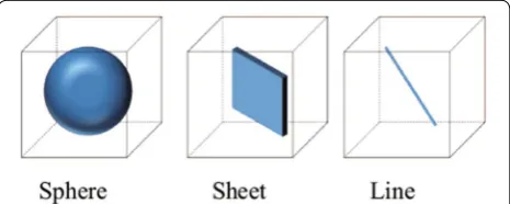
covari-ance matrix of a point cloud in a voxel are obtained. The localization process uses these eigenvalues and eigenvec-tors to extract representative planes and compares the map data with the measured data using a particle filter. In the spatial change detection, according to the following criteria for the eigenvalues, we classify the point distribu-tion in ND voxels into three categories, that is, “Sphere”, “Sheet”, and “Line” (Fig. 3). In addition, if there are no measured points in a voxel, then we refer to the voxel as “Empty”. Thus, one of four labels, “Sphere”, “Sheet”, “Line”, and “Empty”, is assigned to each voxel.

Magnusson et  al. [31] also proposed a loop detection technique using the histogram of three shapes (spherical, planar, and linear), which are classified from point clouds according to the eigenvalues. In our case, we use these

(1)

Sphere _3≈2≈1≫0

(2)

Sheet _3≈2≫1≈0

(3)

Line ₃≫₂≈₁≈0

classifications to evaluate the difference between the map and measured voxels.

If the voxels in the map and measured data are labeled with different categories, then we say that there is a spatial change in this space of the voxel. However, this technique cannot distinguish between similarly shaped objects. Thus, in addition to the technique above, we compare the normal or direction vectors of the sheets and the lines, which are the eigenvectors corresponding to minimum and maximum eigenvalues, respectively. If these vectors are sufficiently matched, then we consider that these voxels to have the same labels and ignore their spatial change. On the other hand, if both voxels have the same labels of “Sheet” or “Line”, but normal or direction vector of the sheet or line is significantly different, we consider there are spatial changes.

where n and v are the normal and direction vectors of the sheets and the lines which are eigenvectors corre-sponding to the smallest and the largest eigenvalues, and Nt and Vt are proper thresholds. nmap and vmap are

cal-culated beforehand from the environmental map (point cloud) measured by a 3D laser scanner, and nmeasured and vmeasured are obtained using the measured map (point cloud) by an on-board range sensors. In the experiments in “Experiments in indoor and outdoor environments” section, we set Nt and Vt as 0.5. Similar idea can be seen in [23], in which “best fitting plane orientation” was used to evaluate the spatial changes.

Overlapping of voxels in map data

The proposed technique inherently involves a quantiza-tion error because we divide the entire space into sev-eral voxel grids and perform NDT for each voxel. Thus, the classification mentioned above is also affected by the quantization error. For example, the boundary between a floor and a wall is classified as “Sheet” if the majority of points in the voxel belong to either a floor or a wall. On the other hand, the boundary is classified as “Sphere” if both planes are evenly included.

In order to suppress the influence of quantization error, the proposed technique uses overlapping ND voxels [9]; that is, adjacent voxels overlap each other so that the centers of the voxels are displaced with half the voxel size, as shown in Fig. 4. As a result, every point in 3D space is involved with eight adjacent voxels since the voxels are overlapped with half the voxel size. In practice, 27 adjacent voxels are considered to increase robustness against measurement and localization

(4) (nmap,nmeasured) <Nt (Sheets)

(5) (vmap,vmeasured) <Vt (Lines)

errors. Thus we compare the target voxel in the meas-ured data with up to 27 adjacent voxels in the map data, and if at least one voxel in 27 voxels in the map data is similar enough to the target voxel in the measured data, that voxel is marked as “no change”. By comparing with 27 adjacent voxels, we can evaluate the degree of coincidence of the map and the measured data robustly with respect to the quantization error. Note that, in the proposed technique, overlapped ND voxels in the map can be calculated beforehand in order to reduce the on-line calculation cost.

Voting of spatial change detection through sequential measurements

The measurement data taken from a range sensor are corrupted by noise, and the measurement noise tends to be detected as spatial change in some cases. However, sensor data can be acquired continuously and noise is added randomly. In order to suppress the influence of measurement noise, voting technology through sequen-tial measurements is adopted. Here, we first extract the voxels that are regarded as spatially changed voxels in each measured datum. Then, we vote on these results for the voxels adjacent to the extracted voxel in a global coor-dinate system with the following weights according to the 3D normal distribution. Finally, if the voted score of the voxel becomes larger than a pre-determined threshold, the voxel is marked as “spatially changed”.

where p is the center of the adjacent voxel in the map data and c is the center of the original voxel in the meas-ured data.

In the experiments in “Experiments in indoor and out-door environments” section, we set the voxel size as 400 mm and σ as 200 mm, and voted for the information of the spatial change to 27 adjacent voxels. We implemented the calculation of 3D NDT and the categorization of ND voxels with C++ using the PCL library (ndt_3d.cpp).

(6)

w(p)=N(c,σ2)

Experiments in indoor and outdoor environments Indoor experiments

We conducted experiments in two indoor environ-ments in order to confirm the performance of the pro-posed technique. The mobile robot system used in the experiments is shown in Fig. 5. This robot is equipped with an omni-directional laser scanner (Velodyne HDL-32e) and an RGB-D camera (Kinect for Xbox One, Microsoft).

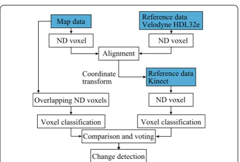
The procedure of localization and spatial change detection is shown in Fig. 6. Firstly, the map data is measured by a precise 3D laser scanner and (over-lapped) ND voxels and their labels (“Sphere”, “Sheet”, “Line”, or “Empty”) are calculated beforehand. For detecting the spatial changes, the reference data meas-ured by Velodyne HDL-32e is transferred to the ND voxels. Then the ND voxels in the map and reference data are compared and the robot position is determined by the NDT-based localization technique in “Fast 3D localization using NDT and a particle filter” section [27]. Obtained coordination transformation informa-tion is applied to the reference data measured by Kinect and ND voxels are calculated. Finally, the overlapped Fig. 4 Overlapping ND voxels

Velodyne HDL-32e

Kinect for Xbox One

Fig. 5 Mobile robot system equipped with an omni-directional laser scanner (Velodyne HDL-32e) and an RGB-D camera (Kinect, Microsoft)

Map data Reference data_{Velodyne HDL32e}

ND voxel ND voxel

Alignment

Coordinate transform

Reference data Kinect

ND voxel

Voxel classification Overlapping ND voxels

Comparison and voting

Change detection

Voxel classification

ND voxels in the map and the ND voxels in the refer-ence data are compared by the proposed technique and the spatial changes are detected.

Spatial change detection in a corridor

Firstly, we conducted an experiment for spatial change detection in a narrow corridor. The environmen-tal map of the corridor was created by scanning from three positions using the high precision laser scan-ner (Faro Focus 3D) beforehand. Figures 7 and 8 show the experimental setup and the positions of five objects placed as spatial changes. The sizes of these objects are

1

�, 40 cm×40 cm×40 cm ; �2, 40 cm×40 cm×120 cm ; 3

�, 40 cm×40 cm×80 cm ; �4, 40 cm×80 cm×40 cm ; and �5, 40 cm×40 cm×80 cm ; respectively. The robot moved straight for 8 [m], turned right at the corner, and moved straight for 7 [m] again. In this experiment, we used the RGB-D camera for the localization instead of the omni-directional laser scanner and captured 75 range images using the RGB-D camera when the robot stopped on the route. These range images were used offline for localization and spatial change detection. The voxel size for localization and the spatial change detection is 40 cm and the number of particles is fix set to be 2000. The pro-cessing time of this experiment is shown in Table 1, and the localization was not processed in real-time since the

RGB-D camera used for the localization takes the huge number of points and the localization takes much time.

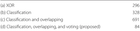
Figure  9a shows the detected regions (red cubes) which are estimated to be spatially changed using XOR calculation of occupied voxels [22]. Figure 9b–d show the detected regions (red, blue, and green cubes) using the classification of point distribution (“Classification of point distributions in ND voxels” section), classification and overlapping of voxels in map data (“Overlapping of voxels in map data” section), classification, overlapping, and voting of spacial changes through sequential meas-urements (“Voting of spatial change detection through sequential measurements” section), respectively. In Fig. 9b–d, detected voxels classified as “Sphere”, “Sheet” and “Line” are illustrated by red, blue, and green cubes, respectively. Table 2 shows the number of voxels detected as spatial changes. As shown Fig. 9d, the regions of spa-tial changes are mostly detected by the proposed tech-nique in “Spatial change detection using ND voxels” section. One region is misdetected as a spatial change. In this region, the measured points by the RGB-D cam-era are classified as “Line” due to the occlusion caused by a single viewpoint. However, this region is classified as “Sheet” in the map created by the high precision laser scanner since no occlusion was occurred in the measure-ment from multiple viewpoints.

In addition, we measured the precise position of the robot when the robot stopped using the laser scanner in order to evaluate the accuracy of localization. The aver-age of the positioning error at 16 positions was 0.171 [m].

Spatial change detection in a hall

Next, we conducted an experiment for spatial change detection in a large hall with dimensions of 40 m×11 m . We placed eight objects having dimensions of �a 10 cm×

10 cm×10 cm ( 1 and 5 ), �b 20 cm× 20 cm×20 cm ( 2 and 6 ), �c 30 cm ×30 cm×30 cm ( 3 and 7 ), and

Fig. 7 Indoor environment (Corridor)

8m

7m

1 2 3

5

4

Fig. 8 Spatial changes (5 boxes)

Table 1 Processing time

Localization 18.04 [s]

Spatial change detection 0.103 [s]

Table 2 Number of voxels detected as spatial changes

(a) XOR 296

(b) Classification 328

d

�40 cm×40 cm×40 cm ( 4 and 8 ) at the positions shown in Fig. 10.

The robot (Fig. 5) then moves along the desired path shown in Fig. 10 automatically and fuses the position information from the particle filter [27] and odometry at 1 Hz. The omni-directional laser scanner is used for the real-time localization. The range data from the RGB-D camera (measured data) are transformed using the esti-mated position information and compared with the envi-ronmental map using the proposed technique. In this experiment, the voxel size for localization and the spatial change detection is 40 cm.

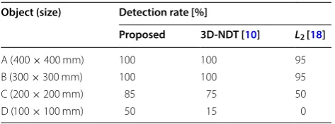
Figure 10 shows the detected spatial changes by the proposed method. Though one region is misdetected as indicated by a white circle, the four kinds of objects that are placed at eight positions later are correctly detected in this experiment. We run the robot from the same ini-tial position to the target position by taking RGB-D data ten times, and obtained the detection rate of the spatial changes as shown in Table 3. Note that we considered the object is detected in case that at least one voxel contain-ing vertexes, edges, or planes of the object is detected as spatially changed.

We also compared the performance of the proposed method with the 3D-NDT based spatial change detection by Andreasson et al. [10], L2 distance function [18], and

simple methods using XOR calculation [22]. The detec-tion rates of the spatial changes for these techniques are shown in Table 3. Figure 11a shows the detected spa-tial changes by the 3D-NDT based method [10]. In this experiment, we used the depth images captured by the RGB-D camera only and the color images were not used. Although the changed regions are mostly detected, some regions are misdetected or undetected.

Figure 11b shows the detected spatial changes by L2

distance function [18]. Figure 11c, d show the detected spatial changes by taking XOR between the map and the measured voxels [22]. Figure 11d uses the overlapped voxels in the map and we judged that the voxel is not spatially changed if at least one voxel among 27 map vox-els adjacent to the measured voxel is occupied. In these experiments using XOR calculation, a number of misde-tected regions are found, which are mainly caused by the positioning error of the mobile robot. On the other hand, the proposed method (Fig. 10) is robust against position error due to voxel classification and voting technique.

voxels distribution

false detection

distribution and overlapping

a

b

c

d

Finally, we show the precision and recall of the detec-tion of voxels which are specially changed for each method in Table 4. We used the overlapped voxels in the map and considered the voxel in the map should be detected as spatially changed if it contains vertexes, edges, or planes of the objects. Table 4 shows that the proposed method, which uses classification of point dis-tribution, overlapping voxels, and voting techniques, gives highest precision (98.50 %) and outperforms other techniques. Figure 12 shows PR and ROC curves for each method using various parameters. In these figures, we can say that the proposed technique outperforms the conventional 3D-NDT [10] and L2 distance based

tech-niques. Note that the recalls are considerably low in all methods. This is because all voxels including at least one vertex, edge, or plane of the object are regarded as the correct voxels to be detected, and therefore, for example,

the voxels on a wall hidden by the object are considered as missing voxels which are not correctly detected.

Table 5 shows the average processing time for one cycle of each step during the experiments (Intel Core i7, 3.40  GHz). The average processing time for spatial change detection by the proposed technique is 20.4  ms including the conversion process of the depth images captured by the RGB-D camera to the ND voxel repre-sentation. On the other hand, the processing time by the 3D-NDT based spatial change detection [10] is 570.0 ms and the proposed technique is 27.9 times faster than the 3D-NDT based technique. The simple method using XOR calculation [22] is slightly faster than the proposed method. Note that, since these processes can be executed independently, we run processes of localization and spa-tial change detection at 1 Hz in the experiments.

Outdoor experiments

We conducted experiments in an outdoor environment. In an outdoor environment, it is very difficult to acquire range data using a RGB-D camera in direct sunlight. Therefore, the omni-directional laser scanner (Velodyne HDL-32e) was used not only for localization but also for spatial change detection. The horizontal resolution of the omni-directional laser scanner is about 1260 points for 360°, and the vertical resolution is 32 lines for 41.3°. Thus, if the space is divided by uniform voxels, the number Initial position

Detected change

Final position 2

3 _{Detected change} 4 _{Detected change}

Misdetected Detected change

Detected change

Misdetected Misdetected 10 m

1 2 3 4

5 6

7 8

Fig. 10 Detected changes. Four kinds of objects placed at eight positions are correctly detected using the proposed method

Table 3 The detection rate for four kinds of objects Object (size) Detection rate [%]

Proposed 3D-NDT [10] L2 [18]

A ( 400×400 _{mm) 100 100 95}

B ( 300×300 _{mm) 100 100 95}

C ( 200×200 _{mm) 85 75 50}

of points measured by the laser scanner at each voxel decreases as it measure long distances. This makes the normal distribution calculation in each voxel very unsta-ble. In addition, the objects in front of the robot should be detected correctly compared to the objects behind. Two techniques are used to overcome these problems; one is to attach the laser scanner to the robot at a slight angle, and the other is to accumulate consecutive scans in each voxel while moving.

Firstly, the omni-directional laser scanner is tilted 15° to increase the resolution of scanning in the front area of the robot as shown in Fig. 13. Figure 14 shows the dif-ference of scan lines with and without tilting the omni-directional laser scanner. If the laser scanner is tilted, the laser beams are densely projected on the floor in front of the robot. In addition, as shown in Fig 15, if a robot moves along a wall, the laser beam is projected diagonally on the wall and the range data is obtained densely as the robot moves. On the other hand, if the laser is not tilted and placed parallel to the floor, the laser beam is pro-jected horizontally on the wall, and no new data can be obtained even if the robot moves.

In addition, in order to increase the number of 3D points in NDT calculation for each voxel, we uses the consecutive scan data assigned to each voxel and the accumulated scan data are converted to ND voxels. In the experiments, two consecutive frames are used for the calculation of ND voxel at once.

In the experiments, we first scan the outdoor environ-ment from three positions using a high-precision laser Misdetected regions

Undetected objects

a 3D-NDT based spatial change detection [10]

Misdetected regions Undetected objects

b L2 distance function [18]

Misdetected regions

c Taking XOR of occupancy voxels [22]

Misdetected regions Undetected objects

d Taking XOR of overlapped occupancy voxels

Fig. 11 Detected changes by a 3D-NDT based spatial change detection [10], bL2 distance function [18], c taking XOR of occupancy voxels [22], and d taking XOR of overlapped occupancy voxels. Misdetected regions and undetected objects are indicated by white circles and crosses

Table 4 Precision and recall [%]

Precision Recall

3D-NDT [10] 61.90 4.79

L2 [18] 81.19 1.11

XOR [22] 17.55 3.95

XOR (overlapped) 69.99 1.71

Classification 22.74 2.47

Classification, overlapping 61.77 26.06 Classification, overlapping, voting

scanner (Faro Focus 3D) and obtained an environmen-tal map. The procedure of the outdoor experiments is shown in Fig. 16. This procedure is almost the same as the procedure in indoor environment shown in Fig. 6, but the on-board sensor for the spatial change detec-tion is changed from Kinect to Velodyne HDL-32e.

We then placed eight objects having dimen-sions of a , 10 cm×10 cm×10 cm at 1 and

0

20

40

60

80

100

0

5

10

15

20

25

30

Proposed

3D-NDT

L₂

Recall

Precisio

n

a

PR Curve

0

5

10

15

20

25

30

0

5 10 15 20 25 30 35 40

FPR

Recall

b

ROC Curve

Proposed

3D-NDT

L₂

Fig. 12 PR and ROC curves in indoor experiment

Table 5 Processing time for each step

Localization Spatial change detection

827.2 [m] 3D-NDT [10] 570.0 [ms]

L2 [18] 17.2 [ms]

XOR [22] 17.9 [ms]

XOR (overlapped) 19.4 [ms]

Proposed 20.4 [ms]

Velodyne HDL-32e tilting 15 degrees

Fig. 13 Mobile robot tilting the omni-directional laser scanner 15°

a Without tilting sparse

b With tilting dense

Fig. 14 Scan lines (black lines) with and without tilting the omni-directional laser scanner

b Laser scanner is not tilted. a Laser scanner is tilted.

Sweep area

Fig. 15 If the laser scanner is tilted, laser beams sweep an object such as a wall along the moving direction densely

Map data Reference data_{Velodyne HDL32e}

ND voxel ND voxel

Alignment

Coordinate transform

ND voxel

Voxel classification Overlapping ND voxels

Comparison and voting

Change detection

Voxel classification Consecutive data Velodyne HDL32e

5

; b , 20 cm×20 cm×20 cm at 2 and 6 ; c ,

30 cm×30 cm×30 cm at 3 and 7 ; and d ,

40 cm×40 cm×40 cm at 4 and 8 as shown in Fig. 17. The robot moved 15 m as shown in Fig. 17 automati-cally while voting spatial changes in 0.5 Hz. Total num-ber of scans by the omni-directional laser scanner is 910 frames. The localization and spatial change detection are processed on-line and in real-time.

Figure 18 shows the detected regions (red cubes) by the proposed procedure while moving the robot. In this experiment, 1 , 2 , 5 cannot be detected because the density of the measured points by the omni-directional laser scanner is not high compared to the RGB-D camera even if the omni-directional laser scanner is tilted.

Table 6 shows the average of the detection ratio by the proposed method, 3D-NDT [10], and L2 [18] after ten

tri-als. In this experiment, the smallest object D cannot be detected by all techniques.

Table 7 shows the precision and recall of the detec-tion of voxels and Fig. 19 shows PR and ROC curves for each method using various parameters. In these figures, we can say that the proposed technique outperforms the conventional 3D-NDT [10] and L2 distance based

techniques. Fig. 17 Spatial changes (8 boxes)

Fig. 18 Detected spatial changes

Table 6 The detection rate for four kinds of objects Object (size) Detection rate [%]

Proposed 3D-NDT [10] L2 [18]

A ( 400×400 mm) 100 100 100

B ( 300×300 _{mm) 100 85 100}

C ( 200×200 _{mm) 50 0 50}

D ( 100×100 _{mm) 5 0 0}

Table 7 Precision and recall [%]

Precision Recall

3D-NDT [10] 59.22 5.63

L2 [18] 79.56 2.76

XOR [22] 9.96 0.91

XOR (overlapped) 42.71 0.34

Classification 13.13 2.54

Classification, overlapping 28.62 28.08 Classification, overlapping, voting

Conclusions

The present paper presented the results of the indoor and outdoor experiments of the fast spatial change detection technique for a mobile robot [8] using an on-board range sensors and a high-precision 3D map created using a 3D laser scanner. This technique first converts point clouds in a map and measured data to grid data (ND voxels) using NDT and classifies the voxels into three categories. The voxels in the map and measured data are then com-pared according to the category and features of the ND voxels. The proposed technique consists of the following three techniques.

1. Classification of the point distribution 2. Overlapping of voxels in map data

3. Voting of spatial change detection through sequential measurements

The contributions of the paper are threefolds:

• We proposed a real-time spatial change detection technique using 3D-NDT and voxel classification. The proposed technique can be integrated with the real-time localization technique [27] using 3D-NDT and a particle filter and reduce the calculation cost. • We implemented the proposed technique using PCL

library and conducted the experiments in indoor and outdoor environments using the RGB-D camera (Microsoft Kinect) and the omni-directional laser scanner (Velodyne HDL-32e).

• Through the experiments in indoor and outdoor environments, we confirmed the proposed localiza-tion and spatial change deteclocaliza-tion techniques can be processed in real-time using on-board sensors and the performance of the proposed techniques outper-forms other cutting-edge techniques.

Future work includes performance evaluation of actual scenes, such as stations or market areas, and

improvement of the performance by using other infor-mation, such as color or laser reflectance. In particular, laser reflectance, which is obtained as a side product of range measurement by a laser scanner, is measured sta-bly independent of the lighting condition, even at night. Therefore, as additional information, evaluating the spa-tial change robustly is very useful.

Acknowledgements

Not applicable.

Authors’ contributions

UK, KM, TI, and TO developed the system and carried out the experiments. AK managed the study. RK constructed the study concept and drafted the manu-script. All members verified the content of their contributions. All authors read and approved the final manuscript.

Funding

Not applicable.

Availability of data and materials

Not applicable.

Competing interests

The authors declare that they have no competing interests.

Author details

1 _{Kyushu University, 744 Motooka, Nishi-ku, Fukuoka-shi, Fukuoka 819-0395,}

Japan. 2 _{Panasonic Inc., 3-1-1 Yagumo-naka-machi, Moriguchi, Osaka 570-8501,}

Japan.

Received: 23 September 2019 Accepted: 5 December 2019

References

1. Hebel M, Arens M, Stilla U (2013) Change detection in urban areas by object-based analysis and on-the-fly comparison of multi-view ALS data. ISPRS J Photogramm Remote Sens 86:52–64

2. Vu TT, Matsuoka M, Yamazaki F (2004) Lidar-based change detection of buildings in dense urban areas. In: 2004 IEEE international geoscience and remote sensing symposium, vol 5, pp 3413–3416

3. Zeibak R, Filin S (2007) Change detection via terrestrial laser scanning. Int Arch Photogramm Remote Sens 36(3):430–435

4. Lague D, Brodu N, Leroux J (2013) Accurate 3D comparison of complex topography with terrestrial laser scanner: application to the Rangitikei canyon (n-z). ISPRS J Photogramm Remote Sens 82:10–26

5. Thomas B, Remco C, Zachary W, William R (2008) Visual analysis and semantic exploration of urban lidar change detection. Comput Graph Forum 27(3):903–910

6. Palma G, Sabbadin M, Corsini M, Cignoni P (2018) Enhanced visualiza-tion of detected 3D geometric differences. Comput Graph Forum 37(1):159–171

7. Li Y, Fan X, Mitra NJ, Chamovitz D, Cohen-Or D, Chen B (2013) Analyz-ing growAnalyz-ing plants from 4D point cloud data. ACM Trans Graph 32(6):157–115710

8. Katsura U, Matsumoto K, Kawamura A, Ishigami T, Okada T, Kurazume R (2019) Spatial change detection using voxel classification by normal distributions transform. In: In proc. IEEE international conference on robotics and automation 2019 (ICRA 2019), pp 2953–2959 9. Biber P, Strasser W (2003) The normal distributions transform: a new

approach to laser scan matching. In: Proceedings 2003 IEEE/RSJ inter-national conference on intelligent robots and systems (IROS 2003) (Cat. No.03CH37453), vol 3, pp 2743–2748

10. Andreasson H, Magnusson M, Lilienthal A (2007) Has something changed here? autonomous difference detection for security patrol robots. In: Proceedings 2007 IEEE/RSJ international conference on intelligent robots and systems, pp 3429–3435

11. Nùüez P, Drews P, Bandera A, Rocha R, Campos M, Dias J (2010) Change detection in 3D environments based on gaussian mixture model and robust structural matching for autonomous robotic applications. In: Proceedings 2010 IEEE/RSJ international conference on intelligent robots and systems, pp 2633–2638

12. Underwood JP, Gillsjo D, Bailey T, Vlaskine V (2013) Explicit 3D change detection using ray-tracing in spherical coordinates. In: 2013 IEEE international conference on robotics and automation, pp 4735–4741 13. Vieira AW, Drews PLJ, Campos MFM (2014) Spatial density patterns for

efficient change detection in 3D environment for autonomous surveil-lance robots. IEEE Trans Autom Sci Eng 11(3):766–774

14. Fehr M, Furrer F, Dryanovski I, Sturm J, Gilitschenski I, Siegwart R, Cadena C (2017) Tsdf-based change detection for consistent long-term dense reconstruction and dynamic object discovery. In: Proceedings 2017 IEEE international conference on robotics and automation, pp 5237–5244

15. Luft L, Schaefer A, Schubert T, Burgard W (2018) Detecting changes in the environment based on full posterior distributions over real-valued grid maps. IEEE Robotics Autom Lett 3(2):1299–1305

16. Palazzolo E, Stachniss C (2018) Fast image-based geometric change detection given a 3d model. In: 2018 IEEE international conference on robotics and automation (ICRA), IEEE, New York, pp 6308–6315 17. Magnusson M, Duckett T (2005) A comparison of 3D registration

algo-rithms for autonomous underground mining vehicles. In: The European conference on mobile robotics (ECMR 2005), pp 86–91

18. Saarinen JP, Andreasson H, Stoyanov T, Lilienthal AJ (2013) 3D normal distributions transform occupancy maps: an efficient representation for mapping in dynamic environments. Int J Robotics Res 32(14):1627–1644 19. Gianpaolo P, Paolo C, Tamy B, Roberto S (2016) Detection of geometric

temporal changes in point clouds. Comput Graph Forum 35(6):33–45

20. Besl PJ, McKay ND (1992) A method for registration of 3-D shapes. IEEE Trans Pattern Anal Mach Intell 14(2):239–256

21. Murakami H, Nakagawa K, Hasegawa H, Shibata T, Iwanami E (1999) Change detection of buildings using an airborne laser scanner. ISPRS J Photogramm Remote Sens 54(2):148–152

22. Spatial change detection on unorganized point cloud data. http://point cloud s.org/docum entat ion/tutor ials/octre e_chang e.php. Accessed 12 Dec 2019

23. Girardeau-Montaut D, Roux M, Marc R, Thibault G (2005) Change detec-tion on points cloud data acquired with a ground laser scanner. Int Arch Photogramm Remote Sens Spatial Inf Sci 36(PART 3):30–35

24. Pollard T, Mundy JL (2007) Change detection in a 3-d world. In: Proceed-ings 2007 IEEE conference on computer vision and pattern recognition, pp 1–6

25. Ulusoy AO, Mundy JL (2014) Image-based 4-D reconstruction using 3-D change detection. In: Fleet D, Pajdla T, Schiele B, Tuytelaars T (eds) Proceedings European conference on computer vision 2014. Springer, Cham, pp 31–45

26. Scona R, Jaimez M, Petillot YR, Fallon M, Cremers D (2018) StaticFusion: background reconstruction for dense RGB-D slam in dynamic environ-ments. In: 2018 IEEE international conference on robotics and automa-tion (ICRA), IEEE, New York, pp 1–9

27. Oishi S, Jeong Y, Kurazume R, Iwashita Y, Hasegawa T (2013) ND voxel localization using large-scale 3D environmental map and RGB-D camera. In: Proceedings 2013 IEEE international conference on robotics and biomimetics (ROBIO), pp 538–545

28. Nuchter A, Surmann H, Lingemann K, Hertzberg J, Thrun S (2004) 6D slam with an application in autonomous mine mapping. In: Proceedings IEEE international conference on robotics and automation 2004, vol 2, pp 1998–2003

29. Nüchter A, Lingemann K, Hertzberg J, Surmann H (2007) 6D slam—3d mapping outdoor environments: research articles. J Field Robotics 24(8–9):699–722

30. Olson CF, Matthies LH (1998) Maximum likelihood rover localization by matching range maps. In: Proceedings 1998 IEEE international confer-ence on robotics and automation (Cat. No.98CH36146), vol 1, pp 272–277 31. Magnusson M, Andreasson H, Nuchter A, Lilienthal AJ (2009)

Appear-ance-based loop detection from 3D laser data using the normal distribu-tions transform. In: Proceedings 2009 IEEE international conference on robotics and automation, pp 23–28

Publisher’s Note