www.atmos-meas-tech.net/9/347/2016/ doi:10.5194/amt-9-347-2016
© Author(s) 2016. CC Attribution 3.0 License.
Mobile sensor network noise reduction and recalibration
using a Bayesian network
Y. Xiang, Y. Tang, and W. Zhu
College of Information Engineering, Zhejiang University of Technology, Hangzhou, China Correspondence to: Y. Xiang ([email protected])
Received: 13 May 2015 – Published in Atmos. Meas. Tech. Discuss.: 31 August 2015 Revised: 17 January 2016 – Accepted: 23 January 2016 – Published: 4 February 2016
Abstract. People are becoming increasingly interested in mobile air quality sensor network applications. By eliminat-ing the inaccuracies caused by spatial and temporal hetero-geneity of pollutant distributions, this method shows great potential for atmospheric research. However, systems based on low-cost air quality sensors often suffer from sensor noise and drift. For the sensing systems to operate stably and reli-ably in real-world applications, those problems must be ad-dressed. In this work, we exploit the correlation of different types of sensors caused by cross sensitivity to help identify and correct the outlier readings. By employing a Bayesian network based system, we are able to recover the erroneous readings and recalibrate the drifted sensors simultaneously. Our method improves upon the state-of-art Bayesian belief network techniques by incorporating the virtual evidence and adjusting the sensor calibration functions recursively.
Specifically, we have (1) designed a system based on the Bayesian belief network to detect and recover the abnormal readings, (2) developed methods to update the sensor calibra-tion funccalibra-tions infield without requirement of ground truth, and (3) extended the Bayesian network with virtual evidence for infield sensor recalibration. To validate our technique, we have tested our technique with metal oxide sensors measur-ing NO2, CO, and O3in a real-world deployment. Compared
with the existing Bayesian belief network techniques, results based on our experiment setup demonstrate that our system can reduce error by 34.1 % and recover 4 times more data on average.
1 Introduction
compounds or acids, aging, or condensate on the sensor sur-face (Haugen et al., 2000; Arshak et al., 2004). Sensor drift changes the sensor function, which can cause significant de-viation from the ground truth without proper error compen-sation. For example, in our own deployment, we find that the sensor drift can increase the average sensor error by orders of magnitude within several months. Drifted sensors must be recalibrated before they can be trusted and used again.
The metal oxide sensors, utilizing either the oxidation or reduction reactions with pollutant gases, can respond to and quantify the air pollutants with reasonable sensitivity and ac-curacy (Tans and Thoning, 2008). However, many pollutants share the same reaction property. For example, both CO and NO2can cause oxidation reactions with the surface material.
Thus, the sensors usually respond to a wide range of pollu-tants other than the targeting gas. This property is called cross sensitivity (Zampolli et al., 2004). Because of cross sensi-tivity, the readings of different types of sensors are usually correlated. This property can be used to identify the compo-sitions of pollutants in the environment (Di Lecce and Cal-abrese, 2011).
We leverage the correlations of different metal oxide sen-sors to help identify and recover the abnormal readings. In many recent mobile sensing network designs, researchers have built sensing devices equipped with multiple types of sensors to detect various pollutants co-existing in the envi-ronment (Jiang et al., 2011; Willett et al., 2010). For such applications, it is possible to exploit the correlation of read-ings and recover noisy readread-ings using Bayesian belief works (Janakiram et al., 2006). The basic Bayesian net-work approach net-works well for the outliers caused by random noises but fails when sensors drift, which is common in real-world applications.
In this work, we aim to design a system that can efficiently detect and recover the noisy readings, recalibrate drifted sen-sors, and identify the gas compositions in the air simultane-ously. This work makes the following contributions:
1. we have designed and implemented a Bayesian belief network based system to detect and recover outliers; and 2. we incorporate and address the sensor function calibra-tion problem within the Bayesian network framework. By analyzing the collected data, we have observed signif-icant drift within a short period of time, e.g., a couple of months for most of the sensors. To validate our hypothesis and techniques, we have performed a field deployment. The deployment lasts about 3 months. During the deployment, we have mainly monitored and analyzed the following air qual-ity related gases: NO2, CO, and O3. The deployment results
have confirmed our models about the sensor drift and the ef-fectiveness of our techniques.
The rest of this paper is organized as follows. Sec-tion 3 discusses existing related work. SecSec-tion 4 provides an overview of the system. Section 5 describes the Bayesian
belief network approach and how to use it to detect and re-cover outliers. Section 6 discusses the limitations of exist-ing Bayesian network approaches and presents our solution. Section 7 describes our real-world deployment and the eval-uation results of different techniques.
2 Motivation example
This work is motivated by an atmosphere research project. Researchers have built several mobile atmosphere monitor-ing devices and deployed them in the field to monitor the atmosphere around the users. The devices can measure mul-tiple pollutant gases using metal oxide sensors. Those sen-sors are precalibrated in the lab and are hence accurate before deployment. However, after a couple of months, it is discov-ered that the sensitivities of the sensors have shifted signif-icantly, which can lead to erroneous scientific conclusions, false alarms, incorrect decisions, etc. Therefore, it is benefi-cial and important to develop a technique that can utilize the relationship between different types of sensors to reduce the sensor noise and recalibrate the sensors during deployment.
3 Related work
The related work can be placed in three categories: co-located sensor calibration, sensor abnormality detection, and Bayesian network based approaches.
3.1 Co-located sensor calibration
Xiang et al. (2012, 2013) developed a model to estimate sen-sor drift and designed a compensation technique to minimize the sensor drift assuming no access to ground truth readings. Bychkovskiy et al. (2003) have proposed a two-phase post-deployment sensor drift compensation technique in which co-located sensors are calibrated in pairs using linear func-tions. Miluzzo et al. (2008) have proposed CaliBree, an auto-calibration algorithm for mobile sensor networks, in which mobile sensor nodes opportunistically interact with accurate stationary sensors and hence enable calibration to reduce sor drift. Those techniques require that the co-located sen-sors are of the same type and thus should have the same response from the physical environment. In contrast to the previous work, our technique can work on mobile sensing devices containing various types of metal oxide sensors. 3.2 Sensor abnormality detection
classify and identify the local outliers. Unlike our technique, their method cannot estimate the actual ground truth readings and recover outliers. Papadimitriou et al. (2003) have devel-oped a technique that uses multi-granularity deviation factor to dynamically detect the outlier readings based on the cor-relations of local nodes. Their technique cannot address the sensor drift problem, however, when one or more sensors’ readings are shifted persistently. Kumar et al. (2013) pro-posed a technique that performs a two-stage drift correction. First, they use a Kriging based approach to provide estimated ground truth readings. Then a Kalman filter based technique is used to compensate for sensor drift. However, Kriging re-quires certain spatial density in sensor nodes deployment. Moreover, a Kalman filter based approach relies on the as-sumption of a state-space underlying model and knowledge of the model parameters, which is unrealistic in real-world applications when the environment of the deployment field is often unknown and very dynamic.
3.3 Bayesian network based approaches
Elnahrawy and Nath (2003) have used a naive Bayesian net-work to identify local outliers and detect faulty sensors. This technique uses a trained Bayesian classifier for probabilistic inference. Each node locally computes the probabilities of each of its incoming readings and determines the readings as outliers when their probabilities are not the highest among all the possible outcomes. Their approach can only work for the homogeneous sensors. Janakiram et al. (2006) have pro-posed a technique to detect sensor outliers based on Bayesian belief network. They leverage the conditional correlation of the readings from different types of sensors. However, their approach does not take into consideration sensor drift and sensor function recalibration, which are considered and ad-dressed by our method.
4 System flow
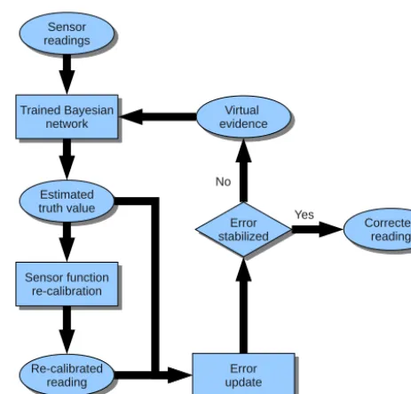
Figure 1 shows the overview of our system. It describes the composition of the system. In the real-world applications, the gathered atmosphere data, e.g., O3, are processed by the
sys-tem. The system can reduce the sensing error caused by drift as well as other atmospheric parameters and recalibrate the sensor function. The output of the system is the O3data with
significantly improved accuracy and a more sensitive sensor function.
The input sensor readings are first processed using a Bayesian belief network, which is trained using normal data from the infield deployment. The Bayesian network can gen-erate the estimated ground truth values based on the condi-tional probability tables and readings from all the correlated sensors. The estimated ground truth readings are then used to recalibrate the sensors, i.e., generate the new sensor functions which can translate the input sensor analog readings into ac-tual pollutant concentrations. The new sensor functions are
Trained Bayesian network
Trained Bayesian network
Estimated truth value
Estimated truth value
Sensor readings
Sensor readings
Sensor function re-calibration
Sensor function re-calibration
Re-calibrated reading
Re-calibrated
reading updateupdateErrorError
Virtual evidence
Virtual evidence
Error stabilized
Error
stabilized CorrectedCorrectedreadingreading Yes
No
Figure 1. System flow.
used to generate the sensor readings, which are used to de-rive the estimated error. The newly updated estimated error is compared with the previous estimations. If the variation is within a certain threshold, we consider the system stabi-lized and the current results to be the best estimation and final output. If the system is not stabilized yet, the virtual ev-idence, which describes the error distributions of the input data, is updated using the new estimated concentration and subsequently used by the Bayesian network to generate the estimated ground truth readings for the next round of opti-mization. The loop continues after a certain number of runs or until the system converges.
5 Basic Bayesian belief network
In this section, we first introduce the basic Bayesian belief network. Then we discuss how to implement it in real-world applications.
5.1 Bayesian network introduction
Bayesian networks are widely used to detect and recover ab-normal data points for sensor networks. The Bayesian net-work is built based on Bayes’ theorem and capable of ex-ploiting the interdependent or causal relationships of corre-lated sensors readings. The types of the sensors involved can be different, which makes it appropriate for our application. A Bayesian network is a directed graph consisting of nodes and arcs (Kay, 1998).
T.
T.
NO2
NO2 COCO
T1
T2 0.5
0.5
T.
T1
T2 0.3
0.7 NO2
T.
N1
N2 0.1
0.6 CO NO2 N1 N2
0.4
0.6
T1
T1 T.
N1 N2 T2 T2
0.5 0.2 C1 C2
0.9
0.4 0.5 0.8
Figure 2. An example of a Bayesian belief network.
Each sensor’s readings can be discretized intoNvalues, with each discrete value denoted asTn, Cn, and NOn, respectively. Without loss of generality, we assume two distinct discrete values for each sensor type. All the metal oxide sensors are correlated because of cross sensitivity. The readings of metal oxide sensors are strongly affected by the temperature. We found no significant impact from relative humidity.
As shown in the figure, the Bayesian network describing this sensor network contains three nodes, with each repre-senting one type of sensor. There are two arcs connecting the temperature sensor with the metal oxide sensors and one arc connecting the two metal oxide sensors. To calculate the probability inference of each variable given the input of other variables as evidence, each node is associated with a table, which is called conditional probability table (CPT). CPT de-scribes the conditional dependence between any node with its parents. For the root node with no parents, CPT describes the distribution of the variable itself. CPT can be derived by training the network using historic data.
5.2 Bayesian network for real-world applications
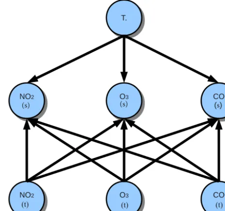
Without loss of generality, we assume that there are four types of equipped sensors: temperature, NO2, CO, and ozone
(O3). Their readings are all correlated. The Bayesian network
graph for this application is shown in Fig. 3. In the graph, there are two types of nodes. The first type, which contains T, CO(s), NO2(s), and O3(s), represents the readings of the
sensors. The second type, which contains CO(t), NO2(t), and
T.
T.
NO
NO2 CO
(s) CO
O
O3
(s)
NO
NO2 OO3 COCO
(s)
(t) (t) (t)
Figure 3. The basic Bayesian network structure for our application.
(Symbols with (s) are referred to the sensor readings; symbols with (t) are referred to the ground truth concentrations.)
O3(t), represents the actual concentration (ground truth) of
the corresponding pollutants in the environment.
In the figure, there are arrows connecting the temperature sensor to all the three types of metal oxide sensors since the temperature influences the measurement results of all the three metal oxide sensors. The metal oxide sensors are as-sumed to be independent from each other, and the same is true for the ground truth concentration nodes. However, be-cause of cross sensitivity, each ground truth reading can have significant impact on the readings of three metal oxide sen-sors simultaneously. Thus, there are three arcs connecting the ground truth concentrations to all the three sensors. When the ground truth is not available, the probability inference of the three ground truth nodes can be calculated using the input of the four actual sensors. The value with the highest probabil-ity is considered as the estimated ground truth, as shown in the following equation.
G(i)= max
n∈N (i)(Pn(i)), (1) whereG is the ground truth reading for sensori,N is the number of possible values after discretization, andP is the probability.
6 Bayesian network with sensor recalibration
the drift problem and the sensor recalibration technique to improve the performance of the Bayesian network. Finally, we present the combined recursive system and describe the details and algorithm to implement it.
6.1 Problems for basic Bayesian network
Bayesian network can clean the corrupted data and detect ab-normal readings by leveraging the interdependency of corre-lated sensors. For the random noises, it is quite efficient and sufficient. However, in our applications, sensors frequently drift. It has been shown, both in existing literature (Xiang et al., 2012; Romain and Nicolas, 2010) and by our own measurement data presented in Sect. 7.1.3, that sensor drift is a very common and severe problem in real-world applica-tions for those metal oxide sensors. Sensor readings become useless with the bias observed in our deployment. Thus, the problem of sensor drift and the error caused by drift must be addressed.
The basic Bayesian network is based on the assumption of unbiased measurements. Thus, it is unable to generate rea-sonable results when multiple sensors drift simultaneously. Note that it is quite common to have more than one drifted sensors in the system simultaneously, as shown by our de-ployment results in Sect. 7.1. Thus, the system described in Fig. 3 is inadequate to address the real-world problems. To apply the Bayesian network in such circumstances, we need to (1) incorporate a ranking mechanism that can quantify the sensor uncertainties into the Bayesian network and (2) design a drift compensation scheme to recalibrate the sensor func-tion and recover the corrupted data simultaneously within the Bayesian network framework.
6.2 Error distribution and uncertain evidence
As the sensor drifts, its sensing sensitivity deteriorates and the uncertainty of its readings increases. A Bayesian net-work treats all its input equally, which is problematic consid-ering sensor drifts. For example, if a CO sensor is recently calibrated while an O3 sensor has not been calibrated for a
long time, we should clearly give the CO sensor more confi-dences. In other words, within a Bayesian network frame-work, we must have an evaluation mechanism which can rank and quantify the trustworthiness of each particular sen-sor.
To address this problem, we use error distributions to rep-resent the sensitivity and trustworthiness of the sensors. An example of error distributions is shown in Table 1. In the example, we assume that the sensor has reported an envi-ronment concentration of 1.5 ppm. The actual ground truth ranges from 0 to 3 ppm and is divided into three discrete cat-egories. We assume that in the environment the probability for the ground truth to be in any of these three categories is equal. As shown in Table 1, if the sensor is accurate, then the probability that the actual ground truth is within the range of
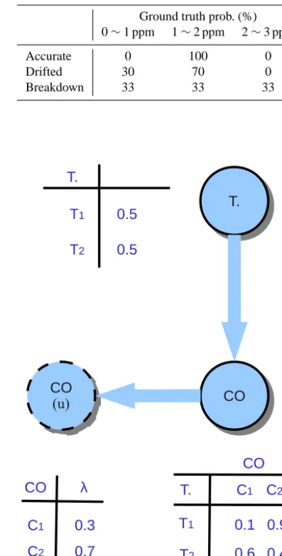
Table 1. An example error distribution with reported reading of
1.5 ppm.
Ground truth prob. (%) 0∼1 ppm 1∼2 ppm 2∼3 ppm Accurate 0 100 0 Drifted 30 70 0 Breakdown 33 33 33
T. T.
CO CO
CO CO T1
T2
0.5
0.5
CO
C1 C2
0.3 0.7
T.
0.1
0.6 CO
T1 T.
T2
C1 C2
0.9
0.4 λ
(u)
Figure 4. An example of virtual node. (Symbol with (u) is referred to the virtual node.)
1 to 2 ppm given a reported reading of 1.5 ppm is 100 %. If the sensor is drifted, the sensor becomes less accurate and the possible value of the ground truth spreads wider. If the sen-sor has a breakdown, it loses most of its sensitivity and the ground truth is no longer correlated to the sensor readings.
Table 2. The statistics of the original and drifted sensor readings.
Errors
Undrifted Drifted CO NO2 O3 CO NO2 O3 (ppm) (ppb) (ppm) (ppm) (ppb) (ppm) Average 0.31 16.13 0.04 10.72 112.45 0.20 Maximum 8.92 76.11 0.32 21.94 171.4 1.85 Standard deviation 0.52 11.19 0.07 0.93 12.50 0.28 Correlation 93 %
6.3 Bayesian network with virtual evidence
For the basic Bayesian network, the inputs can only be deter-mined values. To incorporate the virtual evidence, some con-straints must be honored, which is called Jeffrey’s rule (Jef-frey, 1990). The concept of Jeffrey’s rule is described as fol-lows.
Suppose the universe of all the events is denoted asU. We have a set of mutually exclusive events γ1, . . ., γn, which is a subset ofU, andP is the probability distribution of those events. After applying the virtual evidence, the beliefs for eventsγ1, . . ., γn change and the updated distribution is de-noted asP0.P0should satisfy the following equation. P (α|γi)=P0(α|γi),∀i=1, . . ., n, (2) whereα is any event in the universe. In other words, after the virtual evidence is accepted, the posterior probability of αcan be changed, but the conditional probability forα∈U regarding to the eventsγ1, . . ., γnmust remain the same.
To treat the virtual evidence as determined value while honoring the Jeffrey’s rule, the Bayesian network should be modified by adding a virtual node to the drifted sensor nodes (Chan and Darwiche, 2005). Figure 4 shows an ex-ample Bayesian network with virtual nodes. In the figure, the pollutant followed by V represent a virtual node in the Bayesian network. The number in Table 2 is the conditional probability. λ represents the probability distribution of the input evidence. There are two sensor nodes: temperature and CO. The temperature sensor is assumed to be accurate and with little drift, while the CO sensor can drift. The CO sen-sor node is associated with a virtual node, denoted as CO(u). The virtual node also has its own conditional probability ta-ble. The CPT of the virtual node should be calculated us-ing the error distribution of the actual sensor node so that the beliefs of the whole Bayesian network comply with Jef-frey’s rule. The detailed methods and equations to calculate its probability table can be found in existing literature (Peng et al., 2010; Chan and Darwiche, 2005). Note that the virtual node is only dependent on the corresponding sensor node and independent of all the other nodes in the network.
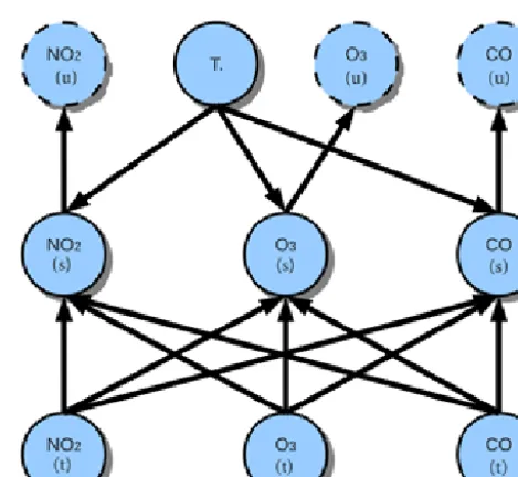
Figure 5 shows the Bayesian network structure of our ap-plication after incorporating the virtual evidence. Since the temperature sensor and the hypothetical ground truth
con-Figure 5. The Bayesian network with virtual nodes. (Symbol
defi-nition in Sect. 5.2.)
centration sensors are assumed to be accurate, they are not associated with any virtual nodes. Each metal oxide sensor, which is prone to drift, is associated with a virtual node. The contents in the CPT of the virtual nodes can be calculated us-ing the error distributions of the actual nodes, which can be derived with the information of the (estimated) ground truth readings and the sensor readings.
6.4 Sensor function recalibration
The transformation function to translate the analog input sig-nal into pollutant concentration is called a sensor calibration function, or sensor function. The abnormal readings caused by environmental noises do not reflect a change of the sen-sor function. However, when sensen-sors are drifted, the sensen-sor functions change, which can cause a systematic increase of abnormal readings.
In this work, we apply a piece-wise linear function as the sensor function, which is shown in the following equation.
whereC is the pollutant concentration,pi are the fitting pa-rameters, V is the voltage, and T is the temperature. The temperature information is reported by the on-board sensors. Note that for our experimented sensors, the impact of humid-ity is much less significant than temperature. Thus, we do not include humidity in our setup. If parameters in other applica-tions, such as humidity and pressure, do have significant im-pact, they can be easily incorporated to our Bayesian frame-work. The parameters in the equation are derived using lin-ear regression with the training data. Since accurate sensors providing ground truth readings are usually not available, we use the estimated ground truth concentration returned by the Bayesian network instead. Note that as the sensitivity of the sensors reduces, the performance of this recalibration scheme deteriorates. When a sensor breaks down and loses most of its sensitivity, the sensor can no longer be recalibrated.
7 Experimental results
In this section, we first describe a real-world co-location de-ployment of nine mobile sensor nodes and the analysis re-sults for the deployment data. We then evaluate our system using the real-world data.
7.1 Mobile sensor network deployment and analysis 7.1.1 The mobile sensing device
To investigate the effect of sensor drift in real-world applica-tions and collect data to evaluate our data cleaning technique, we deployed a sensor network in Denver, Colorado. Dur-ing the experiment, we deployed nine M-Pods (Jiang et al., 2011), which are shown in Fig. 6. The M-Pod is a custom-built mobile sensing device supporting embedded sensing, computation, and wireless communication. It supports detec-tion of various air pollutants, including NO2, CO, CO2, O3,
and volatile organic compounds. It can also measure temper-ature, humidity, and light. The latest revision of the M-Pod is compact (5×6.5 cm) and energy efficient, with a battery life of greater than 16 h. The whole device, including a Li-ion battery with a capacity of 6000 mA-h, is enclosed by a low-cost off-the-shelf case that can be carried using an armband or attached to a backpack. A[3.3] V DC fan is used to control airflow. A rectangular filter is installed around sensor to in-crease sensing accuracy and prolong sensor life. Most of the power-hungry on-board sensors are power gated and can be controlled by commands from smartphones. Data are tempo-rally stored in a 1 megabyte non-volatile EEPROM. The to-tal cost of the on-board components and sensors is less than USD 150 and can be reduced further when produced in large quantities.
To receive, store, and present the data gathered by our M-Pod device, we have developed on-board firmware, smart-phone applications, data servers, and Web interfaces. The firmware defines protocols of sensing, storing, and sending
the environmental data. The smartphone application commu-nicates with the M-Pod via its Bluetooth interface. It can is-sue commands to and receive data from the M-pod. The data are transmitted to the online data server and stored in the databases. A Web based user interface allows users to access and analyze air quality data.
7.1.2 The real-world deployment
The nine M-Pods were used continuously from March to May 2013. The sensors were not changed throughout this pe-riod. For the majority of the time, the M-Pods were worn by users as part of an exposure assessment study. During three multi-day calibration periods in March, April, and May, the M-Pods were placed at a reference air quality monitoring site. The M-Pods were powered continuously on the roof of the monitoring building, in a ventilated enclosure near the air inlets for the reference monitors. The reference site, as shown in Fig. 6, monitors CO, NO2, and O3. It is located in
down-town Denver, Colorado, and operated by the Colorado De-partment of Public Health and Environment (CDPHE). The highly accurate and regularly maintained air pollutant moni-toring equipment in the station is used to provide the ground truth readings.
By co-locating the M-Pods with the reference monitors, we are able to derive both the sensor analog readings and ground truth, which can be used to determine the sensor cal-ibration functions. The forms of the sensor calcal-ibration func-tions vary depending on sensor type. In this work, we use a piece-wise linear function. It is quite accurate according to lab and field measurements and requires much fewer re-sources to compute compared to other, more complicated, forms of sensor functions. The calibrations are performed us-ing the field data. Thus, it does not require specialized equip-ment and can cover a wider range of environequip-mental parame-ter space than lab calibrations. Before the fitting of the sen-sor function, data filtering was performed to remove noise from the sensor readings. Minute medians were first calcu-lated from the 6 s raw data. Then, we applied a filter based on difference in consecutive differences in the medians. There were two thresholds for the filter: an absolute threshold that was deemed unrealistic based on lab experiments and 2 times the standard deviation of the differences. By performing cal-ibrations periodically with the same sets of sensors, we were able to assess the change in baseline readings and sensitivity over time. The calibration functions derived by fitting to the data of the first calibration period, which is considered as the undrifted baseline, are applied to the entire data set.
7.1.3 Data analysis
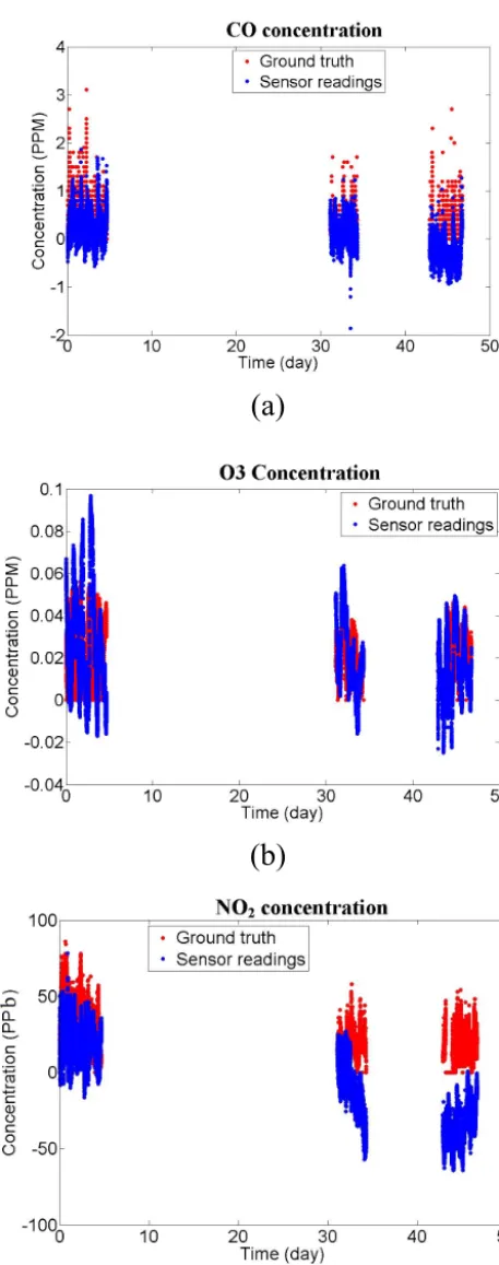
We examine and compare the readings of the CO, NO2, and
O3 sensors. An example of the measured data and the
(a) (b)
Figure 6. (a) The Denver air quality monitoring station; (b) the M-Pod sensing platform.
in the unit of days, while the Y axis shows the concentra-tion of the pollutant in parts per million. Two sets of data are presented: ground truth data and M-pod measured data. The total duration of the deployment is about 2 months. In the fig-ure, there are three separate time periods, with each lasting for about 1 week. During that time period, the M-Pods are located in the station and calibrating. For the rest of the time, the M-Pods are carried by individual users and the ground truth readings of their exposed environments are unknown. Thus, the readings from those time periods are not included. The resultant data show that the drift rates for different types of sensors vary. For the example in the figure, the NO2
sensor experiences large drift. After 2 months, its drift er-ror is increased more than 3 times. The CO sensor also suf-fers significant drift, though less compared to the NO2sensor
with about 50 % increase of error. However, for the O3
sen-sor, no significant drift is observed. The example shows that significant drift can occur within just a couple of months, ren-dering the corresponding sensor almost useless if not care-fully recalibrated. It demonstrated that drift is a real and se-vere challenge for those cheap sensors to be useful in real-world applications. Moreover, since the exposed environ-ment and the properties of the sensors vary, different sensors usually exhibit different drift rates, making it impossible to recalibrate the sensors using a predetermined model.
Among the nine M-Pods deployed, we chose six of them during our analysis and evaluations. For the rest three, one of them did not return enough data due to transmission problem, and two of them have sensors completely dead within the 2-month deployment period. Table 2 shows the statistics of the sensing errors from the remaining six M-Pods. The error in the table are defined as the absolute variation between the sensor reading and the ground truth. We compare the drifted and undrifted data. The undrifted data are taken from the first time period as shown in Fig. 7. The drifted data are taken from the third time period. The first three rows show the av-erage, maximum, and standard deviation of the error
distri-butions. Significant drift can be observed for all the types of sensors. It should be noted that for some pollutants, such as NO2 and CO, their mean values change more significantly
than the standard deviation, which implies a close to linear shift. For each pair of sensors, e.g., NO2and O3, their
corre-lation coefficient is calculated. Among all the possible pairs, 93 % of them show a strong correlation, indicating that the Bayesian network might be an appropriate solution.
In conclusion, our deployment data show that sensor drift and consequently the noise problem are very realistic and im-portant for the metal oxide sensors. If not properly addressed, most of those sensors will be useless within just a couple of months. The drift rates are dependent on the environment and sensor properties and, hence, vary for different sensors. Thus, it is not feasible to use predetermined correction meth-ods; sensor calibration problem must be addressed using the field data. Moreover, different types of sensors show strong correlations, permitting noise reduction and sensor calibra-tion.
7.2 Data recovery and sensor calibration results 7.2.1 Experiment setup
(a)
(b)
(c)
Figure 7. (a) Drift measurement of CO; (b) drift measurement of
O3; (c) drift measurement of NO2.
The CPT of the Bayesian network is derived from train-ing. The training set is generated using the co-location data from the undrifted (the first) time period. This approach is more appropriate since it requires much less effort to cover a reasonable number of states than lab environment and can provide us a more realistic prior distributions for tempera-ture. The training data set is filtered so that it contains only normal data. After the Bayesian network is trained, the con-tents in the CPT remain unchanged until the sensor is close to a reference station and have access to the ground truth read-ings again. For the parameter states that are not encountered during the training phase, we replace their contents with the encountered state of the closest distance, calculated using the Euclidean distance between those two states.
To evaluate our outlier recovery and sensor recalibration technique, we compare the following three approaches.
1. Uncompensated: this approach interprets the reported analog data using the predetermined sensor function from lab measurement and without any compensation scheme.
2. Bayesian network: this approach implements a Bayesian belief network based technique proposed by Janakiram et al. (2006). It is the most relevant and closely related work to the best of our knowledge.
3. Bayesian network with virtual evidence: this is our pro-posed technique. It improved upon the Bayesian net-work approach by incorporating the virtual evidence and sensor recalibration.
We evaluate all the three approaches using the same set of testing data derived from our real-world deployment. 7.2.2 Drifted sensor recovery evaluation
Figure 8. The data recovery results of various techniques for the
drifted data.
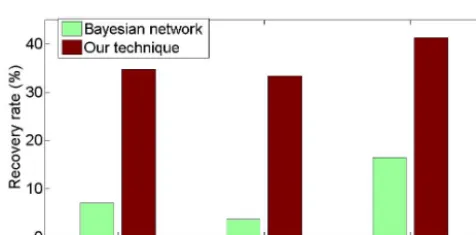
Figure 9. The percentage of successfully cleaned data.
about 2.13 % error on average. Moreover, compared with the Bayesian network approach, which is the closest exist-ing technique, our technique is capable of reducexist-ing errors by 32.0, 34.7, and 35.5 % for CO, NO2, and O3, respectively. In
our setup, the experiment results show that our technique can reduce error by 34 % on average.
After the estimated ground truth values are derived, we consider it the ground truth concentration. However, since the ground truth concentration estimation is imperfect, the classification of sensor readings according to this estimate ground truth concentrations can be wrong. Hereby we de-fine data recovery rate as the percentage of corrected label data points after the data recovery scheme. Figure 9 shows the comparison results of various techniques in terms of data recovery rate. The rate is obtained by comparing the esti-mated readings against the ground truth. For our technique, the data recovery rates are 34.7, 33.3, and 41.3 % for CO, NO2, and O3, respectively. Compared with the Bayesian
net-work approach, our technique successfully recovers 4 times more data.
8 Conclusions
In this work, we have presented a Bayesian belief network based system to detect and recover outliers in the presence of sensor drift. This work is to address the data noise and sensor drift problems in atmospheric research by exploring the correlation of different types of sensors. In our analysis of real-world data, low-cost air quality sensors usually in-cur significant drift within a few months. Thus, to ensure the accuracy of the atmosphere researches utilizing those sen-sors, we developed a data treatment technique that can sig-nificantly reduce the sensor noise and recalibrate the drifted sensor online.
Our technique can significantly improve sensor accuracy given the cross-correlation of sensors for different gasses. Thus, it is most suitable for applications involving sensor clusters, such as mobile environmental sensing, health moni-toring, and hazard gas alert. However, for the more traditional monitoring methods, which rely upon accurate and singular sensors, the applications of our technique are more limited.
Nonetheless, there are many areas for improvements in the future research. This technique, along with other Bayesian network based techniques, requires extensive training prior deployment. However, with limited training data, offline training can introduce inaccuracies with untrained events. Thus, it is important to develop online Bayesian network based training techniques alongside the calibration tech-nique. Moreover, the response time of different sensors may differ with each other. Thus, the technique should be adapted to address sensors with variable response time. Bayesian network based techniques can also be used for sensor network malfunctioning analysis and diagnosis, which is another important application area.
Edited by: P. Stammes
References
Arshak, K., Moore, E., Lyons, G. M., Harris, J., and Clifford, S.: A review of gas sensors employed in electronic nose applications, Sensor Rev., 24, 181–198, 2004.
Bayes toolbox: Bayes Net Toolbox for Matlab, https://code.google. com/p/bnt/, last access date: 19 October 2007.
Bettencourt, L. M., Hagberg, A., and Larkey, L.: Separating the Wheat from the Chaff: Practical Anomaly Detection Schemes in Ecological Applications of Distributed Sensor Networks, Lect. Notes Comput. Sc., 4549, 223–239, 2007.
Bychkovskiy, V., Megerian, S., Estrin, D., and Potkonjak, M.: A collaborative approach to in-place sensor calibration, Lect. Notes Comput. Sc., 2634, 301–316, 2003.
Chan, H. and Darwiche, A.: On the revision of probabilistic beliefs using uncertain evidence, Artif. Intell., 163, 67–90, 2005. Chandola, V., Banerjee, A., and Kumar, V.: Anomaly detection: A
survey, ACM Comput. Surv., 41, 15:1–15:58, 2009.
Con-ference on Computational Intelligence for Measurement Sys-tems and Applications (CIMSA), 19-21 September 2011, Ot-tawa, Canada, 1–6, 2011.
Elnahrawy, E. and Nath, B.: Cleaning and querying noisy sensors, WSNA ’03 Proceedings of the 2nd ACM international confer-ence on Wireless sensor networks and applications, 19 Septem-ber 2003, San Diego, CA, USA, 78–87, 2003.
Haugen, J.-E., Tomic, O., and Kvaal, K.: A calibration method for handling the temporal drift of solid state gas-sensors, Anal. Chim. Acta, 407, 23–39, 2000.
Janakiram, D., Adi Mallikarjuna Reddy, V., and Phani Kumar, A.: Outlier Detection in Wireless Sensor Networks using Bayesian Belief Networks, First International Conference on Communica-tion System Software and Middleware, 2006, Comsware 2006, New Delhi, India, 1–6, 2006.
Jeffrey, R. C.: The logic of decision, University of Chicago Press, Chicago, USA, 1990.
Jiang, Y., Li, K., Tian, L., Piedrahita, R., Xiang, Y., Mansata, O., Lv, Q., Dick, R. P., Hannigan, M., and Shang, L.: MAQS: A per-sonalized mobile sensing system for indoor air quality monitor-ing, UbiComp ’11 Proceedings of the 13th international confer-ence on Ubiquitous computing, 17–21 September 2011, Beijing, China, 271–280, 2011.
Kay, S. M.: Fundamentals of Statistical signal processing, Volume 2: Detection theory, Prentice Hall PTR, Upper Saddle River, New Jersey, USA, 1998.
Kumar, D., Rajasegarar, S., and Palaniswami, M.: Automatic Sen-sor Drift Detection and Correction Using Spatial Kriging and Kalman Filtering, in: Proc. Int. Conf. Distributed Computing in Sensor Systems, pp. 183–190, 2013.
Miluzzo, E., Lane, N., Campbell, A., and Olfati-Saber, R.: Cali-Bree: A Self-calibration System for Mobile Sensor Networks, Lect. Notes Comput. Sc., 5067, 314–331, 2008.
Papadimitriou, S., Kitagawa, H., Gibbons, P., and Faloutsos, C.: LOCI: fast outlier detection using the local correlation inte-gral, IEEE 19th International Conference on Data Engineering (ICDE’03), 5–8 March 2003, Bangalore, India, 315–326, 2003. Peng, Y., Zhang, S., and Pan, R.: Bayesian network reasoning with
uncertain evidences, J. Uncertainty, Fuzziness and Knowledge-Based Systems, 18, 539–564, 2010.
Piedrahita, R., Xiang, Y., Masson, N., Ortega, J., Collier, A., Jiang, Y., Li, K., Dick, R. P., Lv, Q., Hannigan, M., and Shang, L.: The next generation of low-cost personal air quality sensors for quan-titative exposure monitoring, Atmos. Meas. Tech., 7, 3325–3336, doi:10.5194/amt-7-3325-2014, 2014.
Rajasegarar, S., Leckie, C., Palaniswami, M., and Bezdek, J.: Quar-ter Sphere Based Distributed Anomaly Detection in Wireless Sensor Networks, IEEE International Conference on Communi-cations, ICC ’07, 24–28 June 2007, Glasgow, UK, 3864–3869, 2007.
Romain, A. and Nicolas, J.: Long term stability of metal oxide-based gas sensors for e-nose environmental applications: An overview, Sensor. Actuat. B-Chem., 146, 502–506, 2010. Subramaniam, S., Palpanas, T., Papadopoulos, D., Kalogeraki, V.,
and Gunopulos, D.: Online outlier detection in sensor data using non-parametric models, VLDB ’06 Proceedings of the 32nd in-ternational conference on Very large data bases, 12–15 Septem-ber 2006, Seoul, Korea, 187–198, 2006.
Tans, P. and Thoning, K.: How we measured background CO2
levels on Mauna Loa., available at: http://www.esrl.noaa.gov/ gmd/ccgg/about/co2_measurements.html, last access: Septem-ber 2008.
Willett, W., Aoki, P., Kumar, N., Subramanian, S., and Woodruff, A.: Common Sense Community: scaffolding Mobile Sensing and Analysis for Novice Users, Lect. Notes Comput. Sc., 6030, 301– 318, 2010.
Xiang, Y.: Mobile Sensor Network Design and Optimization for Air Quality Monitoring, Ph.D. thesis, The University of Michigan, Ann Arbor, MI, USA, 2014.
Xiang, Y., Bai, L. S., Piedrahita, R., Dick, R. P., Lv, Q., Hanni-gan, M. P., and Shang, L.: Collaborative calibration and sensor placement for mobile sensor networks, ACM/IEEE 11th Interna-tional Conference on Information Processing in Sensor Networks (IPSN), 16–20 April 2012, Beijing, China, 73–84, 2012. Xiang, Y., Piedrahita, R., Dick, R., Hannigan, M., Lv, Q., and
Shang, L.: A Hybrid Sensor System for Indoor Air Quality Moni-toring, IEEE International Conference on Distributed Computing in Sensor Systems (DCOSS), 20–23 May 2013, Cambridge, MA, USA, 96–104, 2013.
Zampolli, S., Elmi, I., Ahmed, F., Passini, M., Cardinali, G., Nico-letti, S., and Dori, L.: An electronic nose based on solid state sensor arrays for low-cost indoor air quality monitoring applica-tions, Sensor. Actuat. B-Chem., 101, 39–46, 2004.