Data-driven weather forecasting models performance comparison for improving offshore wind turbine availability and maintenance

1

Data-Driven weather forecasting models performance comparison

for improving offshore wind turbine availability and maintenance

Ravi Kumar Pandit

1

_{, Athanasios Kolios}

1

_{, David Infield}

2

Naval Architecture, Ocean & Marine Engineering1 _{and Electronics and Electrical Engineering}2

University of Strathclyde, 16 Richmond St, Glasgow – G1 1XQ, Scotland, UK. Corresponding author Email: [email protected]

Abstract:Wind energy is an attractive alternative to conventional sources of electricity generation due to its effectively zero carbon emissions. Wind power is highly dependent on wind speed and operations offshore are affected by wave height; these together called turbine weather datasets that are variable and intermittent over various time-scales and signify offshore weather conditions. In contrast to onshore wind, offshore wind requires improved forecasting since unfavourable weather prevents repair and maintenance activities. Delayed repair results in increased downtime and reduced wind farm availability and energy yield.

This paper proposes two data-driven models for long-term weather conditions forecasting to improve the wind farm availability and support operation and maintenance (O&M) decision-making process. These two data-driven approaches are Long Short-Term Memory Network, abbreviated as LSTM, and Markov chain. A LSTM is an artificial recurrent neural network (RNN), capable of learning long-term dependencies within a sequence of data and is typically used to avoid the long-term dependency problem. While, Markov is another data-driven stochastic model, which assumes that, the future states depend only on the current states, not on the events that occurred before. The readily available weather datasets are obtained from FINO3 database to train and validate the performance of these data-driven models. A performance comparison between these weather forecasted models would be carried out to determine which approach is most accurate and suitable for improving offshore wind turbine availability and support maintenance activities. The full paper outlines the weakness and strength associated with proposed models in relations to offshore wind farms operational activities.

1. Introduction

Offshore wind turbines have demonstrated remarkable growth in recent years due to its increasingly competitive electricity production costs and limited life cycle carbon emissions. Several countries are committing to sustainable energy targets and hence planning for substantial offshore wind generating capacity. As a result of these commitments, European cumulative offshore wind capacity reached 18,499 MW by the end of 2018. The UK has the most substantial share of this offshore wind capacity at 44%, followed by Germany (34%) and Denmark (7%) of the EU capacity [1]. Due to complex logistics and transportation, offshore wind farm construction is challenging as well as costly, and O&M costs are substantial, [2, 3]. Due to the steady evolution of more cost-effective technology, wind sector has experienced rapid development during recent decades. Offshore turbines have increased in size appreciably, making them more cost-effective, but at an operational level, offshore turbines face harsh weather conditions that may significantly delay inspection and maintenance activities and reduces availability and power production. Offshore maintenance activities account for about 15- 30% of the overall cost of wind power (assuming a twenty-year life span) which is equivalent to 75-90% of the initial investment [4].

Wind farm developers and operators are continuously searching for cost-effective strategies to minimise O&M costs, improve reliability and safety, and increase the return of investment [5]. Offshore wind farm maintenance can be planned, condition-based, or corrective, but the harsh offshore operational environment can lead to increase passive downtime [6]. Planned maintenance is performed at prescribed time intervals irrespective of other operational

information that may be available; it aims to limit the occurrence of failures and minimise unscheduled maintenance work. In contrast, predictive (condition-based) maintenance is carried out in response to the condition of a machine identified through continuous monitoring or inspections. Corrective maintenance (or run-to-failure) is undertaken following the occurrence of failure; this turns out to be an expensive strategy and should be avoided whenever possible. Using a single maintenance strategy is considered to be a non-optimal option, and therefore, a suitable combination of planned, and corrective maintenance strategies are sought to improve the reliability and reduce downtime and O&M costs. Offshore maintenance activities are influenced by a range of factors, including weather conditions and the assessed probability of different component failures [7]. For instance, adverse weather conditions can limit access to offshore turbines and delay essential maintenance, leading to downtime and revenue loss. Wind speed and wave height are together called weather data as they signify the offshore weather conditions.

2. Related work of forecasting using data-driven methods

Accurate forecasting of weather data for the operational lifetime of an offshore wind farm is vital to determine its availability as well as facilitating effective operation and maintenance activities. With regards to maintenance activities for offshore turbines, the timing of maintenance is crucial because delay in maintenance increases downtime and reduces turbine availability, and this increases significantly under unfavourable weather conditions. Both wave height

2 and wind speed determine whether it is possible to perform

maintenance activities at sea since the vessels access to offshore turbines are limited in by these factors. For example, [8] presents operational wave height limits for various forms of transportation, including helicopters and sea vessels to improve the ability to schedule maintenance, reducing costs related to vessel dispatch and recall due to unexpected wave patterns. Catterson et al. (2016), [9], proposed an economic forecasting metric (EFM) which considers the economic impact of an incorrect forecast above or below critical wave height boundaries. In this study, a methodology is described for formulating criterion where the connection between forecasting error and economic consequences are amplified in terms of opportunity cost. Various time series approaches were compared in terms of their capability to predict whether this limit will be exceeded during the mobilisation window. It has been found that an ensemble forecaster significantly outperforms all other models based on Root Mean Square Error (RMSE) values, but it is outperformed economically by splines and Support Vector Machines (SVMs) at longer predictions horizons. Significant economic benefits (of at least £55,350 per annum) resulted from applying RMSE instead of EFM for the 8 hr ahead case study. Taylor and Jeon (2018), [10], extended the work of [9] by incorporating probabilistic forecasting and examined whether a probabilistic approach to decision making is more effective than the deterministic approach used in [9]. They concluded that the wave height forecast by the probabilistic approach is the most accurate and should be included in the decision-making process of whether or not to launch service vehicles for offshore turbines. They used kernel density estimation (KDE), time-varying parameter (TVP) regression models, autoregressive moving average generalised autoregressive conditional heteroscedasticity (ARMA-GARCH) models, and a combination of time series methods to produce density forecasts. The empirical results show that the bivariate ARMA-GARCH is the most accurate at density function forecasting for wave height and wind speed. It is concluded that there is a monetary benefit in using a probabilistic approach to decision-making, rather than a deterministic approach based on point forecasts. Likewise, to improve the offshore availability and service vessel access, accurate forecasting of wind speeds and wave heights are vital [11]. Wind speed is highly variable in time and space, and that makes wind speed forecasting challenging for offshore applications such as O&M activity and wind farm installation. In the literature a variety of techniques to forecast short-term as well as long term wind speed, including physical models, have been proposed; for example [12] where numerical weather prediction (NWP) is mostly used; statistical methods [13] such as the ARIMA model; the intelligent models based on ANNs [14]; and the hybrid forecasting models [15], that include different types of approaches. Author of [16] carried out a performance comparison of ANN, ARIMA and hybrid models (the combination of ARIMA and ANN) for wind speed forecasting at different look-ahead times. The result showed that the hybrid model was more accurate in terms of forecast error than ANN and ARIMA independently. They used Mean Absolute Percentage Error (MAPE), Mean Square Error (MSE), and Mean Absolute Error (MAE) performance

error metrics to evaluate the performance of the forecasting models. Generally, statistical methods and artificial intelligence models are efficient for short-term wind speed prediction but less so for long-term prediction [14, 16]. Furthermore, the author of [10] and [17] explained how wave height and wind speed affect maintenance scheduling and availability for the offshore wind farms, respectively.

With the advancement of state-of-the-art computational technologies, computational performance has improved, and deep learning has become one of the most attractive technologies due to their improved capability, in particular overcoming the problems of overfitting and slow training speed as compared to traditional ANN techniques. Long Short-Term Memory (LSTM) is a deep learning approach that improves upon the recurrent neural network (RNN) circulation neural network, which is a particular form of RNN and generally its performance is better than traditional RNN methods, [18,19]. LSTM is an active research area with specific applications to forecasting, [20, 21], and fault diagnosis [22] related to wind energy. The overarching objective of maintenance scheduling is to develop a detailed schedule of maintenance activities that have to be performed for a given time horizon. However, due to unfavourable environmental conditions, offshore maintenance scheduling is affected by weather conditions (in particular wind speed and wave height) and makes offshore maintenance and scheduling a complicated and challenging issue, [23]. Reliability and maintenance are interlinked, and hence accurate weather condition forecasts for the operational life not only improve maintenance scheduling but result in increased wind farm reliability. With regards to offshore wind farms, accurate weather forecasting helps identify weather windows for improved safety and O&M, and also for planning construction.

In the above literature, it has been demonstrated the needs for accurate weather condition forecasting and how it can affect the offshore O&M costs. According to a World Energy Council report, improvements in weather forecasting could minimise operational expenditure up to 3% and therefore attracted the attention of many researchers and offshore WTs operators to developed robust weather condition forecasting models to boost offshore WTs O&M activities, availability, and reliability. However, data-driven models applications to weather forecasting are limited. This paper proposes two data-driven models for weather forecasting that are trained and validated by the real weather data recorded from offshore database. The developed frameworks are then compared in order to find out which approach is effective for weather forecasting and improving uncertainty. This paper also identifies the necessary theoretical and practical gaps that must be resolved in order to gain broad acceptance of proposed data-driven models to support O&M decision making in the offshore wind industry. The paper is organised as follows: Section 3 presents a description of weather data. Section 4 describes the LSTM algorithm for weather forecasting. Section 5 presents the Markov model framework for weather forecasting. Section 6 presents a comparative analysis of proposed weather forecasting methods. Section 7 summarises and provides concluding comments, including suggested future research.

3

3. Weather data descriptions

Wind speed and wave height are the key weather parameters that determine whether it is possible to perform O&M activities for offshore wind turbines at sea; that is why they are referred in this study as weather data. The FINO3 [24] is located about 80 kilometres west of Sylt, in the midst of German offshore wind farms. The past three years of weather data obtained from FINO3 offshore wind farms database in which a 2 year period beginning with time stamp ‘1st _January

2013 00:00 AM’ and ending at timestamp ‘31st _December

2014 21:00’ has been selected to minimise long periods of missing observations; these data are used for model construction and validation. For this study, the first 70%

(4088 data points) was used for LSTM model training and the rest, 30% (1753 data points), used for forecasting evaluation. Also, the 2015 year of datasets has been put aside for performance comparison purposes that briefly described in section 5. The total number of data points recorded at 3-hour intervals is 5840, where each value is the mean of three hourly measurements, though in general, for example, SCADA data collected from wind farm operators is of 10-minute resolution which is used for a condition or performance monitoring purposes.

Figs. 1 and 2 show the hourly time series of wind speed and wave height from 2013 to 2014, which reflect high variability. Further examination of Figs. 1 and 2 show that wave height and wind speed are correlated, as would be expected. This is further confirmed by the scatter plot of wave height and wind speed shown in Fig. 3. Autocorrelation widely used for identifying non-randomness on data and measuring and explaining the internal relationship between measured data in a time series. Since wave heights have high volatility, therefore it necessary to find out the internal correlation and Fig. 4 suggest that time series of wave heights have

considerable autocorrelation that persists despite high

volatility.

Fig 1. 3 hrs time steps wind speed time-series data.

Fig 2. 3 hrs time-steps wave height time-series data

Fig 3. Scatter plot of wave height and wind speed Fig. 4. Autocorrelations in wave height

4. Weather condition forecast framework with LSTM

The Long Term-Short Term Memory (LSTM) is a kind of recursive neural network, inspired by the biological architecture of the brain. LSTMs allow error to be back propagated through time across the layers of the NN and by maintaining a more constant error; they allow recurrent nets to continue to learn over more extended time periods [25].

LSTMs perform better than conventional feed-forward neural networks, and RNNs. The LSTM can be supervised or unsupervised and automatically learn hierarchical patterns in deep structures [26]. A theoretical explanation of LSTMs can be found in [27]. In this study, a brief explanation of the LSTM model to forecast long-term weather time series data is provided where the hidden layer is treated as a memory unit as follows.

Fig. 5 describes the LSTM network architecture for weather forecasting where historical weather data is used as an input to a LSTM layer. This is followed by a so-called fully connected layer and finally, a results layer.

Fig. 5. Overview of proposed LSTM based weather forecasting

4 Fig.6 highlights the flow of a time series 𝑋 with 𝐶 features

(channels) of length 𝑺 through an LSTM layer where first LSTM block takes initial state values of the network and a first-time step of the sequence to compute the first output and the updated cell state.

Fig. 6. LSTM network architecture [28]

As shown in Fig.6, at time step 𝒕, the LSTM block takes the current state of the network (𝐶𝑡−1, ℎ𝑡−1) and the next time step of the sequence to calculate the output and the renewed cell state 𝐶𝑡. Both 𝐶𝑡 and ℎ𝑡 are known as hidden states. This is further explained by Fig.7 where the LSTM layer consists of a memory cell, an input gate, an output gate, and a forget gate that control the cell state as well as the hidden state of the layer. The input gate (𝑖) controls the level of cell state update; the forget gate (𝑓) controls the level of cell state reset (forget); the cell candidate (𝑔) is used to add information to the cell state and the output gate (𝑜) is used to control the level of cell state added to a hidden state. The cell state stores information learned from the previous time steps. The input 𝑋𝑡 at time 𝑡 is selectively saved into the cell 𝐶𝑡 determined by the input gate, and the state of the last moment cell 𝐶𝑡−1 is selectively forgotten by the forget gate. Finally, the output gate controls which part of the cell 𝐶𝑡 is added to the output ℎ𝑡.

Fig. 7. Inner structure of LSTM [28]

W are the input weights; R the recurrent weights; and b is the bias which are the learnable weights of an LSTM layer. The matrices W, R, and b are concatenations of the input weights, the recurrent weights, and the bias of each element, respectively. These matrices are concatenated as follows:

𝑊 = [ 𝑊𝑖 𝑊𝑓 𝑊𝑔 𝑊𝑜] , 𝑅 = [ 𝑅𝑖 𝑅𝑓 𝑅𝑔 𝑅𝑜] , 𝑏 = [ 𝑏𝑖 𝑏𝑓 𝑏𝑔 𝑏𝑜]

The cell state at time step 𝑡 is given by the following formula:

𝐶𝑡= 𝑓𝑡

Ꙩ

𝐶𝑡−1+ 𝑖𝑡

Ꙩ

𝑔𝑡 (1) Where

Ꙩ denotes the Hadamard product (element-wise

multiplication of vectors). 𝐶𝑡−1 is the previous cell state value. The hidden state at time step 𝑡 is given by:

ℎ𝑡= 𝑂𝑡

Ꙩ

𝜎𝑐(𝐶𝑡) (2) Where 𝜎𝑐 is the state activation function. Here, the tangent function (tanh) is used to calculate the state action function. The input gate (𝑖𝑡), forget gate (𝑓𝑡), and output gate (𝑂𝑡) can be expressed as:

𝑖𝑡= 𝜎𝑔(𝑊𝑖𝑋𝑡+ 𝑅𝑖ℎ𝑡−1+ 𝑏𝑖) (3) 𝑓𝑡= 𝜎𝑔(𝑊𝑓𝑋𝑡+ 𝑅𝑓ℎ𝑡−1+ 𝑏𝑓) (4) 𝑂 = 𝜎𝑔(𝑊𝑜𝑋𝑡+ 𝑅𝑜ℎ𝑡−1+ 𝑏𝑜) (5) Where 𝑊𝑖, 𝑊𝑓 and 𝑊𝑜 are the weight matrices, and 𝑏𝑖 , 𝑏𝑓 and 𝑏𝑜 are the bias vectors. 𝜎𝑔 is the gate activation function. The outlined LSTM methodology is applied to the datasets described in section 2 to train and validate the proposed weather forecasting model. It has implemented using the MATLAB deep learning toolbox, [28]. To minimise overfitting and to prevent the training from diverging, training datasets are standardised to give zero mean and unity standard deviation using the ‘Mu’ and ‘Sigma’ values (shown in Table 1). The calculated Mu and Sigma values are further used in the validation stage to standardise the test data.

Table 1. Mu and Sigma calculated values for training weather datasets.

Training Datasets Mu Sigma

Wind speed data 7.2673 3.4951

Wave height data 0.9945 0.5939

The predictAndUpdateState function of MATLAB is incorporated into the LSTM weather forecast model to predict the values for multiple time steps into the future which use the previous prediction as input to the function and update the network state at each prediction.

The objective of most deep learning techniques such as LSTM is to minimise the difference between the forecasted values and the actual values. This is popularly known as a Cost function or Loss function, and they are convex functions [28]. To make an accurate prediction based on LSTM, it is essential to minimise the cost function by finding the optimised value for weights and make sure that the algorithm generalises well. The Adam ((adaptive moment estimation) optimiser is one of the most popular gradient descent optimisation algorithms for first-order gradient-based optimisation of stochastic objective functions. It is based on adaptive estimates of lower-order moments that requires very little memory space and at the same time computationally

5 efficient. Moreover, Adam is well-suited to a wide range of

non-convex optimisation problems in the field of deep learning as well as machine learning. Therefore, the proposed weather forecast model based on LSTM is trained and tuned using the Adam optimizer for parameters specifications outlined in Table 2.

The above-described LSTM weather forecast model has been trained, and validated as per the data specifications of section 3. The validated data are plotted together with forecast results in Fig. 8 and 9. To prevent gradients from exploding, the gradient threshold was set to 6 for both wind speed and wave height datasets. The initial learning rate kept at 0.005 and a specified drop in the learning rate after 1000 data points for wind speed and 700 data points for wave height by multiplying by a factor of 0.02. This specification varies with the nature of the datasets (e.g., size, time-steps) used for training the LSTM model. Nevertheless, the LSTM found to be promising in weather forecasting and follows the desired variance when tested and trained with FINO3 dataset. This is emphasised by the calculated values of RMSE that indicate respectable forecasting. It is worth to note that, in order to do effective long term forecasting (typically of several years), parameters such as lags, number of hidden units, and number of training iterations need to be tuned depending upon the size of the training datasets. Otherwise, it leads to overfitting, which ultimately affects the forecasting accuracy of the LSTM model.

Fig. 8. LSTM based wave height model validation

Fig. 9. LSTM based wind speed model validation

5. Weather condition forecasts from Markov

model

Markov models are stochastic processes that assume that future states depend only on the current state and on the events that occurred before this [29]. Such models are widely used in forecasting and have been applied to planning offshore O&M activities [30]. For this reason, the Markov model-based weather forecast is considered to provide a good benchmark against which to assess the LSTM model. A brief literature review on Markov modelling and its application to offshore technologies can be found in [30]. The Markov methodology for weather data forecasting is outlined below. Discrete-time Markov chains consider a finite number of states in a system (different wave heights in this case) and then finds the probability each state has of evolving into any of the possible states in the system (including itself). This creates a matrix of probabilities where each element 𝑝𝑖𝑗 produce the probability of state ‘𝑖’ to turn into state ‘𝑗’. Using this matrix, together with the initial state of the system, the desired number of transitions can be generated.

Fig. 10 Markov chain state transition diagram [31] This whole methodology described by Markov chain state transition diagram and is shown in Fig.10. In weather time series simulations, one probability matrix per month is calculated to account for seasonality. After discretising historical weather data, the subsequent step is to obtain these Markov probability matrixes. To obtain them, the number of times each of the possible wave height values (‘𝑖’) takes place in the historical dataset for each month searched and the number of times it evolves into each of the other wave height

Table 2 LSTM Network parameter specification for training

LSTM model Max Epochs Gradient Threshold Initial Learn rate Learn Rate Schedule Learn Rate Drop Period Learn Rate Drop factor

Wind speed 1000 6 0.005 Piecewise 600 0.02

6 values (‘𝑗’). Then, calculates the probability of wave height

state ‘𝑖’turning into ‘𝑗’using the following equation: 𝑝𝑖𝑗 =

𝑛𝑖𝑗

𝑁_𝑖 (6)

Where 𝑛𝑖𝑗 is the number of its transitions from wave height ‘𝑖’ to ‘𝑗’, and 𝑁𝑖 is the total number of times state ‘𝑖’ appears. These probabilities are then grouped per month in the form of the matrix. The similar approach taken for wind speed forecasting but here seasonality is not considered. Instead, the probability of each wave height value being associated with each wind speed is established by the following equation

𝑝𝑖𝑘′ = 𝑛_𝑖𝑘

𝑁𝑖 (7)

Where 𝑛𝑖𝑘is the number of times wind speed ‘𝑘′ appears for wave height ‘𝑖’. Then includes these probabilities in the matrix form like wave height.

Using these probability matrixes for both weather parameters and setting initial pairs of values, future values if theirs can be predicted for future years in a sequence of time steps.

Fig. 11. Markov based wave height model validation

Fig. 12. Markov based wind speed model validation. To be consistent with the analysis, the weather datasets also divided into 70:30 ratio for Markov weather forecasting model training and validation purposes and methodology described in section 3. Here, historical weather data are discretised with a resolution of 0.2 m for wave height and of 1 m/s for wind speed for computational feasibility purposes. Due to this, a finite number of possible values for the variables are generated, which is vital to apply discrete-time Markov chains method for long-term predictions. For the sake of simplicity, a 3 hrs time step for forecast data was used as it provides a balance between the reliability of the forecast and time resolution for availability simulations. Figure 11 and 12 are the forecast values of wave height and wind speed based on the Markov model, and when it compared with testing data points, it has been found that Markov model forecasted values are closed to the tested values of the wave height and wind speed and follows the expected pattern, despite having slight differences due the element of randomness in the Markov model.

6. Proposed weather forecast framework performance comparisons

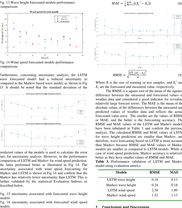
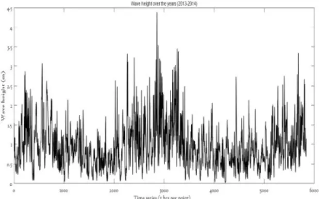
Based on the above analysis, it has been found that both proposed models are effective in weather condition forecasting. In this section, we quantitatively compare the two approaches. The modelled data-driven methods here extended are used to forecast one year of weather data (i.e., 2015), which is then compared with actual yearly data (the historical data) via uncertainty analysis and different model evolution Indexes. For the sake of simplicity and a better understanding of comparative analysis of the proposed methods, forecasted and historical yearly datasets are divided into individual months. By doing this, performance comparison of LSTM and Markov models together with historical data statistically visualised for short-term as well as long term forecast, are shown in Figs. 13 and 14. For wave height forecasting, the LSTM accuracy is better than Markov across the entire range of historical data, see Fig 13.

7 Fig. 13 Wave height forecasted models performance

comparisons

Fig. 14 Wind speed forecasted models performance comparisons

Furthermore, concerning uncertainty analysis, the LSTM wave forecasted model had a reduced uncertainty as compared to the Markov based wave model, as shown in Fig 15. It should be noted that the standard deviation of the

predicted values of the models is used to calculate the error bars for uncertainty analysis. However, in the performance comparison of LSTM and Markov for wind speed prediction, the latter performed better as illustrated in Fig 14. The uncertainty associated with wind speed forecasting for Markov and LSTM is shown in Fig 16 and confirm that the Markov has relatively lower uncertainty than LSTM. This is further validated by the statistical Evaluation Indexes as described below.

Fig. 15 uncertainty associated with forecasted wave height models

Fig. 16 uncertainty associated with forecasted wind speed models

Using Model Evaluation Indexes

Several evaluation indexes can be used to evaluate the performance forecasting models such as the root-mean-squared error (RMSE), normalised mean absolute percentage error (NMAPE), symmetric mean absolute percentage error (sMAPE), mean absolute error (MAE) [32]. To confirm the previous conclusion, here we used RMSE and MAE to appraise the proposed weather forecasting models, expressed as: 𝑀𝐴𝐸 =1 𝑁∑ |(𝑋𝑖 ′_{− 𝑋} 𝑖)| 𝑁 𝑖=1 (8) RMSE = √∑Ni=1(Xi′ − Xi)2 𝑁 (9) Where 𝑁 is the size of training or test samples, and 𝑋𝑖′ and

𝑋𝑖 are the forecasted and measured value, respectively. The RMSE is a square root of the mean of the squared difference between the measured and forecasted values of weather data and considered a good indicator for revealing relatively large forecast errors. The MAE is the mean of the absolute values of the differences between the measured and predicted values of weather data and reflects the actual forecasted value error. The smaller are the values of RMSE or MAE, and the better is the forecasting accuracy. The RMSE and MAE values of the LSTM and Markov models have been tabulated in Table 3 and confirm the previous analysis. The calculated RMSE and MAE values of LSTM for wave height prediction are smaller than Markov, and therefore, wave forecasting based on LSTM is more accurate than Markov because RMSE and MAE values of Markov models are smaller as compared to LSTM models. While in case of wind speed prediction, Markov accuracy is relatively better as they have smaller values of RMSE and MAE.

Table 3. Performance validation of LSTM and Markov model using evaluation metrics

7. Conclusion and Discussion

The importance of weather condition for improving the offshore wind farms accessibility and maintenance will only increase in coming years as more offshore assets are installed. Accurate prediction of weather conditions is useful for planning maintenance activities and thereby increasing operational lifetime and improving offshore turbine availability. The resulting increased revenues will benefit offshore operators in the long term.

Models RMSE MAE

LSTM wave height 0.18 0.13

Markov wave height 0.24 0.18

LSTM wind speed 2.58 1.89

8 Two data-driven methods (LSTM and Markov) have

been proposed for long-term weather forecasting where FINO3 data taken to test and validate the proposed techniques forecasting accuracy. Comparative studies suggest that with specific datasets of FINO3, LSTM performance (in terms of accuracy and uncertainty) it is less effective for wind speed forecasting while relatively better at wave height forecasting, as illustrated in Figs. 13 and 14 and documented in Table 3. One main issue associated with the LSTM network is the training time which increases with the size of training datasets and parameter specifications (e.g., hidden layer and Epochs) and therefore including several years of weather data for training model is challenging and time-consuming, unlike the Markov model.

This research outlines application of data-driven models for weather forecasting; however, the result might be different if proposed data-driven models are tested against different resolution (e.g., 10 minutes, 1 hrs) of datasets. Therefore, next task is to carry out sensitivity analysis of these proposed data-driven models and this is kept for future works.

8. Acknowledgements

This project has received funding from the European Union's Horizon 2020 research and innovation program under grant agreement No. 745625 (ROMEO) (“Romeo Project” 2018). The dissemination of results herein reflects only the author's view, and the European Commission is not responsible for any use that may be made of the information it contains.

9. References

[1] Offshore Wind in Europe Key trends and statistics 2018.

https://windeurope.org/wp-content/uploads/files/about- wind/statistics/WindEurope-Annual-Offshore-Statistics-2018.pdf.

[2] C.A. Irawan, Song X., D. Jones, N. Akbari. Layout optimisation for an installation port of an offshore wind farm. European Journal of Operational Research, 259 (2017), pp. 67-83.

[3] G.L. Garrad Hassan. A guide to UK offshore wind operations and maintenance. Scottish Enterprise and the Crown Estate (2013).

[4] Ioannou, A. Angus, F. Brennan. A lifecycle techno-economic model of offshore wind energy for different entry and exit instances. (2018) Applied Energy, 221 pp. 406-424. [5] J. Caroll, A. McDonald, D. McMillan. Failure rate, repair time and unscheduled O&M cost analysis of offshore wind turbines. Wind Energy, 19 (2016), pp. 1107-1119. doi:

10.1016/j.apenergy.2018.03.143

[6] M.N. Scheu, A. Kolios, T. Fischer, F. Brennan, ‘Influence of statistical uncertainty of component reliability estimations on offshore wind farm availability’, Reliability Engineering and System Safety, Volume 168, December 2017, Pages 28-39.

[7] M. Scheu, D. Matha, M-A. Schwarzkopf, ‘Human Exposure to Motion during Maintenance on Floating Offshore Wind Turbines’, Ocean Engineering, 165, 2018, pp. 293-306.

[8] I.A. Dinwoodie, V.M. Catterson, D. McMillan. Wave height forecasting to improve off-shore access and maintenance scheduling. IEEE power & energy society general meeting (2013).

[9] V.M. Catterson, D. McMillan, I. Dinwoodie, M. Revie, J.Dowell, J. Quigley, et al. An economic impact metric for evaluating wave height forecasters for offshore wind maintenance access. Wind Energy, 19 (2016), pp. 199-212. [10] J.W. Taylor, J. Jeon. Probabilistic forecasting of wave height for offshore wind turbine maintenance. European Journal of Operational Research, 267 (2018), pp. 877-890, 10.1016/j.ejor.2017.12.021.

[11] Mase, H., Yasuda, T., Mori, N., Tom, T., Ikemoto, A., & Utsunomiya, T. (2014). Analysis and forecasting of winds and waves for a floating type wind turbine. Coastal Engineering Proceedings, 1(34), waves.21. doi:

https://doi.org/10.9753/icce.v34.waves.21.

[12] H. Liu, H.-Q. Tian, X.-F. Liang, Y.-F. Li. Wind speed forecasting approach using secondary decomposition algorithm and Elman neural networks. Applied Energy, 157 (2015), pp. 183-194.

[13] F.P. García Márquez, I.P. García-Pardo. Principal component analysis applied to filtered signals for maintenance management. Qual Reliab Eng Int, 26 (2010), pp. 523-527.

[14] N. Aghbalou, A. Charki, S. R. Elazzouzi and K. Reklaoui, "Long Term Forecasting of Wind Speed for Wind Energy Application," 2018 6th International Renewable and Sustainable Energy Conference (IRSEC), Rabat, Morocco, 2018, pp. 1-7. doi: 10.1109/IRSEC.2018.8702892.

[15] G. W. Chang, H. J. Lu, L. Y. Hsu and Y. Y. Chen, "A hybrid model for forecasting wind speed and wind power generation," 2016 IEEE Power and Energy Society General Meeting (PESGM), Boston, MA, 2016, pp. 1-5. doi: 10.1109/PESGM.2016.7742039.

[16] K. R. Nair, V. Vanitha and M. Jisma, "Forecasting of wind speed using ANN, ARIMA and Hybrid models," 2017 International Conference on Intelligent Computing, Instrumentation and Control Technologies (ICICICT),

Kannur, 2017, pp. 170-175. doi:

10.1109/ICICICT1.2017.8342555.

[17] J. Jung, R.P. Broadwater. Current status and future advances for wind speed and power forecasting. Renew Sustain Energy Rev, 31 (2014), pp. 762-777.

[18] S. Hochreiter, J.J. Schmidhuber. Long short-term memory. Neural Comput, 9 (1997), pp. 1-32, 10.1162/neco.1997.9.8.1735.

[19] Z.C. Lipton. A critical review of recurrent neural networks for sequence learning. CoRR (2015), pp. 1-38. doi: 10.1145/2647868.2654889abs/1506.0.

[20] Michael Hauser, Yiwei Fu, Shashi Phoha, Asok Ray. Neural probabilistic forecasting of symbolic sequences with long short-term memory. J Dyn Syst Meas Control-Trans ASME, 140 (8) (2018) 084502.

[21] Erick Lopez, Carlos Valle, Hector Allende. Wind power forecasting based on echo state networks and long short-term memory. Energies, 11 (4) (2018), p. 526, 10.3390/en11030526.

9 [22] Lei J., Liu C., Jiang D. Fault diagnosis of wind turbine

based on Long Short-term memory networks. Renew. Energy, 133 (2019), pp. 422-432.

[23] M. Shafiee. Maintenance logistics organization for offshore wind energy: Current progress and future perspectives. Renewable Energy, 77 (2015), pp. 182-193. [24] FINO3 metrological masts datasets provided by BMU (Bundesministerium fuer Umwelt, Federal Ministry for the Environment, Nature Conservation and Nuclear Safety) and the PTJ (Projekttraeger Juelich, project executing organisation). Available online at https://www.fino3.de/en/. [25] A Beginner’s Guide to Recurrent Networks and LSTMs.

Available online at

https://www.cnblogs.com/hansjorn/p/5398328.html.

[26] X. Chen, X. Lin. Big data deep learning: challenges and perspectives. IEEE Access, 2 (2014), pp. 514-525, 10.1109/ACCESS.2014.2325029.

[27] Hochreiter, S., and J. Schmidhuber. Long short-term memory. Neural computation. Vol. 9, Number 8, 1997, pp.1735–1780.

[28] Long Short-Term Memory Networks, Matlab toolbox. [29] Kulkarni, V. Introduction to Modeling and Analysis of Stochastic Systems. Springer Texts in Statistics; Springer: New York, NY, USA, 2010.

[30] Seyr, H.; Muskulus, M. Decision Support Models for Operations and Maintenance for Offshore Wind Farms: A Review. Appl. Sci. 2019, 9, 278.

[31] Alskaif, T., Schram, W., Litjens, G. and Sark, W. (2017) ‘Smart Charging of Community Storage Units Using Markov Chains’, Innovative Smart Grid Technologies Conference Europe (ISGT-Europe), 2017 IEEE PES, pp. 1–6. doi: 10.1109/ISGTEurope.2017.8260177.

[32] Botchkarev, A. Performance Metrics (Error Measures) in Machine Learning Regression, Forecasting and Prognostics: Properties and Typology. 2018. Available online: https://arxiv.org/abs/1809.03006 (accessed on 20th June 2019).