Robust direct position determination methods in the presence of array model errors

R E S E A R C H

Open Access

Robust direct position determination

methods in the presence of array

model errors

Ding Wang

, Jiexin Yin

, Ruirui Liu

, Zhidong Wu

and Tao Tang

Abstract

Direct position determination (DPD) methods are known to have many advantages over the traditional two-step localization method, especially for low signal-to-noise ratios (SNR) and/or short data records. However, similar to conventional direction-of-arrival (DOA) estimation methods, the performance of DPD estimators can be dramatically degraded by inaccuracies in the array model. In this paper, we present robust DPD methods that can mitigate the effects of these uncertainties in the array manifold. The proposed technique is related to the classical auto-calibration procedure under the assumption that prior knowledge of the array response errors is available. Localization is considered for the cases of both unknown and a priori known transmitted signals. The correspondingmaximum a posteriori (MAP) estimators for these two cases are formulated, and two alternating minimization algorithms are derived to determine the source location directly from the observed signals. The Cramér-Rao bounds (CRBs) for position estimation are derived for both unknown and known signal waveforms. Simulation results demonstrate that the proposed algorithms are asymptotically efficient and very robust to array model errors.

Keywords:Array signal processing, Source localization, Direct position determination (DPD), Array model errors, Alternating minimization algorithm, Cramér-Rao bound (CRB)

1 Introduction

Emitter localization using direction-of-arrival (DOA) measurements [1–3] has received significant atten-tion because of its importance in fields such as radar, sonar, seismology, vehicle navigation, and wireless communications. In this type of localization system, a single moving observer or multiple station-ary observers are used to determine the emitter pos-ition. Generally, each base station is equipped with an antenna array that can be used to estimate the angle of arrival of the transmitted signals. With mul-tiple DOA estimates from different observer loca-tions, it is possible to locate the source [4–6]. This emitter localization procedure is called two-step lo-cation. In the first step, the signal parameters (e.g., DOA [1–6], time difference of arrival (TDOA) [7, 8],

time of arrival (TOA) [9, 10], frequency difference of arrival (FDOA) [11, 12], frequency of arrival (FOA) [13], received signal strength (RSS) [14], gain ratios of arrival (GROA) [15]) are obtained independently from the intercepted signals by spatially separated sensors. In the second step, the measurements of all sensors are transferred to a central unit and the transmitter location is estimated. Note that this two-step procedure is also known as the decentra-lized approach [16].

It is worth mentioning that, although the two-step approach is extensively used in modern localization systems, it is only a suboptimal position determin-ation technique. This is because the signal metrics extracted from the waveforms ignore the constraint that all measurements must correspond to the same transmitter. Consequently, information loss between the two steps is inevitable. Indeed, the extended in-variance principle (EXIP) [17] can be used to show that the two-step procedure can also provide an asymptotically efficient estimate under certain

* Correspondence:[email protected]

1_{National Digital Switching System Engineering and Technological Research}

Center, Zhengzhou 450002, People_’s Republic of China

2_{Zhengzhou Information Science and Technology Institute, Zhengzhou}

450002, Henan, People’s Republic of China

conditions. In practice, however, these requirements are not easily satisfied.

To improve the localization accuracy of two-step location methods, the direct position determination (DPD) technique has been proposed and extensively developed. DPD is a centralized and single-step loca-tion technique in which the estimator uses exactly the same signal samples as in two-step methods, but estimates the source location directly, skipping the intermediate (first) step. This can be viewed as searching for the emitter location that best explains the collected data. In general, the DPD method is superior to the classical two-step methods for low signal-to-noise ratios (SNR) and/or short data re-cords. Moreover, DPD can be applied to many wire-less positioning systems. In particular, DPD methods for locating a narrowband radio emitter based on Doppler shift [18, 19] and for locating a wideband source using a time delay metric [20–22] have been presented. Additionally, DPD estimators using both the Doppler effect and the relative delay have been developed [23–26]. In the DPD methods mentioned above, several platforms each carrying single-antenna receivers are used for source location; hence, the DOA information of the impinging signals cannot be exploited. To use such signal metrics, DPD methods based on multiple static stations, each equipped with an antenna array, have been proposed [27]. This single-step location technique models the array re-sponse as a function of the source position, requir-ing only a two-dimensional search for planar geometry and a three-dimensional search for the general case. Following the methods in [27], other DPD estimators for special localization scenarios have been reported in the literature. Specifically, DPD methods for multiple-source scenarios are stud-ied in [28, 29], and some high-resolution DPD methods are proposed in [30–32]. Additionally, DPD methods tailored to special signal structures (e.g., or-thogonal frequency division multiplexing signals, cyclostationary signals, noncircular signals, and inter-mittent emissions) have been developed [33–37]. Note that the experimental results in [18–37] dem-onstrate that the single-step approach outperforms the two-step method in scenarios with low SNR and/ or relatively few data records.

High-resolution DOA estimation methods are known to be sensitive to errors in the array response model [38–42]. This is because these approaches re-quire exact knowledge of the array manifold. Note that the DPD methods using an antenna array also rely on the accuracy of the array model. As a result, it is reasonable to expect their localization accuracy to deteriorate significantly in the event of an array

model mismatch. In [43–45], for the case of a known signal waveform, the closed-form expression for the mean square error (MSE) of the DPD estima-tor was derived for the case of array model errors. However, in practice, the signal waveform is rarely known. Consequently, an alternative statistical ana-lysis of the DPD method in the presence of array model errors was performed [46] under the assump-tion that the signal waveform is unknown. All the theoretical and experimental results in [43–46] dem-onstrate that the accuracy loss caused by array model errors is considerable. Hence, a new DPD technique that accounts for array model errors is needed to improve the emitter location accuracy. However, to the best of our knowledge, very few studies have considered this topic. This paper pre-sents robust DPD methods that can reduce the im-pact of uncertainties in the array manifold. The proposed technique is similar to the traditional auto-calibration procedure in the field of array signal processing and assumes that certain prior knowledge of the array response errors is available. This is a reasonable assumption in most applications, and it allows for more general perturbation models. We consider two different localization cases: the case of a priori known signal waveforms and the more real-istic case where the transmitted signals are unknown to the location systems. The corresponding maximum a posteriori (MAP) estimators for the two cases are formulated and two alternating minimization algorithms are developed to estimate the emitter position directly from the received signal samples. Hence, the proposed methods follow the Bayesian framework [47–50]. Additionally, to verify the asymptotic efficiency of the new methods, the Cramér-Rao bounds (CRBs) for position estimation are derived for both unknown and known signal waveforms.

The remainder of this paper is organized as fol-lows. Section 2 describes the method and experi-mental used in this paper. In Section 3, the signal model for DPD is formulated and the array error model is also discussed. Section 4 presents a robust DPD method in the presence of array model errors, when signal waveform is unknown. In Section 5, an alternative robust DPD method in the presence of uncertainties in array manifold is proposed for the case of known transmitted signals. In Section 6, the CRB expressions for the position estimation are derived for both unknown and known signal waveforms. Simulation results are reported in Section 7. Conclusions are drawn in Section 8. The proofs of the main results are given in the Appendix

2 Methods/experimental

This study refers to the field of emitter localization. The aim of this study is to propose the robust DPD methods that can mitigate the effects of these uncer-tainties in the array manifold. The methods are de-signed based on MAP criterion. We consider two different localization cases: the case of a priori known signal waveforms and the more realistic case where the transmitted signals are unknown to the location systems. The numerical optimization tech-nology is applied and two alternating minimization algorithms to identify the unknown parameters are presented. To verify the asymptotic efficiency of the new methods, we derive the CRBs on position estimation for both unknown and known signal waveforms.

We perform a set of Monte Carlo simulations to examine the behavior of the proposed robust DPD methods. The root mean square error (RMSE) of position estimate is employed to assess and compare the performance. All the simulation results are aver-aged over 2000 independent runs. We compare our algorithms with the algorithms in [27], and the trad-itional two-step localization algorithms, as well as the CRB for unknown and known signal waveforms. Besides, all the experiments are conducted for the 3D localization.

All data and procedures performed in the paper are in accordance with the ethical standards of re-search community. This paper does not contain any studies with human participants or animals per-formed by any of the authors.

3 Problem formulation

3.1 Signal model for direct position determination 3.1.1 Time-domain signal model

Consider a stationary radio emitter and N base sta-tions that can intercept the transmitted signal. Each base station is equipped with an antenna array com-posed of M sensors. The transmitter’s position is de-noted by an L× 1 vector of coordinates p. In this paper, we consider the three-dimensional (3D) sce-nario, in which p= [px py pz]T and L= 3. The complex envelopes of the signal observed by the nth base station are modeled by

xnð Þ ¼t βnanðp;μnÞs tð−τnð Þp −t0Þ þεnð Þt ð1≤n≤NÞ ð1Þ

where

an(p) is the array response of the nth station to a

signal transmitted from position p,

s(t−τn(p)−t0) is the signal waveform transmitted

at unknown timet0and delayed byτ_n(p),

τn(p) is the signal propagation time from the

emitter to thenth base station (i.e., distance divided

by signal propagation speed),

βn is an unknown complex scalar representing the

channel attenuation between the emitter and the

nth base station,

εn(t) denotes temporally white, circularly symmetric

complex Gaussian noise with zero mean and

covariance matrixσ2

εIM,

μnrepresents the perturbed array parameters and is

used to model the uncertainty in the array steering vector.

We assume that the observation vector xn(t) is sam-pled with period T. The kth data sample can then be expressed as

xn;k ¼βnanðp;μnÞs kTð −τnð Þp −t0Þ þεn;k ð1≤k≤KÞ ð2Þ

whereKis the number of snapshots.

3.1.2 Frequency-domain signal model

In order to determine the emitter position directly from the received signal samples, it is desirable to separate the propagation delay τn(p) and transmit time t0 from the signal waveform. This is easy when using the frequency-domain representation of the problem. Taking the discrete Fourier transform (DFT) of (2), we get

xn;k ¼βnanðp;μnÞsk expf−jωkðτnð Þ þp t0Þg þεn;k

1≤n≤N ; 1≤k≤K

ð Þ

ð3Þ

where

ωk= 2π(k−1)/(KT) is thekth known discrete

frequency point,

sk is thekth Fourier coefficient of the unknown

signal corresponding to frequencyω_k,

εn;k is thekth Fourier coefficient of the random

noise corresponding to frequencyω_k.

As the DFT is an orthogonal linear transformation, the probability distribution of the noise vector εn;k is

Eεn;k

Note that the robust DPD methods proposed in this paper are derived from the frequency-domain signal model (3). For notational convenience, we introduce the following three vectors

3.2 Array error model

This subsection describes the array error model. Ac-cording to the discussion in [47, 48, 50], μn can be modeled by considering it as a real random vector and is composed of the array parameters that are subject to perturbations. A nominal value of μn, de-noted by μn, 0, is known, resulting in a nominal array manifold an(p,μn, 0). As a consequence, the ac-tual array response may be different. We denote the length of μn as Qn.

It is known that μn may include either structured parameters, such as the sensor gain, phase, position, and/or mutual coupling, or unstructured parameters. Generally, the perturbation parameter vector μn can be modeled as a Gaussian random variable with mean E[μn] =μn, 0 and covariance

E μ_n−μ_n;0μ_n−μ_n;0T

¼Ωn ð1≤n≤NÞ ð6Þ

Moreover, μ_n1 and μ_n2 are statistically independent for n1≠n2. Note that the covariance matrices {Ωn}1≤

n≤N are also assumed to be known. These matrices can be determined, for example, using sample statis-tics from a number of independent, identical calibra-tion experiments or using tolerance data specified by the sensor manufacturer [51].

In the next sections, the a priori information in the form of a probability distribution is used to de-velop two robust DPD methods with regard to array model mismatch. The first DPD method covers the common case of signals with unknown waveforms, and the second one is applicable to the less common case of signals with known waveforms. For nota-tional simplicity, we define the following two vectors

μ0¼ μH1;0 μH2;0 ⋯ μHN;0

4 Robust direct position determination method for case of unknown signal waveform

In this section, we propose a new DPD method that is robust to array model errors and assumes that the signal waveforms are unknown. The optimal MAP estimator for the problem at hand is formulated, and a computationally efficient numerical algorithm is derived.

4.1 Optimization criterion for maximum a posteriori estimator

If the transmitted signals are unknown, the parame-ters to be determined involve p, fskg_1≤k≤K, t0, β, and

μ. From (5), both fskg_1≤k≤K and t0 are contained in the vector s. Hence, the estimation of fskg_1≤k≤K and t0can be replaced by the estimation of s.

When deriving the MAP estimator, the a priori distribu-tion of {μn}1≤n≤N must be exploited. Following [47–50],

function, which is given by

JU‐MLðp;s;β;μÞ ¼

where ⊗ denotes Kronecker product, and ⊙

repre-sents Schur product (element by element multiplica-tion), and

γnð Þ ¼ ½p expf−jω1τnð Þpg expf−jω2τnð Þpg ⋯

expf−jωKτnð ÞpgT

ð11Þ

Setting Ωn;0¼Ωn=σ2_ε, the optimization criterion can

min

where we assume, without loss of generality, that the

first element in s is equal to one so that the solution

is unique and unambiguous.

Obviously, (12) is a multidimensional nonlinear minimization problem, and no closed-form solution is available. In the next subsection, we present an ef-ficient numerical algorithm to solve (12). For this purpose, the following matrices are introduced:

f

Recalling (12), it is apparent that the unknown par-ameter vectors of p, s, β, and μ cannot be com-pletely separated. Hence, the straightforward minimization of (12) with respect to p, s, β, andμ is rarely feasible. Because of the diversity of the un-knowns, we derive an alternating minimization algo-rithm to identify the unknown parameters in an iterative manner. This numerical method has been successfully applied to a variety of signal processing issues [52, 53].

After careful analysis of the present problem, the unknown parameters can be grouped into two cat-egories: one is composed of p and s, and the other comprises β and μ. The two sets of variables are al-ternately optimized in succession. First, the minimization is performed with respect to p and s, while β and μ are kept unchanged. Subsequently, we solve the problem for β and μ while keeping p and s

constant. This procedure is repeated until the con-vergence criterion is satisfied. A detailed description of the two steps in each iteration is given in the fol-lowing subsection.

4.2.1 Joint optimization of p ands

First, consider the joint optimization of p and s, with

β and μ given by β^ðaÞ and μ^ðaÞ, respectively. Fortu-nately, when β and μ are fixed, the estimation of p

and s can be decoupled.

Using the result in [27], we have the following optimization problem for finding the position vectorp.

max

where λmax{⋅} denotes the maximal eigenvalue of its

in-put matrix and

imal eigenvalue of some positive semidefinite matrix

and, hence, the functional form of f1(p) with respect

to p is not explicit. The most straightforward

method for solving (15) may be a grid search, as rec-ommended in [27]. However, this method is very computationally expensive when the area of interest is large and the grid step size is small. To avoid a

multidimensional search, we derive an efficient

Gauss-Newton algorithm, which has much faster convergence speed than the steepest ascent and stee-pest descent methods. For this purpose, we first introduce the following proposition, which is associ-ated with the matrix eigenvalue perturbation result.

Proposition 1: Let Z∈Cn×nbe a positive semidefi-nite matrix with eigenvalues λ1≤λ2≤ ⋯ ≤λn, associ-ated with unit eigenvectors v1 , v2 , ⋯ , vn, respectively. Moreover, λjdiffers from the other eigen-values. Assume Z is corrupted by a Hermitian error matrix δΖ∈Cn×n, and the corresponding perturbed matrix is denoted as Z^, i.e., Z^ ¼ZþδZ∈Cnn. If the

the second-order Taylor series expansion of the cost function f1(p), from which the gradient and Hessian matrix of f1(p) can be obtained.

Assume that vector ^p belongs to some neighbor-hood of the true value p. The second-order Taylor series expansion of Cðp^;μ^ðaÞÞ around p leads to

eigenvalues and relevant unit eigenvectors of matrix

Cðp;^μðaÞÞ, respectively. Combining (15), (17), and

Define the following vector and matrices

h p;μ^ð Þa

where the second equality follows from the fact that

f1(⋅) is a real function and δp is a real vector. From

(26), Refhðp;μ^ðaÞÞg and RefHðp;^μðaÞÞg are the

gra-dient and Hessian matrix of f1(p), respectively.

Con-sequently, the Gauss-Newton algorithm for solving (15) is given by

where α∈(0, 1) denotes the step size, and superscript i

indexes theith iteration.

Before proceeding, some remarks are concluded. Remark 1: Clearly, (15) is a nonlinear least-squares optimization problem, so it can be effectively solved by the Gauss-Newton algorithm.

Remark 2: Note that the imaginary parts of hðp;μ^ðaÞÞ

this does not lead to any information loss or perform-ance degradation. The vanishing term in the second equality in (26) is δpT Imfhðp;^μðaÞÞg þδpT ImfHðp;

^

μðaÞ_{Þg δp=}

2 , which is equal to zero because f₁ðp^Þ, f1(p), and δp are real scalars or vectors. As a result, Refhðp;μ^ðaÞÞg and RefHðp;μ^ðaÞÞg are the true gradi-ent and Hessian matrix of f1(p), respectively, and no approximation is necessary. Hence, (27) can be viewed as a standard Gauss-Newton algorithm.

Remark 3: It is worth noting that apart from Gauss-Newton algorithm, there are many other local search algorithms, such as Newton algorithm, stee-pest descent algorithm, Levenberg-Marquardt algo-rithm, etc. However, Newton algorithm is much more computationally demanding because it requires computing the second-order derivative of the cost function; steepest descent algorithm has slower convergence rate than the other algorithms; Levenberg-Marquardt algorithm needs to introduce a reasonable damping factor, which is difficult to de-termine. For these reasons, we use Gauss-Newton al-gorithm to solve (15). In our simulation performed in Section 7, this algorithm can provide satisfactory results. Besides, it must be emphasized that all these algorithms can only guarantee local convergence; that is to say, it is not guaranteed to obtain the glo-bal optimal solution for these algorithms.

Remark 4: In the simulations described in Section

7, the step sizeα is set to 0.85. A number of simula-tion results indicate that this value for α provides good estimates of the source position.

Assuming that the convergence result of (27) is p^ðaÞ, the derivation in [27] implies that the optimal solution ofsis given by

bsð Þa ¼vmax B p^ð Þa;μ^ð Þa

B ^pð Þa;^μð Þa

H

ð28Þ

where vmax{⋅} denotes the eigenvector (with first

element equal to one) corresponding to the largest eigenvalue of its matrix argument.

4.2.2 Joint optimization ofβandμ

This subsection describes the minimization of the criter-ion in (12) with respect to β and μ, while p and s are

fixed at^pðaÞandbsðaÞ, respectively.

Likewise, the estimation of β and μ can also be decoupled. First, the channel attenuation scalar {βn}1≤

n≤Nthat minimizes (12) is given by

^ βn;opt¼

1

an p^ð Þa;μn

2

2

bsð Þa⊙γ_n ^pð Þa

2

2 bsð Þa⊙γ_n ^pð Þa

an ^pð Þa;μn

H

xn

1≤n≤N

ð Þ

ð29Þ

Inserting (29) back into (12) we get the following con-centrated problem

As each term in the sum only depends on the par-ameter of one array (i.e., μn), the minimization in (30) can be performed by solving the following N subproblems:

where

Obviously, (31) is a nonlinear least-squares optimization problem, which can be efficiently solved by the Gauss-Newton algorithm. The corresponding iterative formula is given by

where i is the iteration number and Gn(μn) is the Jacobian matrix ofgn(μn), i.e.,

Gnð Þ ¼μn

∂g_nð Þμ_n

∂μT

n

¼ Gn;1ð Þμn

Gn;2ð Þμn

ð34Þ

Gn;1ð Þ ¼μn

We conclude some remarks as follows.

Remark 5: Similarly, as (31) is also a nonlinear least-squares optimization problem, we can use the Gauss-Newton algorithm to find its optimal solution.

Remark 6: The imaginary parts of ðGnð^μð_niÞÞÞHGnð^μð_niÞÞ

and are neglected

in (33). Nevertheless, this does not mean that there are any approximations in (33), because μn is a real vector. The detailed derivation of (33) is given in

Appendix 2.

Assuming that the convergence result of (33) is ^μð_naÞ, substituting this back into (29) leads to the estimation

of β, which is denoted byβ^ðaÞ.

4.2.3 Summary of the alternating minimization algorithm

The ingredients of the previous two subsections can be combined to form the proposed alternating minimization algorithm, which is summarized as follows.

Proposed alternating minimization algorithm I

Step 1: Define a convergence thresholdδ> 0 and choose the initial valuesp^ð0Þ,^sð0Þ,^μð0Þandβ^ð0Þ.

Step 2: Set the iteration counterm≔0 and compute the cost function Jð_UmÞusing (12).

Step 3: Calculatep^ðmÞusing the Gauss-Newton algorithm given in (27).

Step 4: Compute^sðmÞaccording to (28).

Step 5: Calculateμ^ðmÞfrom (33).

Step 6: Compute^βðmÞvia (29).

Step 7: Increment the iteration counterm≔m+ 1 and compute the cost functionJðUmÞusing (12). IfjJ

ðmÞ

U −J

ðm−1Þ

U j≤δ, stop the procedure; otherwise go to Step 3.

The following remarks concern the alternating minimization algorithm described above.

Remark 7: The algorithm iterates until the convergence criterion is satisfied. Similar to the analysis in [54], it follows that, at each step, the cost function reduces so that Jð_U1Þ>J_Uð2Þ>⋯> Jð_UmÞ≥0 . Therefore,

fJð_UmÞgþ_m∞_¼1 is a convergent series and the convergence is ensured. Based on our experimental results, 20 iterations are sufficient to guarantee the convergence.

Remark 8: As in many iterative algorithms, convergence to the global optimum of the cost function depends on the initial estimate. If the initial values are properly chosen, the effects of these initial errors can largely be removed. For the problem at hand, the initial value ofμ can be chosen as its nominal value μ0, and the starting point ofpcan be obtained using the traditional two-step localization method, where the DOA parameter can be es-timated by subspace-based methods [1–3]. If the un-knowns to be found are DOAs, the array manifold in (1)-(3) should be modeled as a function of direction, as in [1–3]. This is not difficult, because the position vectorpis a function of direction. Once the DOAs relative to all ar-rays have been estimated, the initial source position can be easily determined using the closed-form method [4]. In addition,sandβcan be initialized from (28) and (29), re-spectively. The simulation results in Section 7 demon-strate that using these initial estimates gives satisfactory performance.

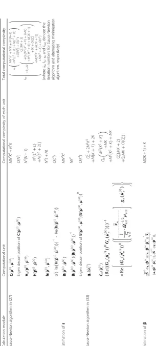
4.2.4 Complexity analysis

Here, the computational complexity of the proposed DPD method is studied in terms of the number of multiplication. Table1summarizes the numerical complexity.

5 Direct position determination method for case of known signal waveform

array manifold for the case of known signal waveforms. Applications of this study can be found in, for example, wireless communications, where some known preamble sequences are often transmitted for training or synchronization purposes [55, 56]. Similar to Section 4, the robust DPD algorithm developed here is also based on an optimal MAP estimator for the current problem.

5.1 Optimization criterion for maximum a posteriori estimator

If the transmitted signals are a priori known, the sole unknown parameter embedded in s is t0. Consequently, we can consider the estimation oft0instead of s. Using the a priori distribution of {μn}1≤n≤N, the MAP estimator function for the case of known waveform, which can be formulated as

Note that the vector s0 is known here. Combining (37)–(39), we obtain the following optimization problem:

It does not seem possible to solve (41) in closed form because of its nonlinear nature. In the next subsection, an efficient numerical algorithm for solving this problem is presented.

5.2 Numerical algorithm

The algorithm proposed in this subsection is similar to that in Subsection 4.2, and is also implemented by adopting the alternating minimization algorithm. After a close inspection of (41), we can divide the unknown parameters into two categories: one is composed of p

andt0, and the other comprisesβandμ. The two sets of variables are alternately updated by separate optimization procedures. A detailed description of the proposed algorithm is given in the following subsections.

5.2.1 Joint optimization of p and t0

We perform joint optimization with respect top andt0, withβandμfixed to^βðbÞ and^μðbÞ, respectively.

According to the derivation in [27], the joint estimates of p and t0 can be obtained by solving the following optimization problem:

We define a permutation matrixΠsubject to

vec B p;μ^ð Þb can then be written as

First, we consider t0 as a nuisance parameter and rewrite (45) as an optimization problem for the position vectorpas follows:

max Therefore, the most straightforward method for solving (46) may be a grid search. However, this is computationally intensive, as stated previously. Thus, we develop an iterative algorithm for solving (44) based on the Gauss-Newton algorithm.

To obtain an iterative procedure, we need to derive the gradient and Hessian matrix of the cost function f4(p). For this purpose, a preliminary mathematical result is presented as follows.

Proposition 2: Consider a twice continuously

differentiable function f(z,y) that depends on the independent variables y∈R and z∈Rm× 1. Define a

The proof of Proposition 2 is provided in

Appendix 3. Note that the gradient and Hessian

matrix of the criterion function f4(p) can be obtained from this result.

We first assume that, for a given p, the point that maximizes f3(p,t0) with respect to t0 is denoted as t0, m(p). This can be obtained by the fast Fourier transform

(FFT) [27]. Using (45) and the first equality in (48), the

Furthermore, using the second equality in (48), the Hessian matrix of f4(p) can be formulated as

Combining (45) and (50) leads to

At this point, the Gauss-Newton algorithm for solving (46) can be formulated as

^ represents the iteration number.

Let the convergence result of (56) be p^ðbÞ. Then, t0 can be obtained from the following minimization problem:

Note that the cost function in (57) can be minimized via FFT algorithm, which has been discussed in [27].

5.2.2 Joint optimization ofβandμ

The objective function in (41) is now minimized with respect toβ andμ, withp and t0given by ^pðbÞ and^t

ðbÞ 0 ,

respectively. Note that the algorithm presented in Section4.2.2 can still be applied here, but p^ðaÞ, γ_nð^pðaÞÞ,

5.2.3 Summary of the alternating minimization algorithm

A possible implementation of the proposed alternating minimization algorithm is outlined as follows.

Proposed alternating minimization algorithm II

Step 1: Define a convergence thresholdδ> 0 and choose the initial valuesp^ð0Þ,^tð₀0Þ,^μð0Þand^βð0Þ.

Step 2: Set the iteration counterm≔0 and compute the cost function Jð_KmÞusing (41).

Step 3: Calculatep^ðmÞusing the Gauss-Newton algorithm given in (56).

Step 4: Compute^tð₀mÞfrom (57) by FFT algorithm.

Step 5: Calculateμ^ðmÞfrom (33) and (58).

Step 6: Compute^βðmÞvia (29) and (58).

Step 7: Increment the iteration counterm≔m+ 1 and compute the cost functionJðKmÞusing (41). IfjJ

ðmÞ

K −J

ðm−1Þ

K j≤δ, stop the procedure; otherwise go to Step 3.

In the following, we make two remarks concerning the alternating minimization algorithm described above.

Remark 9: Similar to sequencefJð_UmÞgþ_m∞_¼1,fJð_KmÞgþ_m∞_¼1 is also monotonically decreasing and, hence, convergence is guaranteed. From our simulation results, it can be observed that 20 iterations are generally enough to satisfy the convergence criterion.

Remark 10: The selection of the initial values is again important. For the current problem, the initial value of μ can be chosen as its nominal value μ0 and the starting point of p can be obtained using the two-step localization method, where the DOA param-eter can be estimated by the algorithm proposed for the scenario of known waveforms [55, 56]. As stated in Remark 8, when the unknowns to be determined are DOAs, we need to express the array manifold in (1)–(3) as a function of direction, as in [1–3]. This can easily be achieved, because the position vector p

is a function of DOA. Once the DOAs corresponding to all the arrays have been estimated, the estimated initial position is given by the closed-form method

[4]. Further, from (57), we have the initial solution of t0 from the FFT algorithm, and the initial guess of β can be given by (29) and (58). From the results in Section 7, it is clear that these initial estimates allow the proposed algorithm to provide satisfactory estimation accuracy.

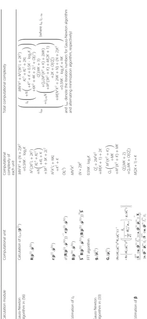
5.2.4 Complexity analysis

We now address the computational complexity of the proposed DPD method in terms of the number of multiplications. Table 2 summarizes the numerical complexity.

6 Cramér-Rao bound on covariance matrix of localization errors

The CRB gives a lower bound on the asymptotic covariance matrix of any asymptotically unbiased estimator. The bound can be obtained by the inverse of the Fisher information matrix (FIM). Relating the parameter estimates to this bound can provide a nature measure of performance. The purpose of this section is to derive the CRBs for the estimates of the emitter’s position. We consider the cases when the signal waveform is unknown and when the signal waveform is known.

6.1 Cramér-Rao bound on position estimate for case of unknown signal waveform

This subsection is devoted to the derivation of the CRB for localization under the assumption that the signal waveform is unknown. For this case, the full parameter set contains both the deterministic parametersσ2

ε,p,β,s

, and the stochastic parameter μ. Hence, the CRB derivation should follow the Bayesian theory framework [47–50]. Note that the CRB derivation can also be used for stochastic parameters, as in [47–50, 57, 58]. To this end, a novel parameter vector that comprises all the deterministic and stochastic unknowns is introduced as

ηð Þa _{¼ σ}2

We proceed to define a data vector as

x¼xH₁ xH₂ ⋯ xH_NH

¼ ½xH_1;1 xH_1;2 ⋯ xH_1;K xH_2;1 xH_2;2

⋯ xH_2;K ⋯ ⋯ xH_N;1 xH_N;2

⋯ xH_N;KH

ð61Þ

The mean vector ofxis given by

x0¼E½ ¼ ½x xH1;1;0 xH1;2;0 ⋯ xH1;K;0 xH2;1;0 xH2;2;0

When the deterministic and stochastic parameters coexist, we should use the hybrid CRB. As a consequence, the FIM for vectorη(a)is given by [47–50,

Ex;μ

so we can still obtain an asymptotically valid CRB. Another reason for ignoring this approximation is that the distribution ofμis symmetric and, in this paper, the errorμ−μ0is assumed to be sufficiently small.

Combining (64) and the above discussion, the FIM for vectorη′(a)can be approximately expressed as

<FIM η0ð Þa

It follows from (67) that

FIM η0ð Þa

Using (62) and (63), and after some algebraic manipulations, the sub-matrices in (68) can be written as

Substituting (68) and (70) into (69) leads to

where

The details of calculating the matrices in (72) are shown inAppendix 4.

Note that, in practice, only the p corner of the CRB matrix is of interest. Invoking the partitioned matrix inversion formula, the CRB matrix for position vector p

can be written as

CRBð Það Þ ¼p σ

Note that the superscript“a”in (73) indicates that this CRB corresponds to the case of an unknown signal waveform. In addition, the trace of this CRB matrix is the minimum achievable localization MSE.

6.2 Cramér-Rao bound on position estimate for case of known signal waveform

In this subsection, the CRB on the covariance matrix of location estimation is deduced for the case where the transmitted signals are a priori known. Accordingly, the complete parameter set comprises the deterministic parameters σ2_ε , p, β, and t0, as well as the random parameter μ. Hence, the hybrid CRB should also be considered. To proceed, we collect all these parameters into the following vector:

ηð Þb _{¼ σ}2 nominal value μ0. According to the analysis in Subsection 6.1, we can still obtain an asymptotically valid CRB. In addition, all the sub-matrices in (77) are given explicitly in (70), except for Tt0. Therefore, we need only derive an expression for Tt0. From (62) and (63), it can be checked that

Tt0 ¼

and (78) into (76) produces

where

(80)

In Appendix 5, the details of calculating the matrices

in (80) are provided.

With the application of the partitioned matrix inversion formula, the CRB matrix for position vector p

can be expressed as

CRBð Þbð Þ ¼p σ

where the superscript “b” indicates the case of a known signal waveform, and the trace of CRB(b)(p) is the minimum achievable MSE for any unbiased localization method.

7 Simulation results

This section presents a set of Monte Carlo simulations to examine the behavior of the proposed robust DPD methods. The RMSE of position estimate is employed to assess and compare the performance. All the simulation results are averaged over 2000 independent runs. We compare our algorithms with the algorithms in [27], and the traditional two-step localization algorithms, as well as the CRB for un-known and un-known signal waveforms. Besides, all the experiments are conducted for the 3-D localization.

7.1 Simulation results for case of unknown signal waveform

In this subsection, the algorithm presented in Section4

is evaluated and its estimation accuracy is compared with that of the first algorithm in [27], which assumes the signal waveform is unknown. Both of these algorithms are denoted as algorithm I in the figures below. In addition, the two-step localization algorithm used for comparison here is realized using the robust Bayesian algorithm [48] to estimate the DOAs in the first step and exploiting the Taylor series (TS) algo-rithm [59] to locate the source in the second phase. If the unknowns to be found are DOAs, the array mani-fold in (1)–(3) should be modeled as a function of dir-ection, as in [1–3]. This is not difficult to achieve because position vector p is a function of direction. The array model mismatch considered here is caused by sensor location perturbations. The sensor position errors are zero-mean Gaussian random variables in both the x and y directions, and are independent and identically distributed (IID) from sensor to sensor and array to array. The standard deviation of the position errors is denoted byσL.

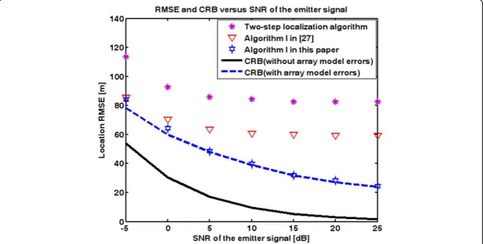
In the first set of experiments, we consider three base stations placed at [0, 2500, 0] m, [0, 0, 0] m, and [0, −2500, 0] m and a single emitter located at [1500, 2000, 2000] m. The transmitted waveforms are realizations of a narrowband Gaussian random process, and are unknown to the receivers. Each base station is equipped with a uniform circular array (UCA). The channel attenuation magnitude is fixed at 1, and the channel phase is selected at random from

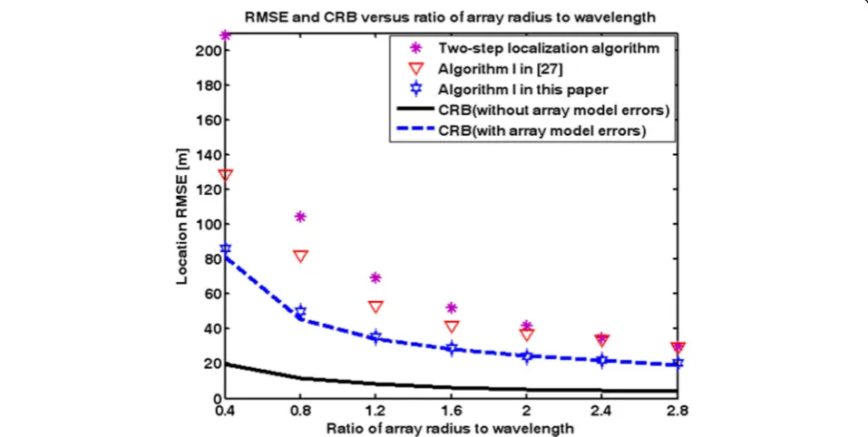
a uniform distribution over [−π, π). Additionally, unless stated otherwise, we use the following settings: (1) K= 128 samples; (2) SNR = 10 dB; (3) M= 5 sensors; (4) σL= 0.03λ (where λ is the wavelength of the carrier signal); and (5) array radius equal to the wavelength. Figures 1, 2, 3, 4, and 5 display the RMSEs of the localization methods as functions of the SNR of the emitter signal, number of snapshots K, standard deviation of the sensor position errors σL, number of array elements M, and ratio of array radius to wavelength, respectively.

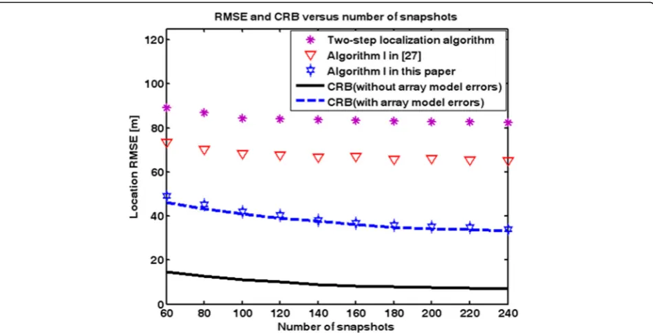
It can be observed from Figs. 1, 2, 3, 4, and 5 that algorithm I in this paper outperforms algorithm I in [27] in terms of the estimation accuracy. The performance gap is especially noticeable for high SNRs and large sensor position errors. This is because, in these cases, the array model errors dominate the performance. Our technique accounts for these errors and incorporates the prior statistics of the array perturbations for source localization. The results in Figs.1, 2,3, 4, and5 show that, when the SNR decreases and the array aperture increases, the proposed algorithm gives only a minor performance improvement. This is because, for lower SNRs and large array apertures, the measurement noise is the dominant error source, and the two algorithms give similar performance. In addition, the estimation accuracy of our algorithm achieves the CRB provided by (73) at moderate noise and error levels. Finally, it is worth noting that the DPD estimators perform significantly better than the two-step localization method. This improvement has been explained in the literature.

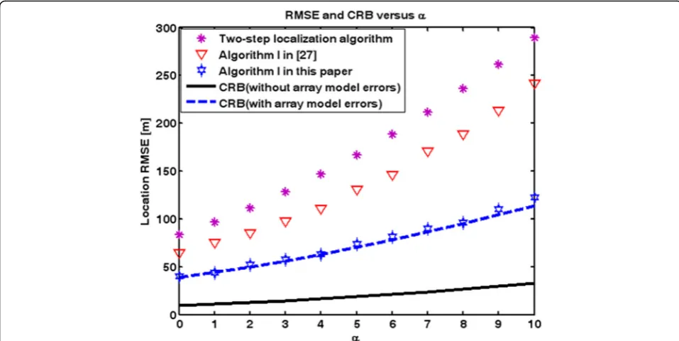
In the second experiment, we use the same simulation settings with a varying emitter location. The source coordinate is set as [1500, 2000, 2000] +α∙[200, 200, 200] m, where α ranges from 0 to 10. The distance between the emitter and the receivers increases as α increases. Figure 6

illustrates the RMSEs of the localization methods with respect to α.

From Fig. 6, we can draw similar conclusions similar to those for Figs. 1, 2, 3, 4, and 5; they are not repeated here for reasons of brevity. We only emphasize that the RMSE improvement from algorithm I in this paper over algorithm I in [27] is more significant as α increases. Hence, the gain in localization accuracy of our algorithm increases as the source moves farther away from the receivers.

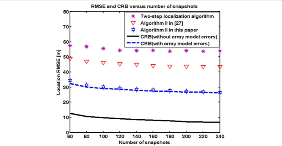
Fig. 2RMSEs of localization methods and the corresponding CRBs as a function of number of snapshots for case of unknown signal waveform

7.2 Simulation results for case of known signal waveform

In this subsection, the positioning accuracy of the algorithm given in Section 5 is compared with that of the second algorithm given in [27], which assumes the signal waveform is known. These are referred to as algorithm II in the following figures. Additionally, for a fair comparison, in the simulated two-step localization

algorithm, the DOAs are estimated by the algorithm pre-sented in [56], which assumes a known waveform. As stated above, when the unknowns to be determined are DOAs, we need to express the array manifold in (1)–(3) as a function of direction, following [1–3]. This can be easily achieved because position vectorpis a function of DOA. The array model error results from sensor gain

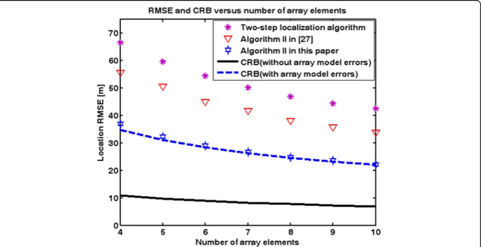
Fig. 4RMSEs of localization methods and the corresponding CRBs as a function of number of array elements for case of unknown signal waveform

and phase uncertainties, corresponding to case 2 in Sec-tion 4 of [39]. Moreover, both gain and phase perturba-tions are independent and identically distributed zero-mean Gaussian random variables. The standard de-viations of the gain and phase errors are denoted asσG and σP, respectively. We assume σG= 0.01σP hereafter; thus, ifσPchanges,σGalters accordingly.

In the first set of experiments, the location system consists of three base stations located at [500, 2500, 0] m, [0, 0, 0] m, and [500, −2500, 0] m. The emitter is positioned at [1500, 500, 2500] m. The signal waveforms are generated in the same way as described in Subsection

7.1, but they are known to the receivers. Each base station is equipped with a UCA. The channel attenuation magnitude is fixed at 1, and the channel phase is selected at random from a uniform distribution over [−π, π). Additionally, unless otherwise specified, we adopt the following simulation parameters: (1) K= 128 samples; (2) SNR = 10 dB; (3) M= 6 sensors; (4) σP= 0.1rad; and (5) array radius equal to wavelength. Figures7,8,9,

10, and 11 plot the RMSEs of the localization methods against the SNR of the emitter signal, number of snapshots K, standard deviation of the sensor phase errors σP, number of array elements M, and ratio of array radius to wavelength, respectively.

In Figures 7, 8, 9, 10, and 11, the RMSEs clearly demonstrate the superior performance of algorithm II in this paper over algorithm II in [27] and the two-step localization algorithm. Moreover, the performance im-provement is more pronounced as the SNR and sensor model errors increase and the array aperture decreases.

The impact of array model mismatch is effectively miti-gated by our algorithm. Additionally, the proposed algo-rithm yields a solution that attains the CRB accuracy provided by (81) at moderate noise and error levels.

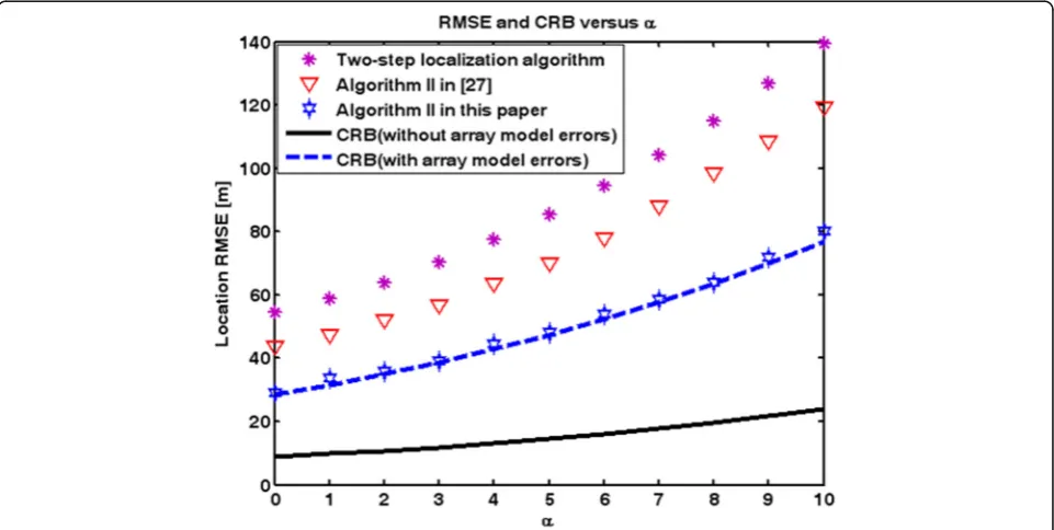
In the second experiment, the same simulation parameters are used, but the source location changes. The emitter position coordinates are set as [1500, 500, 2500] +α∙[200, 200, 200] m, whereαvaries from 0 to 10. Again, the source becomes farther away from the receivers as α increases. Figure12 shows the RMSEs of the localization methods with respect toα.

The performance gain of the proposed algorithm over the other algorithms is corroborated by the results in Fig. 12. Moreover, the RMSE improvement of the new algorithm over algorithm II in [27] becomes stronger as the source moves farther away from the receivers. This observation is consistent with the results in Fig.6.

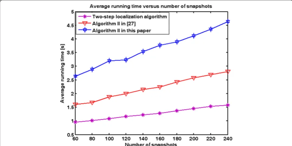
7.3 Running time of the localization methods

In this subsection, the runtime of all the localization methods considered in the experiments is compared. All the simulations were implemented using MATLAB R2016b on a ThinkPad laptop equipped with Intel Core i7–7500 CPU and 8 GB RAM.

First, we adopt the simulation settings used to produce Fig. 2. Figure 13 depicts the average runtime of the considered localization methods as a function of snapshot number. Second, the simulation parameters used to produce Fig. 8 were applied. In Fig. 14, the average runtime versus the snapshot number is compared for the considered localization methods.

It is easily observed from Figs. 13 and 14 that the runtime of the proposed DPD methods is significantly higher than that of the other methods. This is because the model errors are considered and there are too many nuisance variables to be optimized besides the source position vector. The two-step localization method has the fastest runtime

among the compared methods, mainly because it is a decentralized method.

8 Discussion

From the simulation results described above, we can observe that the proposed algorithms can effectively mitigate the effects of array model mismatch, and they

Fig. 8RMSEs of localization methods and the corresponding CRBs as a function of number of snapshots for case of known signal waveform

outperform the algorithms in [27] obviously for high SNRs and large sensor position errors. Moreover, the gain in localization accuracy of our algorithms increases as the source moves farther away from the receivers. The estimation performance of the developed algorithms can

attain the corresponding CRB at moderate noise and error levels. However, the complexity of the proposed algorithms are higher than that of the algorithms in [27] because they account for the array model errors and require more computational procedure. Finally, it needs to be mentioned

Fig. 10RMSEs of localization methods and the corresponding CRBs as a function of number of array elements for case of known signal waveform

that the present study only deals with the single-source situation. In our future work, we intend to extend the pro-posed methods to the multiple-source scenario.

9 Conclusions

This paper presents robust DPD methods that can reduce the negative effect of array model mismatch.

The idea behind the newly proposed technique is similar to that of the array error auto-calibration methods, which assume that certain prior statistical distribution of the array model errors is available. We consider two different localization cases, the case of a priori known signal waveform and the more realistic case where transmitted signals are unknown to the

Fig. 12RMSEs of localization methods and the corresponding CRBs as a function ofαfor case of known signal waveform

location systems. The corresponding MAP estimators for the two cases are formulated and two effective al-ternating minimization algorithms are developed to locate the source directly from the signals captured at several antenna arrays simultaneously. The proposed methods follow the Bayesian framework given in [47– 50]. Besides, for the purpose of verifying the

asymptotic efficiency of the new methods, the CRB expressions for position estimation are also deduced for both unknown and known signal waveforms. Simulation results confirm that the proposed algo-rithms are able to provide the CRB accuracy and the effect of array model errors can be decreased considerably.

Fig. 14Average running time as a function of the snapshot number (the second simulation results)

10 Appendix 1

10.1 Proof of Proposition 1

Assume the normalized eigenvectors of matrixZ^ are^v1 ;

^

v2 ; ⋯ ; ^vn . Applying the Hermitian matrix

eigen-perturbation theory [60], we have

^

ji are the second-order perturbation terms,

i.e., δλð_j2Þ¼OðkδZk2₂Þ and ξð_ji2Þ¼OðkδZk2₂Þ. It follows from the matrix eigen-equation that

^

Comparing the first-order perturbation terms between both sides of (83), it can be observed that

Xn

Furthermore, comparing the second-order perturb-ation terms between both sides of (83), it follows that

Xn

Combining (82), (85) and (87) completes the proof.

11 Appendix 2

11.1 Proof of (33)

Assume that μ^ð_niÞ is the estimation of μn at the ith iteration step. In order to obtain the updated estimate of

μn at the (i+ 1)th iteration, we need to substitute the first-order Taylor series expansion of gn(μn) round μ^ðniÞ

into (31), which yields

(89) It is obvious that (89) is a linear least-squares estima-tor, and its optimal solution satisfies

(90) which indicates that (33) holds true.

12 Appendix 3

12.1 Proof of Proposition 2

From the definition ofym(z), it follows that

On the other hand, using the definition ofym(z) again, we have

Substituting (94) into (92) proves the first equality in (48). Taking the derivative with respect to z on both sides of (94) yields

€f21ðz;ymð ÞzÞ þ€f22ðz;ymð Þz Þ

The second equality in (48) can be proved by inserting (94) and (96) into (93). At this point, the proof of Proposition 2 is completed.

13 Appendix 4

13.1 Detailed derivation of matrices in (72)

It can be seen from (72) that, in order to calculate matri-ces Zð₁aÞ, Z₂ðaÞ, and Zð₃aÞ, we must derive the explicit

TH_{Ref gs}TRef gs ¼

14.1 Detailed derivation of matrices in (80)

From (80) and the results inAppendix 4, in order to cal-culate matricesZð₁bÞ,Z₂ðbÞ, andZð₃bÞ, we need to derive the

Combining (70) and (78) and after some algebraic ma-nipulation, we get

3D:Three-dimensional; CRB: Cramér-Rao bound; DFT: Discrete Fourier transform; DOA: Direction-of-arrival; DPD: Direct position determination; EXIP: Extended invariance principle; FDOA: Frequency difference of arrival; FFT: Fast Fourier transform; FIM: Fisher information matrix; FOA: Frequency of arrival; GROA: Gain ratios of arrival; IID: Independent and identically distributed; MAP: Maximum a posteriori; ML: Maximum likelihood; MSE: Mean square error; RMSE: Root-mean-square-error; RSS: Received signal strength; SNR:

Signal-to-noise ratios; TDOA: Time difference of arrival; TOA: Time of arrival; TS: Taylor series; UCA: Uniform circular array

Acknowledgements

The authors would like to thank the Editorial board and the Reviewers for considering and revising this manuscript. The authors also thank Stuart Jenkinson, PhD, from Liwen Bianji, Edanz Group China (www.liwenbianji.cn/ ac), for editing the English text of a draft of this manuscript.

Funding

This work is supported from National Natural Science Foundation of China (Grant No. 61201381, No. 61401513 and No.61772548), China Postdoctoral Science Foundation (Grant No. 2016M592989), the Self-Topic Foundation of Information Engineering University (Grant No. 2016600701), and the Outstanding Youth Foundation of Information Engineering University (Grant No. 2016603201).

Availability of data and materials

The datasets generated and/or analyzed during the current study are not publicly available but are available from the corresponding author on reasonable request.

Authors_’contributions

DW and JY wrote the manuscript and RL helped with writing and theoretical derivation. ZW and TT were in charge of the experiment and its results. All authors had significant contribution on the development of early ideas and design of the final algorithms. All authors read and approved the final manuscript.

Ethics approval and consent to participate

All data and procedures performed in paper were in accordance with the ethical standards of research community. This paper does not contain any studies with human participants or animals performed by any of the authors.

Consent for publication

Informed consent was obtained from all authors included in the study.

Competing interests

The authors declare that they have no competing interests.

Publisher’s Note

Springer Nature remains neutral with regard to jurisdictional claims in published maps and institutional affiliations.

Received: 4 September 2017 Accepted: 28 May 2018

References

1. RO Schmidt, Multiple emitter location and signal parameter estimation[J]. IEEE Trans. Antennas Propag.34(3), 267_–280 (1986).

2. P Stoica, A Nehorai, MUSIC, maximum likelihood, and Cramér-Rao bound[J]. IEEE Trans. Acoust. Speech Signal Process.37(5), 720–741 (1989). 3. M Viberg, B Ottersten, Sensor array processing based on subspace fitting[J].

IEEE Trans. Signal Process.39(5), 1110_–1121 (1991).

4. SC Nardone, ML Graham, A closed-form solution to bearings-only target motion analysis[J]. IEEE J. Ocean. Eng.22(1), 168–178 (1997).

5. D Kutluyil, Bearings-only target localization using total least squares[J]. Signal Process.85(9), 1695_–1710 (2005).

6. Z Lin, T Han, R Zheng, M Fu, Distributed localization for 2-D sensor networks with bearing-only measurements under switching topologies[J]. IEEE Trans. Signal Process.64(23), 6345–6359 (2016).

7. L Yang, KC Ho, An approximately efficient TDOA localization algorithm in closed-form for locating multiple disjoint sources with erroneous sensor positions[J]. IEEE Trans. Signal Process.57(12), 4598–4615 (2009). 8. W Jiang, C Xu, L Pei, W Yu, Multidimensional scaling-based TDOA localization

scheme using an auxiliary line[J]. IEEE Signal Process Lett.23(4), 546_–550 (2016). 9. KW Cheung, HC So, YT Chan, Least squares algorithms for

11. KC Ho, X Lu, L Kovavisaruch, Source localization using TDOA and FDOA measurements in the presence of receiver location errors: analysis and solution[J]. IEEE Trans. Signal Process.55(2), 684–696 (2007). 12. G Wang, Y Li, N Ansari, A semidefinite relaxation method for source

localization using TDOA and FDOA measurements[J]. IEEE Trans. Veh. Technol.62(2), 853–862 (2013).

13. J Mason, Algebraic two-satellite TOA/FOA position solution on an ellipsoidal earth[J]. IEEE Trans. Aerosp. Electron. Syst.40(7), 1087–1092 (2004). 14. KC Ho, M Sun, An accurate algebraic closed-form solution for energy-based

source localization[J]. IEEE Trans. Audio Speech Lang. Process.15(8), 2542_– 2550 (2007).

15. KC Ho, M Sun, Passive source localization using time differences of arrival and gain ratios of arrival[J]. IEEE Trans. Signal Process.56(2), 464_–477 (2008). 16. M Wax, T Kailath, Decentralized processing in sensor arrays[J]. IEEE Trans.

Signal Process.33(4), 1123–1129 (1985).

17. P Stoica, On reparametrization of loss functions used in estimation and the invariance principle[J]. Signal Process.17(4), 383–387 (1989).

18. A Amar, AJ Weiss, Localization of narrowband radio emitters based on Doppler frequency shifts[J]. IEEE Trans. Signal Process.56(11), 5500_–5508 (2008). 19. D Wang, Y Wu, Statistical performance analysis of direct position

determination method based on doppler shifts in presence of model errors[J]. Multidim. Syst. Sign. Process.28(1), 149–182 (2017).

20. E Tzoreff, AJ Weiss, Expectation-maximization algorithm for direct position determination. Signal Process.97(4), 32_–39 (2017).

21. N Vankayalapati, S Kay, Q Ding, TDOA based direct positioning maximum likelihood estimator and the Cramer-Rao bound[J]. IEEE Trans. Aerosp. Electron. Syst.50(3), 1616–1634 (2014).

22. W Xia, W Liu, LF Zhu, Distributed adaptive direct position determination based on diffusion framework[J]. J. Syst. Eng. Electron.27(1), 28_–38 (2016). 23. AJ Weiss, Direct geolocation of wideband emitters based on delay and

Doppler[J]. IEEE Trans. Signal Process.59(6), 2513–5520 (2011).

24. M Pourhomayoun, ML Fowler, Distributed computation for direct position determination emitter location[J]. IEEE Trans. Aerosp. Electron. Syst.50(4), 2878–2889 (2014).

25. O Bar-Shalom, AJ Weiss, Emitter geolocation using single moving receiver[J]. Signal Process.94(12), 70–83 (2014).

26. JZ Li, L Yang, FC Guo, WL Jiang, Coherent summation of multiple short-time signals for direct positioning of a wideband source based on delay and Doppler[J]. Digital Signal Process.48(1), 58–70 (2016).

27. AJ Weiss, Direct position determination of narrowband radio frequency transmitters[J]. IEEE Signal Process Lett.11(5), 513–516 (2004).

28. AJ Weiss, A Amar, Direct position determination of multiple radio signals[J]. EURASIP J Appl. Signal Process.2005(1), 37_–49 (2005).

29. A Amar, AJ Weiss, A decoupled algorithm for geolocation of multiple emitters[J]. Signal Process.87(10), 2348–2359 (2007).

30. T Tirer, AJ Weiss, High resolution direct position determination of radio frequency sources[J]. IEEE Signal Process Lett.23(2), 192–196 (2016). 31. L Tzafri, AJ Weiss, High-resolution direct position determination using

MVDR[J]. IEEE Trans. Wireless Commun.15(9), 6449–6461 (2016). 32. T Tirer, AJ Weiss, Performance analysis of a high-resolution direct position

determination method[J]. IEEE Trans. Signal Process.65(3), 544–554 (2017). 33. O Bar-Shalom, AJ Weiss, Efficient direct position determination of

orthogonal frequency division multiplexing signals[J]. IET Radar Sonar Navig.

3(2), 101_–111 (2009).

34. AM Reuven, AJ Weiss, Direct position determination of cyclostationary signals[J]. Signal Process.89(12), 2448–2464 (2009).

35. JX Yin, W Ying, W Ding, Direct position determination of multiple noncircular sources with a moving array[J]. Circuits Syst. Signal Process. 2017;36(10):4050-76.

36. JX Yin, W Ding, W Ying, XW Yao, ML-based single-step estimation of the locations of strictly noncircular sources[J]. Digital Signal Process.69(10), 224–236 (2017). 37. M Oispuu, U Nickel, Direct detection and position determination of multiple

sources with intermittent emission[J]. Signal Process.90(12), 3056–3064 (2010). 38. B Friedlander, A sensitivity analysis of the MUSIC algorithm[J]. IEEE Trans.

Acoust. Speech Signal Process.38(11), 1740_–1751 (1990). 39. A Swindlehurst, T Kailath, A performance analysis of subspace-based

methods in the presence of model errors, part I: The MUSIC algorithm[J]. IEEE Trans. Signal Process.40(7), 1758_–1773 (1992).

40. A Ferréol, P Larzabal, M Viberg, Statistical analysis of the MUSIC algorithm in the presence of modeling errors, taking into account the resolution probability[J]. IEEE Trans. Signal Process.58(8), 4156–4166 (2010).

41. M Khodja, A Belouchrani, K Abed-Meraim, Performance analysis for time-frequency MUSIC algorithm in presence of both additive noise and array calibration errors[J]. EURASIP J. Adv. Signal Process.2012(1), 94–104 (2012). 42. V Inghelbrecht, J Verhaevert, T van Hecke, H Rogier, The influence of

random element displacement on DOA estimates obtained with (Khatri-Rao-) root-MUSIC[J]. Sensors14(11), 21258_–21280 (2014).

43. A Amar, AJ Weiss,Analysis of the direct position determination approach in the presence of model errors[A]. Proceedings of the IEEE Convention on Electrical and Electronics Engineers[C](IEEE Press, Tel Aviv, 2004), pp. 408–411. 44. A Amar, AJ Weiss,Analysis of direct position determination approach in the

presence of model errors[A]. Proceedings of the IEEE Workshop on Statistical Signal Processing[C](IEEE Press, Novosibirsk, 2005), pp. 521–524. 45. A Amar, AJ Weiss, Direct position determination in the presence of model

errors_—known waveforms[J]. Digital Signal Process.16(1), 52_–83 (2006). 46. W Ding, HY Yu, ZD Wu, C Wang, Performance analysis of the direct position

determination method in the presence of array model errors[J]. Sensors

17(7), 1550–1590 (2017).

47. B Wahlberg, B Ottersten, M Viberg,Robust signal parameter estimation in the presence of array perturbations[A]. Proceedings of the IEEE International conference on acoustic, speech and signal processing[C], vol 5 (IEEE Press, Toronto, 1991), pp. 3277–3280.

48. M Viberg, AL Swindlehurst, A Bayesian approach to auto-calibration for parametric array signal processing[J]. IEEE Trans. Signal Process.42(12), 3495–3507 (1994).

49. A Flieller, A Ferréol, P Larzabal, H Clergeot,Robust bearing estimation in the presence of direction-dependent modeling errors: identifiability and treatment[A]. Proceedings of the IEEE International Conference on Acoustic, Speech and Signal Processing[C](IEEE Press, Detroit, 1995), pp. 1884–1887. 50. M Jansson, AL Swindlehurst, B Ottersten, Weighted subspace fitting for general

array error models[J]. IEEE Trans. Signal Process.46(9), 2484_–2498 (1998). 51. EK Hung, Matrix-construction calibration method for antenna arrays[J]. IEEE

Trans. Aerosp. Electron. Syst.36(3), 819–828 (2000).

52. QM Bao, C KO C, WJ Zhi, DOA estimation under unknown mutual coupling and multipath[J]. IEEE Trans. Aerosp. Electron. Syst.41(2), 565_–573 (2005). 53. J Zheng, YC Wu, Joint time synchronization and localization of an unknown node

in wireless sensor networks[J]. IEEE Trans. Signal Process.58(3), 1309–1320 (2010). 54. B Friedlander, AJ Weiss, Direction finding in the presence of mutual

coupling[J]. IEEE Trans. Antennas Propag.39(3), 273_–284 (1991). 55. J Li, RT Compton, Maximum likelihood angle estimation for signals with

known waveforms[J]. IEEE Trans. Signal Process.41(9), 2850–2862 (1993). 56. J Li, B Halder, P Stoica, M Viberg, Computationally efficient angle estimation for

signals with known waveforms[J]. IEEE Trans. Signal Process.43(9), 2154_–2163 (1995). 57. Y Rockah, Schultheiss, Array shape calibration using sources in unknown

locations—part I: far-field sources[J]. IEEE Trans. Acoust. Speech Signal Process.35(3), 286–299 (1987).

58. JX Zhu, H Wang,Effects of sensor position and pattern perturbations on CRLB for direction finding of multiple narrowband sources[A]. Proceedings of the Fourth IEEE Workshop on Spectrum Estimation and Modeling[C](IEEE Press, Minneapolis, 1988), pp. 98–102.

59. XN Lu, KC Ho,Taylor-series technique for source localization using AOAs in the presence of sensor location errors[A]. Proceedings of the Fourth IEEE Workshop on Sensor Array and Multichannel Processing[C](IEEE Press, Waltham, 2006), pp. 190–194.