Features for voice activity detection: a comparative analysis

R E S E A R C H

Open Access

Features for voice activity detection:

a comparative analysis

Simon Graf

, Tobias Herbig

, Markus Buck

and Gerhard Schmidt

Abstract

In many speech signal processing applications, voice activity detection (VAD) plays an essential role for separating an audio stream into time intervals that contain speech activity and time intervals where speech is absent. Many features that reflect the presence of speech were introduced in literature. However, to our knowledge, no extensive comparison has been provided yet. In this article, we therefore present a structured overview of several established VAD features that target at different properties of speech. We categorize the features with respect to properties that are exploited, such as power, harmonicity, or modulation, and evaluate the performance of some dedicated features. The importance of temporal context is discussed in relation to latency restrictions imposed by different applications. Our analyses allow for selecting promising VAD features and finding a reasonable trade-off between performance and complexity.

Keywords: Speech detection, Speech properties, Feature selection

1 Introduction

Today, speech-controlled applications and devices that support human speech communication become more and more popular. With the use of mobile devices, availabil-ity is no longer limited to a certain place; instead, it is possible to communicate in almost any situation. Effi-cient and convenient human-computer interfaces based on speech recognition allow us to control devices using spoken commands and to dictate text. In automotive envi-ronments, hands-free telephony and speech-controlled applications enable the driver to interact with humans and machines while driving without being distracted from road traffic. Even hearing-impaired persons benefit from advanced speech signal processing: modern hearing aid devices amplify the desired speech signal and suppress interfering noise components.

Although there are various different use cases for speech signal processing, the algorithms involved face a common challenge: based on a signal that is corrupted with noise, the presence of speech has to be detected before the signal is further processed.

*Correspondence: [email protected]

1Acoustic Speech Enhancement Research, Nuance Communications Deutschland GmbH, Söflinger Straße 100, 89077 Ulm, Germany

2Digital Signal Processing and System Theory, Christian-Albrechts-Universität zu Kiel, 24143 Kiel, Germany

Speech enhancement algorithms, as incorporated in hands-free telephony or hearing aids, rely on noise charac-teristics that are estimated in time intervals where speech is absent. Robust detection of speech is necessary to exclude speech components from the noise estimates and to reduce artifacts caused by aggressive noise reduction during speech. Latencies have to be kept as small as possi-ble to ensure simultaneousness between input and output signals. Additionally, the hardware’s capabilities are lim-ited, so the memory and CPU consumptions have to be scaled accordingly.

Speech transmission, e.g., via mobile networks, is pri-marily focused on speech segments. During speech pauses, less information is transmitted and comfort noise is inserted instead.

Automatic speech recognition systems are other exam-ples where speech detection is employed. These systems are typically controlled by speech detectors that deter-mine the beginning and the end of speech utterances. Recognition is performed only on intervals where the presence of speech is confirmed. A small recognition delay is acceptable, which relaxes the latency requirements and allows the speech detector to employ more temporal con-text information.

Motivated by the wide range of applications, voice activ-ity detection (VAD) is subject to continuous research

activity. Several approaches have been introduced, usu-ally focused on specific applications. Accurate detec-tion results are reported thanks to sophisticated VAD algorithms.

One important aspect of designing a VAD algorithm is the selection of features that represent discriminative properties of speech and noise. Accurate VAD results can be expected if the speech characteristics represented by the features are not masked by background noise or other interfering signals. For practical applications, the features have to fulfill additional requirements imposed by limited hardware and latency constraints.

In this article, we provide an overview of features for VAD presented so far. We focus on the important case of single-channel approaches, so spatial information is not taken into account. Our goal is to classify the features according to relevant criteria that indicate the usabil-ity of features for an application at hand. We perform a structural analysis of the features complemented by com-parative experiments based on a common database. Our analyses are more extensive compared to earlier publica-tions [1, 2].

In Section 2, we specify the problem of VAD and discuss evaluation measures that consider accuracy and latency. The simulation setup used throughout this article is sum-marized in Section 3. In Section 4, we briefly present a chronological overview of the stages of VAD development before we discuss some features in more detail. We classify the features by speech characteristics they represent and compare their detection accuracy. After having discussed these experiments for each class of features separately, Section 5 compares the performance of all feature classes. We analyze the performance in relation to the temporal context and determine the latency introduced by the fea-tures. Finally, we summarize our results in Section 6 and interpret them with respect to application-specific criteria for feature selection.

2 Voice activity detection

Voice activity detection usually addresses a binary deci-sion on the presence of speech for each frame of the noisy signal. Approaches that locate speech portions in time and frequency domain, such as speech presence probability (SPP) or ideal binary mask (IBM) estimation, can be con-sidered as extensions of VAD that exceed the scope of this article.

Most of the algorithms proposed for VAD can be divided into two processing stages:

• First, features are extracted from the noisy speech signal to achieve a representation that discriminates between speech and noise.

• In a second stage, a detection scheme is applied to the features resulting in the final decision.

This article focuses on the extraction of features. However, first, we present an overview of the detection scheme and measures to evaluate the performance of VAD algorithms. The temporal resolution of speech detection is limited and much lower than the sampling rate of the audio signal. Therefore, the decision is typically not performed for each samplenof the signalx(n). Instead, the signal is divided into short frames

x()=[x(L−N+1),. . .,x(L−1),x(L)]T (1)

that bufferNsamples of the noisy signal. In addition, the frame rate is reduced by an integer factorLcompared to the sampling rate.

The goal of VAD is to determine whether the framex() contains speech or not. Therefore, the two hypotheses

H1: x()=b()+s()

H0: x()=b() (2)

are formulated where the noisy frame is either assumed to be a superposition of speech componentss()and noise b() or to be purely noise. The decision for one of the hypotheses

VADftr(η,)=

1, when H1is accepted,

0, when H0is accepted, (3)

relies on featuresftrthat are calculated based on the noisy signal. Here, η denotes the decision parameter, e.g., a threshold.

For many scalar features, such as the short-term power, the feature can directly be employed as a decision variable. In this case, a simple thresholding scheme

VADftr(η,)=

1, whenftr(x()) > η,

0, whenftr(x())≤η, (4)

can be applied to detect speech. When the feature exceeds a threshold η ∈ R, H1 is accepted and

speech is detected; otherwise, H0 is accepted

indicat-ing the absence of speech. For features that decrease during the presence of speech, the decision should be inverted.

For multidimensional features, classification becomes more difficult. Advanced classifiers, such as Gaussian mixture models (GMM) or neural networks (NN), can be trained to distinguish speech from noise based on the fea-ture vectors. Also for these feafea-tures, finally, a binary and scalar decision is achieved.

2.1 Performance measures

Usually, the performance of VAD algorithms is evalu-ated in terms of receiver operating characteristic (ROC) curves. For this, the probability of correct detection of speech Pd(η) is plotted against the probability of false

alarms Pfa(η) for varying values of the threshold. To

ROC curve (AUC) is calculated. Based on this value, the performance of different VAD algorithms can be com-pared (optimal value AUC = 1). The ROC curve directly depends on the data and does not require further assump-tions. Furthermore, AUC does not rely on a certain value of the threshold. To find an optimal threshold for the spe-cific dataset, an optimization criterion has to be applied, e.g.,Pfa(ηopt)set to a fixed value.

ROC and AUC cannot reflect performance with respect to particular time intervals, since they are based on aver-aging over time. Freeman et al. [3] therefore introduced a time selective evaluation that distinguishes between different types of errors:

• Clipping at the front end of speech (FEC)

• Clipping in the middle of speech (MSC)

• Hangover after speech (OVER)

• Noise detected as speech (NDS)

Using these measures, it is possible to express the reaction to speech onsets and offsets.

In [4], we discussed a more fine-grained evaluation of VAD algorithms. For this measure, the detection rate is determined for frames relative to reference speech on-and offsets. By averaging only over utterances but not over time, the dynamic behavior is captured.

An illustration of all measures is shown in Fig. 1. The performance measures are based directly on the detection outcome. The segmentation VADftr()∈ {0, 1} resulting from a VAD algorithm is compared to a ref-erence VADref() that is considered as a ground truth.

Typically, this reference is generated based on clean speech signals that are artificially mixed with noise for experiments.

Fig. 1Example of evaluation of the detection (gray areas) of a VAD algorithm by determining errors (striped areas) compared to the reference.aFor ROC curves, VAD results are averaged over reference speech and noise intervals to determine probability of detection (Pd) and false alarm (Pfa).bThe measure by Freeman et al. [3] considers four intervals, bounded by reference and detection end points, to determine the FEC, MSC, OVER, and NDS.cThe fine-grained measure increases the temporal selectivity by a frame-wise evaluation around reference speech on- and offsets [4]. The dynamic behavior is captured by averaging only over utterances but not over time

3 Simulation setup

Before discussing the feature, we now summarize the sim-ulation setup employed for all evaluations throughout this article. To cover a wide range of use cases, we considered two different noise databases and one speech database.

The QUT-NOISE database [5] is a noise database that was developed under the objective to evaluate VAD approaches. It consists of five categories of noise scenar-ios: cafe, car, home, reverberant surroundings, and street. For each category, two noise conditions were recorded, such as closed and open windows for the car scenario. Each recording was divided into two parts that can be employed for training and testing of algorithms. The resulting 20 continuous noise recordings have a dura-tion of more then 0.5 h each. The data is available with a high sampling rate of 48 kHz. Some scenarios were recorded in reverberant environments. To simulate rever-berant speech, impulse responses are provided for these scenarios. In our experiments, we convolved clean speech data with these impulse responses. The variety of sce-narios and the large amount of data in the QUT-NOISE database allow us to evaluate VAD approaches based on a representative data set.

In addition to this extensive database, we employed a subset of the well-known NOISEX-92 database [6]. We focused on real noise recordings and neglected the artifi-cial signals. Specifically, we chose the car, factory, opera-tion room, F-16, Lynx, and machine gun noises. Since each file contains only 4 min of noise, we used the NOISEX data only for testing but not for training.

The clean speech data in our experiments was based on the TIMIT database [7]. In total, this database comprises 6300 speech files recorded with 630 speakers (192 females and 438 males). Each file contains an English sentence that was read by one speaker. The average duration of the files is about 3 s. The audio files are accompanied by a phonetic transcription that can be used as a reference for speech detection. We used this transcription in the evaluations to distinguish between voiced and unvoiced speech as well as noise. The database is already separated into training and testing data.

The TIMIT data does not include a significant amount of leading and trailing silence. We therefore extended the signals by 1.5 s of silence before and after the speech sig-nal. Hence, the average duration of the resulting mixed signals is about 6 s.

5120 files for testing. The complete database consists of about 14 h of noisy speech.

For all simulations, we used a sample rate of 16 kHz corresponding to the sample rate of NOISEX and TIMIT data. All features were calculated based on short frames of the signal according to Eq. (1). Frames of lengthN =512 were buffered, and the frame rate was reduced by a factor ofL = 256 compared to the sample rate. For features in the frequency domain, a discrete Fourier transform (DFT) was applied to the framesx(), resulting into K = 257 spectral binsX(k,).

Several features rely on an estimate of the power spec-tral density (PSD). To estimate the PSD, in our experi-ments the magnitude squared DFT coefficients|X(k,)|2 are temporally smoothed

ˆ

xx(k,)=αPSD· ˆxx(k,−1) (5)

+(1−αPSD)· |X(k,)|2.

We chose a smoothing constantαPSD ˆ=200 dB/s.

Some elaborate features are represented by vectors. For these multidimensional features, we employed a neural network as a classifier to make a decision on the pres-ence of speech. The network was based on one hidden layer with 20 neurons with hyperbolic tangent activation functions. The output layer represented the probability of speech presence or absence by two neurons and a soft-max activation function.

The evaluations of features in the following section were based on the area under ROC curve (AUC) measure. High values—next to one—are desired as they indicate a good performance of the feature. A feature yielding low values in the range of 0.5 does not allow for a distinction between speech and noise.

4 Features

The beginning of VAD research goes along with the first attempts for word recognition systems in the 1970s. At that time, simple features, such as energy or zero-crossing rate [9], were investigated for VAD. The simplicity of the features was justified by moderate noise conditions with an SNR on the order of 30 dB.

During the following decades, the complexity of fea-tures was increased to achieve reasonable detection results in more challenging noise conditions. Especially, speech characteristics, such as the spectral shape [10] and the harmonic structure [11] of speech, were thoroughly examined.

Sohn et al. [12] introduced statistical model-based approaches for VAD. They modeled the distributions of X(k,)for speech and noise by different probability den-sity functions and used the likelihood ratio between both models for the decision. Later, this concept was refined in several advanced algorithms [13].

One limitation of most of the early VAD algorithms was that they only took into account the data from the current frame. Ramírez et al. [14] showed that the detection ben-efits from long-term information about the speech signal. By extending the temporal range of data employed in the decision, also long-term characteristics of speech, such as the degree of stationarity, can be captured.

The trend to consider more contextual information still goes on, motivated by the increased detection robustness even in adverse scenarios. Modulation properties were identified as important aspects in human perception of speech. Different features, such as spectro-temporal mod-ulation (STM) [15] or amplitude modmod-ulation spectrogram (AMS) [16], inherit this fact and reflect the presence of speech in a similar manner to the human perception.

Due to the diversity of speech characteristics, a combi-nation of complementary features is desirable in practice [2]. In the following, we therefore discuss different speech characteristics and analyze as to what extent they are rep-resented by the features. In addition, we determine the latency introduced by the features. The analyses presented in the following sections suggest promising candidates of features for various applications.

4.1 Power and SNR

The short-term powerσ_x2() = _N1x()Tx()of an audio signal can be employed as a first indicator for the presence of speech. Assuming that the speech components exhibit higher values of power compared to the background noise, a threshold can be applied to detect speech. In many scenarios, the assumption of increased power is reason-able due to the Lombard reflex [8] that lets the speakers raise their voices in noisy environments. However, a fixed threshold requires the level of noise and speech to be known in advance. Normalization of the power increases the separability between speech and noise components. Slow variations of the noise scenario can be considered by tracking changes with time. In contrast, non-stationary interferences are likely to falsely trigger power based speech detectors.

In their early speech detection algorithm, Rabiner and Sambur [9] normalized the power by

Pnorm()=

σ2

x()−σx2min

/σ2

xmax−σx2min

(6)

where they determined the peakσ_x2_maxand silence power σ2

xminbased on a complete utterance. To reduce

computa-tional costs and memory, they replaced the power by the mean of magnitude values.

A similar approach that tracks the power envelope was introduced by Marzinzik and Kollmeier [17]. Minimum σ2

xmin()and maximum valuesσx2max()of the power are

filtered version of the signal are taken into account. The six-dimensional feature vector

Pdyn.norm()=[(),LP(),HP(), (7)

˜

P(),P˜LP(),P˜HP()T

is based on the dynamic range of the signal () = σ[dB]

/() for each frequency range. Here, the logarithmic powerσx[dB]()=10 log10

The signal-to-noise power ratio is a common measure to normalize the power. In contrast to the approaches sum-marized above, the peak power is not considered for the SNR. Instead, the normalized short-term power

SNR()=σ_x2()/ˆσ_b2() (8)

solely relies on an estimate of the noise powerσˆ_b2(). Sev-eral approaches have been presented to estimate the noise power:

Lamel et al. [18] estimated the noise power based on the histogram of the lowest 10 dB of logarithmic power values. The method was originally developed for non-realtime speech recognition systems that require access to all the data for processing. In our simulations, the technique was modified for online estimation where the histogram is continuously updated based on present and previous power values.

Given a first VAD result, some approaches update the noise estimate during speech pauses. An approach that iteratively uses the SNR-based VAD to detect non-speech intervals was described, e.g., by Van Gerven and Xie [19]. When speech is detected, i.e., the SNR exceeds a threshold ηb, the noise power estimate

ˆ noise estimation. In [19], the variance of the noise power is also tracked. The detection threshold is adapted depend-ing on the expected variance of the power in noise-only intervals.

Pencak and Nelson [20] used a sorted spectrum ´

xx(k,) ≤ ´xx(k+1,)to estimate the SNR based on a single frame. The average of the spectral values with the lowest magnitudes was assumed to correspond to the noise powerσˆ_b2_,spec(). The highest values, contributing

40 % of the total power, were averaged to calculate the signal powerσˆ2

x,spec(). When calculating

SNRspec()= ˆσx2,spec()/σˆb2,spec(), (10)

a flat noise spectrum is required in order to achieve low values 1 for speech pauses. Therefore, a spec-tral whitening scheme has to be applied in advance. The spectral envelope of noise is determined by temporally smoothing the spectrum. Whitening is then achieved by normalizing the instantaneous spectrum with this esti-mated noise spectrum.

The SNR-based procedure introduced by Ramírez et al. [14] explicitly takes into account temporal information. For each subband 0≤k<K, the long-term envelope

LTSE(k,)= max

over 2R+1 frames of the power spectrum is calculated. Analogous to Eq. (9), the noise power spectrumbb(ˆ k,) is estimated by averaging xx(ˆ k,) only during speech pauses. The long-term spectral divergence

LTSD()=10 log₁₀

then is determined by averaging the ratio between LTSE and bb(ˆ k,) over frequency. Later, Ramírez et al. [21] extended their approach by replacing the maximum oper-ator by order statistics filters for multi-band quantile SNR estimation.

Most of the standardized approaches for VAD incor-porate power or SNR features, which underlines their importance for speech detection. In ITU-T G.729 Annex B [22], the full-band and low-band energies are combined with other features to detect speech. ETSI AMR [23] is based on the SNR for multiple subbands, and ETSI AFE [24] relies on the energies calculated for different spectral regions.

Some other approaches that employ SNR in a statisti-cal model-based framework will be discussed separately in Section 4.11.

4.2 Evaluation of power and SNR features

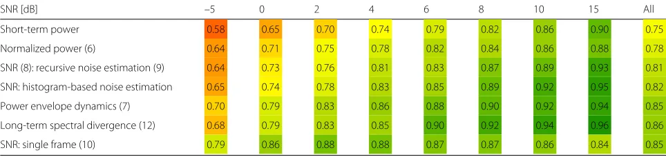
The power and SNR features summarized in this section are now evaluated. We expect that the SNR of the noisy speech signal significantly influences the VAD result. Hence, for this category of features, we focus on the SNR dependency. In Table 1, the performances of some rep-resentative power and SNR features for varying SNR are compared.

Table 1AUC for power and SNR features as a function of SNR. Feature performance is highlighted by colors on a scale from red (low) over yellow (reasonable) to green (good)

SNR [dB] –5 0 2 4 6 8 10 15 All

Short-term power 0.58 0.65 0.70 0.74 0.79 0.82 0.86 0.90 0.75

Normalized power (6) 0.64 0.71 0.75 0.78 0.82 0.84 0.86 0.88 0.78

SNR (8): recursive noise estimation (9) 0.64 0.73 0.76 0.81 0.83 0.87 0.89 0.93 0.81

SNR: histogram-based noise estimation 0.65 0.74 0.78 0.83 0.85 0.89 0.92 0.95 0.82

Power envelope dynamics (7) 0.70 0.79 0.83 0.86 0.88 0.90 0.92 0.94 0.85

Long-term spectral divergence (12) 0.68 0.79 0.83 0.85 0.90 0.92 0.94 0.96 0.86

SNR: single frame (10) 0.79 0.86 0.88 0.88 0.87 0.87 0.86 0.84 0.85

a relatively constant performance. Even the plain short-term power results in a reasonable performance for higher SNRs. However, since no normalization is involved, the overall performance is clearly outperformed by the other approaches.

Normalizing the power based on the maximum and minimum values of the complete utterance (Eq. (6)) improves the results for low SNRs. Since the maximum value is assumed to correspond to speech, this normal-ization is vulnerable against outliers, e.g. noise bursts. In addition, the whole utterance has to be available, which is inapplicable for real-time use cases.

A normalization based on an estimate of the noise power is calculated for the instantaneous SNR (8). For our simulations, we used two different noise power estima-tors. Recursive noise estimation based on the VAD result (9) slightly improves the performance. A similar result is achieved by estimating the noise power based on a histogram.

The next approach tracks the power envelope dynamics (7) to normalize the power. Improvements are achieved by calculating the normalized power for different frequency ranges. This procedure implicitly considers temporal con-text, since the power envelope is tracked slowly over time.

The long-term spectral divergence (LTSD) measure (12) explicitly addresses the temporal context for VAD. Since the maximum value of the power spectrum over mul-tiple frames is employed in the feature, short missed detections can be avoided. This improves the feature’s per-formance consistently. The definition of LTSD includes a look-ahead, so the current decision is influenced by future frames. Especially, onsets are detected more robustly; however, an additional latency in the application has to be tolerated.

The last feature evaluated for this category estimates the SNR based on a single frame (10). A completely different behavior can be observed compared to the features eval-uated before. For the feature, the ratio of the highest and lowest bins of a whitened and sorted power spectrum is

calculated. The whitening thereby can be seen as a simple noise reduction. For low SNRs, the performance there-fore exceeds the results of the other features. On the other hand, even the lowest spectral bins may contain fractions of speech. They are, however, expected to correspond to noise. For higher SNRs, this results in a decreasing performance of the feature.

4.3 Pitch and harmonicity

According to Fant’s source-filter model of human speech production, speech can be modeled by a voiced or unvoiced excitation signal that is spectrally shaped by the vocal tract. In this section, we will discuss features that target at the voiced excitation. Properties of the vocal tract will be revisited later in Section 4.5.

For voiced phonemes, vibration of the vocal cords pro-duce a harmonically rich sound with a distinct pitch between 50 and 250 Hz [25]. All vowels, but some con-sonants as well, exhibit this harmonic structure, which is therefore characteristic for speech. Features that rep-resent the harmonic structure are reliable indicators for speech. However, unvoiced speech portions, such as some fricatives, cannot be expected to be detected using har-monicity or pitch-based features alone [26]. Moreover, music or other harmonic noise components might be misinterpreted as speech.

Voicing properties of speech are employed by sev-eral features [27] with varying complexity. Some simple features only consider variations along time or fre-quency without addressing the harmonic structure. More advanced approaches represent the harmonic structure of voiced speech:

The zero-crossing rate (ZCR) [9] for unvoiced speech is typically higher than that for voiced speech segments. A high value of

ZCR()= L−N+2

n=L

|sign(x(n))−sign(x(n−1))|

therefore can be employed to detect unvoiced phonemes. A combination of the inverse ZCR and the short-term energy

ZRMSE()=

σ2

x()/ZCR() (14)

was proposed in [28] and appeared to be a good measure for the degree of voicing.

The (normalized) auto-correlation function (ACF)

ACF(τ,)=

L−N+1+τ n=L

x(n)·x(n−τ)

norm(τ,) (15)

captures the harmonic structure of speech. Normalization is based on the energy of the signal [27] norm(τ,) =

L−N+1+τ

n=L x2(n)·

_L−N+1

n=L−τ x2(n). The ACF is a fun-damental approach for several pitch-related features for speech detection. For periodic signals, it is maximized for values of τ being integer multiples of the period. This property is employed by features that reflect the maximum ACF peak [27], the periodicity of the ACF [29], or the difference between maximum and minimum values [30].

Some alternative measures similar to ACF were pro-posed. Tucker [11] introduced a periodicity measure that is based on a least squares periodicity estimator. The short-time average magnitude difference function (AMDF) [31] replaces the product operation of the corre-lation by the magnitude of the difference|x(n)−x(n−τ)|. A generalization of the ACF is given by the shift ACF [32] that exploits multiple repetitions of the periodic signal.

The ACF represents the harmonic excitation of the vocal cords. However, it also reflects properties of the vocal tract. To separate both effects, the cepstrum can be employed instead [27]. A log operation is applied to the spectrumxx(ˆ k,)before it is transformed to the cepstral domain using, e.g., the discrete cosine transform (DCT)

cepst(τ,) (16)

The logarithm converts the convolutive mixture in the time domain between excitation signal and vocal tract properties into a sum of two cepstral components. The rapidly fluctuating excitation spectrum thereby is repre-sented by the higher order cepstral bins. Harmonic com-ponents are characterized by a peak in this region. They can be captured using the difference between maximum and minimum value of the cepstrum. Another harmonic feature can be derived by transforming this region of the cepstrum back into the spectral domain [33]. The proper-ties of the vocal tract given by the lower order bins will be discussed in the next section.

The features discussed so far search for periodicity in the time domain1_{. A basic feature in the frequency domain}

is the spectral entropy

normalized spectrum. The entropy reflects the flatness of the spectrum. It is maximized when all spectral values are equal. For speech, some frequencies are excited and domi-nate the spectrum. In this case, the entropy is low, whereas for stationary background noise, high entropy is assumed [27]. Another feature closely related to the entropy is the spectral flatness measure [34]. It is based on the ratio between geometric and arithmetic mean of the spectral values. Both features consider the distribution of spec-tral values. However, they do not explicitly target at the harmonic structure.2

In the frequency domain, the harmonic structure can be described by equally spaced spectral peaks with a dis-tance corresponding to the pitch frequency. The harmonic product spectrum (HPS)

accumulates Rharmonic components corresponding to the potential pitch k˜. The maximum value can be employed to detect periodicity [30].

Normalizing the maximum value based on an estimate of the aperiodic components increases the robustness of the feature as described in [25] and similarly in [35].

4.4 Evaluation of pitch and harmonicity features

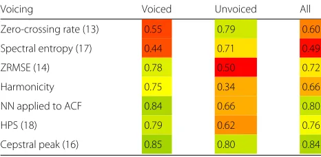
The voicing properties of speech are relevant for the eval-uation of the features discussed in this section. We there-fore analyze the performance on voiced and unvoiced speech portions separately. The results are summarized in Table 2. Our initial analysis showed that noise is a serious problem for these features since the harmonic structure

Table 2AUC for harmonicity features as a function of voicing. A Wiener filter with up to a 6 dB noise suppression was applied as preprocessing. Feature performance is highlighted by colors on a scale from red (low) over yellow (reasonable) to green (good)

Voicing Voiced Unvoiced All

Zero-crossing rate (13) 0.55 0.79 0.60

Spectral entropy (17) 0.44 0.71 0.49

ZRMSE (14) 0.78 0.50 0.72

Harmonicity 0.75 0.34 0.66

NN applied to ACF 0.84 0.66 0.80

HPS (18) 0.79 0.62 0.76

of speech is superimposed by the noise. We therefore apply a Wiener filter with a maximum attenuation of 6 dB to the signal. The noise spectrum is determined using the MMSE-based estimator introduced by Gerkmann and Hendriks [36]. All features discussed in this section are calculated based on this enhanced speech signal.

The ZCR (13) is a feature with low complexity. Our sim-ulation shows that the ZCR for voiced speech behaves similarly compared to the noise-only case. The AUC approaches a value of 0.55, which implies that hardly any separation between voiced speech and noise is possi-ble based on this feature. To distinguish between voiced speech and noise, other features appear to be more appro-priate. On the other hand, unvoiced speech can be reason-ably identified by a high value ZCR.

The spectral entropy (17) shows a behavior similar to the ZCR. The former considers the non-flatness of the spectrum without addressing the harmonic structure. Therefore, it is triggered by unvoiced speech.

The inverse ZCR and the short-term power are com-bined for ZRMSE (14). In contrast to the ZCR, it is capable to detect voiced speech. For voiced speech, the value is high as the power typically is high for voiced speech. On the other hand, the high ZCR for unvoiced speech pre-vents a detector from detecting unvoiced speech. This behavior can be exploited to distinguish between voiced and unvoiced speech.

The next features explicitly focus on the harmonic structure of voiced speech. Typically, pitch is located within a frequency range between 50 and 250 Hz [25]. To determine the degree of harmonicity that corresponds to voiced speech, we therefore restrict all subsequent fea-tures to this frequency range or the corresponding interval of time lags.

Harmonicity is indicated by high peaks max_τ(ACF(τ)) of the normalized ACF (15). Our simulation shows that voiced speech can be identified using this feature. How-ever, noise can also cause peaks in the relevant interval, so the performance is not as good as expected from earlier analyses. To evaluate the general capability of ACF-based features, we apply a neural network to the relevant interval of the ACF. The improved results confirm that better per-formances can be achieved by employing other features than the maximum.

Next, we evaluate the harmonic product spectrum (18) that reflects the harmonic structure of speech in the spectral domain. When calculating max_k˜HPS(k˜), we observe a reasonable performance although no normal-ization is involved.

The cepstral peak max_τ(cepst(τ)) − min_τ(cepst(τ)) (16) shows the best performance of all features consid-ered in this evaluation. For voiced speech, the detection is fine, but even unvoiced speech can be detected using this feature.

4.5 Formant structure

Variable cavities in the human vocal tract allow the speaker to form different phonemes. The resonance (or formant) frequencies are emphasized resulting in a char-acteristic shape of the spectral envelope. Based on this formant structure, specific phonemes can be identified. It is therefore an important feature for speech recognition systems.

The spectral shape of a signal can be described in different ways.

The cepstral coefficients given by Eq. (16) separate the spectral envelope from the excitation. The spectral shape is characterized by the lower order coefficients [37].

Mel frequency cepstral coefficients (MFCCs) rely on a perceptually motivated transformation of the frequency axis. The spectral magnitude values of multiple subbands are accumulated3 _{resulting in a reduced frequency}

res-olution for higher frequencies. Finally, the cepstrum is calculated based on the modified spectrum [38, 39].

Considering the speech signal as the output of an infi-nite impulse response (IIR) filter, the filter coefficients can be determined using linear prediction. The linear predic-tive coding (LPC) coefficients model the spectral shape and can be used for speech detection [10]. An alterna-tive representation of the LPC coefficients is given by the line spectral frequencies (LSFs). LSFs can be interpolated while retaining stability of the corresponding IIR filter. For this reason, it is utilized in the standardized VAD procedure ITU-T G.729 Annex B [22].

To detect speech based on the spectral shape, the mul-tidimensional feature vectors are typically modeled using codebooks. Speech and noise spectra are represented by the different codebook entries. Generally, the codebooks are generated in advance based on a representative train-ing dataset [10]. However, adaptive procedures were also introduced that update the codebook entries based on the recording at hand [39, 40].

4.6 Evaluation of formant structure features

In the following, the features that reflect the formant structure of speech are evaluated. At first, the outputs of the features are multidimensional. Therefore, we classify the results using neural networks. We chose neural net-works in place of codebooks in order to have a common classifier for the multidimensional features from all cat-egories. An evaluation of the performance for different values of the SNR are shown in Table 3.

Table 3AUC for formant features as a function of SNR. Feature performance is highlighted by colors on a scale from red (low) over yellow (reasonable) to green (good)

SNR [dB] –5 0 2 4 6 8 10 15 All

Cepstrum (16) 0.67 0.75 0.80 0.84 0.88 0.90 0.93 0.96 0.85

LPC coefficients 0.59 0.66 0.67 0.70 0.71 0.71 0.73 0.74 0.69

Line spectral frequencies 0.72 0.79 0.82 0.84 0.85 0.87 0.88 0.89 0.83

Mel-filtered spectrum 0.71 0.81 0.86 0.90 0.93 0.95 0.97 0.98 0.90

To evaluate the performance of linear prediction, we used a 10th-order predictor. When applying the neural network directly to the LPC coefficients, we notice that the performance decreases extremely. However, after con-verting the LPC coefficients to line spectral frequencies, a performance similar to that of the cepstrum is achieved. The neural network appears to deal better with LSFs.

An evaluation of the perceptually motivated compres-sion of the spectrum using a mel filterbank is presented in the last row of the table. We applied a neural network to the output of a 20-band mel filterbank. For this category, we achieve the best results.

4.7 Stationarity

The temporal variation of noise is typically much slower than the variation of speech. Under the assumption that noise is a stationary signal, the degree of non-stationarity can be employed for speech detection. Since short-term stationarity is also expected for speech signals, station-arity has to be considered over intervals longer than the typical duration of a phoneme [41]. Unfortunately, non-stationary interferences might trigger speech detectors as well. This suggests applying stationarity-based features primarily in scenarios where non-stationary interferences are unlikely to occur.

Ghosh et al. [41] introduced the long-term signal variability (LTSV) as a measure for non-stationarity. For each frequency bin, a temporal entropy H(k,) = contrast to the spectral entropy given in Eq. (17), the entropy here reflects the temporal flatness for each fre-quency bin over a window of R frames. For stationary signals, the entropy is maximized as the spectrum does not change over time. For the final feature, the entropies of all subbands are fused by calculating the variance over frequency:

Since all entropy values are equal for stationary signals, the feature value approaches zero in this case. When speech is present, non-stationarity occurs in some sub-bands and the variance is higher.

In [42], the procedure was extended to the multi-band LTSV. In contrast to LTSV, the variance is not calculated over all subbands. Instead, multiple variances are deter-mined for different frequency ranges resulting in a multi-dimensional feature vector. This algorithm was reported to deal with non-stationary noise better than the standard LTSV.

The long-term spectral flatness measure (LSFM) was introduced by Ma and Nishihara [43]. For this feature, the entropy is replaced by the ratio of geometric and arithmetic means overRframes.

By calculating the mean over frequency

LSFM()= 1

the subband results are fused. The arithmetic mean gen-erally exceeds the geometric mean. Hence, the feature value is always negative. Speech is indicated by a higher magnitude of the value.

Analogous to the spectral entropy in (17), the features described in this section only consider the distribution of spectral values but do not target at their temporal structure. In the next section, we will therefore focus on modulation features that address the temporal structure of speech. Both stationarity and modulation features will then be evaluated together.

4.8 Modulation

The temporal structure of speech is dominated by a char-acteristic energy modulation peak at about 4 Hz [44]. This frequency corresponds to the typical syllable rate of human speech. Features that target at this property are robust against most interferences; however, a long window is necessary to capture it properly.

Based on the spectrogram that describes the tempo-ral evolution of the spectrum, modulation properties can be determined. Different representations of the spectro-gram were discussed in literature. For example, a sequence of frames of the spectrum xx(ˆ k,) given by Eq. (5) is employed in [45]. For many approaches, a mel filterbank [44] or similar transformations [46] are applied to the spectrum. This results in a perceptually motivated repre-sentation of the spectrogram. Mesgarani et al. [15] even introduced a model of the early-stage auditory system to determine an auditory spectrogram.

each band of a mel-filtered spectrogram, and the cor-responding energy is determined. Based on the overall energy for each band, the energy at 4 Hz is normalized. The average of the normalized values over all bands is employed as a scalar feature for speech detection.

The amplitude modulation spectrogram (AMS) [46] evaluates the modulation for multiple frequencies. For this, a DFT is applied to each band of the spectrogram. To capture the low modulation frequencies around 4 Hz, a long window length of about 1 s was chosen by Bach et al. [47]4. Their implementation considers 29 modu-lation frequencies for 17 frequency bands resulting in a 493-dimensional feature. A more general representation of temporal modulations is given by this feature.

The spectro-temporal modulation (STM) [15] consid-ers modulations along time as well as along frequency. It is motivated by human audio processing in the auditory cortex. In addition to the temporal structure reflected by the AMS, the STM also reveals the harmonic and formant structure of speech [48].

Two-dimensional filters, sometimes called spectro-temporal modulation filters (STMFs), are applied to the spectrogram

r(k,,ω,)= ˆxx(k,) ∗k, STMF(k,;ω,) (22)

where ∗k_, denotes a convolution along time and fre-quency. The STMFs are parametrized by a rate ω [Hz] and a scale parameter [s] that describe the modula-tions along time and frequency. An envelope function, e.g., a Hann window, is applied to limit the size of the two-dimensional FIR filter. An example for STMFs with different parameters is shown in Fig. 2.

Fig. 2STMFs [49] for four different values of_ωand

When the stacked output vectorr()of different filters is directly employed as a feature, the VAD has to deal with a high number of dimensions. In [15], 5 scale filters and 12 rate filters were applied for 128 subbands resulting in a feature vector with 7680 elements.

Different strategies were discussed to reduce the num-ber of dimensions. In [15], a multidimensional PCA was applied. By averaging the magnitude ofr(k,,ω,)over frequency, a feature

E(,ω,)= K−1

k=0

|r(k,,ω,)| (23)

with a reduced number of dimensions was derived by Hsu et al. [45]. They identified max(E(, 1 Hz, 5 ms), E(,−1 Hz, 5 ms))to be a reasonable scalar feature for the detection of speech.

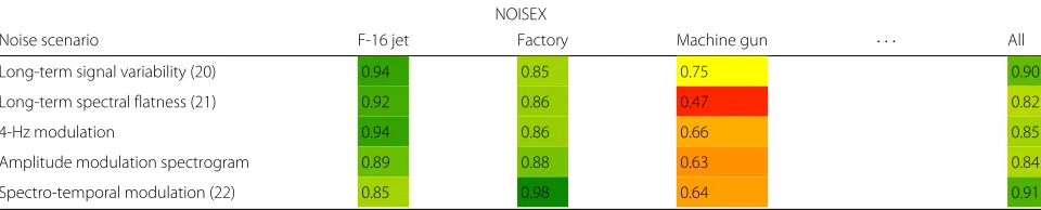
4.9 Evaluation of stationarity and modulation features As discussed, we expect that stationarity features perform best in stationary noise situations. The modulation con-siders the temporal structure of speech and is therefore expected to cope with non-stationary noises. To analyze the robustness against various types of noises, different scenarios from QUT-NOISE and the NOISEX database are taken into account. Our simulation results are sum-marized in Tables 4 and 5. In the table, only some selected scenarios are depicted. Nevertheless, the results over all scenarios are determined based on all noises of each database.

In the first two rows, the evaluation results of the sta-tionarity features, LTSV (20) and LSFM (21), are depicted. For our simulation, both features take into account 30 frames, corresponding to about 0.5 s. As expected, the best performance is achieved for stationary scenarios, such as car noise. The performance decreases for non-stationary scenarios, e.g., the babble noise recorded in a cafe. Obviously, the most challenging scenario is given by the machine gun noise taken from the NOISEX database. The highly non-stationary noise bursts result in a low performance for all features.

In the following, three modulation features are eval-uated. All of these features were calculated based on a mel-filtered spectrogram with 20 bands.

First, the results for the modulation at a frequency of 4 Hz are depicted. A similar performance compared to the stationarity features is noticeable.

Table 4AUC for stationarity and modulation features for some dedicated noise scenarios. The evaluation over all scenarios includes those that are not shown in the table. Feature performance is highlighted by colors on a scale from red (low) over yellow (reasonable) to green (good)

QUT-NOISE

Noise scenario Cafe Kitchen Car (window closed) Pool (reverberant) · · · All

Long-term signal variability (20) 0.78 0.80 0.96 0.95 0.89

Long-term spectral flatness (21) 0.79 0.76 0.94 0.94 0.87

4-Hz modulation 0.79 0.78 0.89 0.93 0.86

Amplitude modulation spectrogram 0.86 0.84 0.94 0.95 0.90

Spectro-temporal modulation (22) 0.95 0.88 0.99 0.99 0.96

The best performance can be observed for the spectro-temporal modulation feature. We employed a feature vec-tor with 771 elements using the Gabor STMFs by Schädler et al. [49]. In almost all scenarios, the STM feature outper-forms the other ones.

4.10 Other features

In literature, one can find many additional approaches, which cannot easily be classified in the categories we described in this article. To present a more complete overview of VAD features, we briefly summarize some of these approaches:

• Teager energy operator (TEO) [50] is based on a non-linear operation on the signal. A multi-band implementation of the feature was discussed [51].

• Higher-order statistics in the LPC residual domain [52] rely on linear prediction as a preprocessing step. Skewness and kurtosis of the residual signal are employed in the feature.

• Modified group delay [53] employs phase information in contrast to the pure magnitude information given by the power spectrum.

• Spectral flux [30, 54] considers local spectral differences between two adjacent frames.

• CASA-based features [55] realize VAD with features that were originally derived in the context of

computational auditory scene analysis (CASA) research.

Statistical model-based approaches comprise the feature and parts of the detector. Since they represent an impor-tant class of VAD algorithms, in the following, we will discuss them in more detail.

4.11 Statistical model-based approaches

The features discussed so far are directly extracted from the data. In the detector, a fixed threshold is applied to the features to make a decision on the presence of speech. Reasonable values of the threshold are usually found heuristically based on histograms. The histograms represent non-parametric estimators of distributions of the features for speech and noise.

The statistical model-based approaches employ the same basic features but extend the decision by prior knowledge of speech. The distributions of features for speech and noise are explicitly modeled by probability density functions (PDFs). Parameters of the PDFs are estimated during runtime. In contrast to the heuristic approaches, a threshold is now applied to the likelihood ratio of the speech and the noise model.

Sohn et al. [12] introduced a frequently cited model-based approach for VAD. They modeled the DFT bins X(k,) by zero-mean complex-Gaussian distributions with different variances for speech and noise. Given

Table 5AUC for stationarity and modulation features for some dedicated noise scenarios. The evaluation over all scenarios includes those that are not shown in the table. Feature performance is highlighted by colors on a scale from red (low) over yellow (reasonable) to green (good)

NOISEX

Noise scenario F-16 jet Factory Machine gun · · · All

Long-term signal variability (20) 0.94 0.85 0.75 0.90

Long-term spectral flatness (21) 0.92 0.86 0.47 0.82

4-Hz modulation 0.94 0.86 0.66 0.85

Amplitude modulation spectrogram 0.89 0.88 0.63 0.84

the hypotheses defined in (2), the resulting likelihood ratio

(k,)= p(X(k,)|H1) p(X(k,)|H0)

(24)

= 1

1+ξ(k,)exp

_{γ (}

k,)·ξ(k,) 1+ξ(k,)

(25)

for each frequency bin depends on the a priori SNRξ(k,) and the a posteriori SNRγ (k,). Both parameters are esti-mated based on the observed data using the estimator introduced by Ephraim and Malah [56]. Since statistical independence between frequency bins is assumed, the final likelihood ratio is derived as the geometric mean over frequency log()= _K1_kK₌−₀1log(k,).

Other distributions were investigated that model speech more accurately than Gaussian PDFs. Chang et al. [57] chose a complex Laplacian model that was replaced in [58] by a generalized gamma distribution. A comparison between different models was presented in [13].

The likelihood ratio in (24) is calculated based on a single frame. Especially weak speech tails are difficult to detect given this limited amount of information. In sev-eral publications, model-based VADs were discussed that incorporate contextual information from multiple frames. Already Sohn et al. [12] introduced a hangover scheme that considers the dependency between successive frames. For this, speech and speech pause are modeled by two states of a hidden Markov model (HMM). Fixed probabil-ities are assigned to both state transitions. The forward procedure is applied, resulting in a temporally smoothed likelihood ratio.

Ramírez et al. [59] formulated a multiple-observation likelihood ratio test (MO-LRT) for VAD. In addition to the assumption of statistical independence between fre-quency bins, 2R+1 successive frames are also assumed to be independent. This results in a likelihood ratio MO-LRT() = Rr=−R(+r). Ramírez et al. reported an improved reliability of VAD, even though it was men-tioned that the assumption of independence does not hold in most cases.

Shin et al. [60] considered the inter-frame correlation by conditioning the PDF based on the previous frame. They derived an approach that applies two different thresh-olds to the likelihood ratio depending on the previous VAD result. Later, in [61] the approach was refined by considering the two preceding frames.

5 Inter-category evaluation

In the preceding sections, we separately discussed features that reflect different properties of speech. The evalua-tions of dedicated features revealed that their VAD per-formance varies even when the same speech property is employed. We measured the performance in terms of area under ROC curve (AUC) values.

Here, we change our perspective from specific features towards the practicability of feature classes for applica-tions. In addition to the average performance given by the AUC, the temporal behavior of features will be rele-vant for this consideration. We will quantify this temporal behavior using the measures summarized in Section 2.1. The results are interpreted with respect to the temporal context and look-ahead employed by the features.

Temporal context and look-ahead are in general bene-ficial for detection performance. Speech onsets are more accurately captured due to the look-ahead. The tempo-ral context allows for detection of weak phonemes by employing information from adjacent frames.

However, look-ahead is only applicable for some use cases. In an implementation, the acausal look-ahead is resolved by delaying other parts of the application. This delay between input and output signal is unac-ceptable when both signals are simultaneously available to a listener. Delays have to be avoided, e.g., in hear-ing aids, where the amplified output signal superimposes with the direct sound. Additionally, current values, e.g., a spectrum, have to be buffered for later usage. The increased memory consumption is another drawback of look-ahead.

To employ temporal context in VAD features, some information, e.g., multiple frames of the spectrum, have to be stored. Again, the memory consumption increases, which is crucial for applications that deal with limited resources.

In the following, we will analyze the temporal behavior of different features for each category.

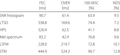
The fine-grained measure of the dynamic behavior allows for an intuitive interpretation of the feature’s per-formance. To determine the detection rate, detection results for frames close to reference speech onsets and offsets are averaged over multiple utterances. Plots of the dynamic behavior are shown in Figs. 3 and 4. The cor-responding values of FEC, OVER, MSC, and NDS are summarized in Table 6. For FEC, the average time-lag between onset and the first following detection is calcu-lated. Analogously, the average time-lag between offset and the following stop of detection is considered for OVER. To achieve positive values for FEC and OVER, feature look-aheads are compensated before evaluation. MSC and NDS are expressed by the detection rate in the remaining intervals that are not already covered by FEC and OVER as illustrated in Fig. 1. For all anal-yses described in this section, we fix the false alarm rate to Pfa(η10%) = 0.1 by adjusting the threshold η10%

accordingly.

Fig. 3Dynamic behavior (a,b) and ROC curve (c) for two different features. The LTSD feature considers some temporal context whereas the SNR feature relies on a single frame. The ROC curve plots the average detection rate during speech intervalsPd(η)vs. the average false-alarm rate during noise-only intervalsPfa(η)for varying values of the thresholdη. The dynamic behavior reflects the time dependency of detections relative to speech onsets and offsets for a fixed thresholdη10%chosen such thatPfa(η10%)=0.1

feature is calculated based on 2R+1 frames. A look-ahead ofRframes allows the LTSD feature to even consider some future data.

In Fig. 3, the dynamic behavior as well as the ROC curve are depicted for both features. The ROC curve for LTSD reveals an improved performance compared to the SNR feature. The curve for LTSD is located closer to the opti-mal point that is given by the upper left corner of the plot (Pd = 1,Pfa = 0). The dynamic behavior shows a

slightly decreasing detection rate over time for both fea-tures. Again, the detection rate of LTSD always exceeds the SNR feature.

The temporal context and the look-ahead of LTSD are reflected in the plot. Using LTSD, speech is already detected before the reference indicates the presence of speech. On the other hand, the feature retains high val-ues for a short period of time after reference offsets. The inert reaction of LTSD to speech onsets and offsets is quantified by higher values of FEC and OVER in Table 6. Even though slightly different intervals are considered for

Fig. 4Dynamic behavior for features that represent harmonicity (HPS), formant structure (Mel spectrum), stationarity (LSFM), or modulation (STM) of speech

100-MSC andPd(η10%)as well as NDS andPfa(η10%), the

results exhibit the same tendency.

The fine-grained measure of the dynamic behavior apparently provides more information about the feature compared to FEC, OVER, MSC, and NDS. For the fol-lowing discussions, we therefore focus on the fine-grained measure.

The dynamic behavior of representative features from other categories is depicted in Fig. 4. Obviously, the fea-tures for harmonicity (HPS) and formant structure (Mel spectrum) indicate speech only in the reference speech interval. Since both properties are calculated instanta-neously without temporal context, speech onsets and offsets are precisely localized. No distinction is made between voiced and unvoiced speech portions for this analysis. The HPS feature is therefore outperformed by all other features considered here. Nevertheless, harmonicity features are typically less complex and provide reasonable results for voiced speech as discussed in Section 4.3.

The formant structure, represented by the Mel spec-trum, improves the performance compared to har-monicity. However, features that employ the formant structure are typically multidimensional and require a

Table 6Time-selective evaluation measures applied to different features from all categories

FEC OVER 100-MSC NDS

[ms] [ms] [%] [%]

SNR histogram 90.7 61.4 63.9 9.5

LTSD 338.8 169.6 74.4 7.2

HPS 320.4 62.5 41.1 8.8

Mel spectrum 83.2 42.9 76.8 9.6

LSFM 228.0 219.7 72.8 10.1

more complex decision scheme, e.g., based on codebooks or neural networks.

The LSFM feature exemplifies stationarity properties of speech. No look-ahead is introduced, the VAD therefore starts to detect speech after the reference onset. The tem-poral context of 0.5 s is reflected by the plot of the dynamic behavior.

Modulation properties of speech are considered by the STM feature. The feature outperforms all other features in this analysis. Since a long temporal context and look-ahead are involved, the feature indicates speech for some time before the reference onset and after the offset. Cal-culation of the feature is quite complex. On the one hand, several frames of the spectrum have to be stored which increases the memory consumption. On the other hand, much CPU is required to convolve the spectrogram with different filters and fuse the individual results to a final VAD.

6 Conclusions

In this article, we have summarized and analyzed several features for voice activity detection. Under the objec-tive to categorize features by speech properties that are employed, we have given an overview of established approaches. Our analyses showed that the performances of features vary, even when the same speech property was considered. We have identified the temporal context as one important aspect for improved performance.

A long temporal context and look-ahead are benefi-cial for speech detection. However, both can be utilized only in some applications. On the one hand, the mem-ory and CPU consumption typically increase for a longer context. This is critical for applications that have to deal with limited resources. On the other hand, delays have to be inserted for the implementation of a look-ahead. This can only be afforded for applications where an immediate availability of the result is less important.

We have compared the temporal behavior of represen-tative features from all categories. It became obvious that power, harmonicity, and formant structure of speech can be captured without exploiting temporal context informa-tion. In contrast, stationarity and modulation properties of speech have to be extracted based on a longer context.

Throughout the article, we have focused on discussing separate features. However, combinations of features from different categories seem to be promising. Independent properties of speech should be employed together, result-ing in an improved performance.

Endnotes

1_{In case of the cepstrum, it is the frequency domain.}

2_{In fact, reordering of the spectral bins does not}

influence the features, which implies that they are triggered by any non-flat spectrum.

3_{According to some definitions (e.g., [38]), a logarithm}

is calculated before accumulating.

4_{In an earlier approach [46], a short window length was}

chosen, too short to resolve the 4-Hz modulation. However, it was stated that even short segments can be sufficient to identify speech.

Competing interests

The authors declare that they have no competing interests.

Received: 1 July 2015 Accepted: 26 October 2015

References

1. M Espi, S Miyabe, T Nishimoto, N Ono, S Sagayama, inProc. of Spoken language technology workshop (SLT). Analysis on speech characteristics for robust voice activity detection (IEEE, Berkeley, California, USA, 2010) 2. M Van Segbroeck, A Tsiartas, SS Narayanan, inProc. of INTERSPEECH. A

robust frontend for VAD: exploiting contextual, discriminative and spectral cues of human voice (ISCA, Lyon, France, 2013)

3. DK Freeman, CB Southcott, I Boyd, inProc. of IEE Colloquium on Digitized Speech Communication via Mobile Radio. A voice activity detector for the Pan-European digital cellular mobile telephone service (IEEE, London, United Kingdom, 1988)

4. S Graf, T Herbig, M Buck, G Schmidt, inProc. of ITG conference on speech communication. Improved performance measures for voice activity detection (IEEE, Erlangen, Germany, 2014)

5. DB Dean, S Sridharan, RJ Vogt, MW Mason, inProc. of INTERSPEECH. The QUT-NOISE-TIMIT corpus for the evaluation of voice activity detection algorithms (ISCA, Makuhari, Japan, 2010)

6. A Varga, HJM Steeneken, Assessment for automatic speech recognition: II, NOISEX-92: a database and an experiment to study the effect of additive noise on speech recognition systems. Speech Commun.12(3), 247–251 (1993)

7. JS Garofolo, LF Lamel, WM Fisher, JG Fiscus, DS Pallet, NL Dahlgren, DARPA TIMIT acoustic-phonetic continuous speech corpus CD-ROM. National Institute of Standards and Technology (1993)

8. J-C Junqua, The influence of acoustics on speech production: a noise-induced stress phenomenon known as the Lombard reflex. Speech Commun.20(1), 13–22 (1996)

9. LR Rabiner, MR Sambur, An algorithm for determining the endpoints of isolated utterances. Bell Syst. Tech. J.54(2), 297–315 (1975)

10. LR Rabiner, MR Sambur, Application of an LPC distance measure to the voiced-unvoiced-silence detection problem. IEEE Trans. Acoust. Speech Signal Process.25(4), 338–343 (1977)

11. R Tucker, Voice activity detection using a periodicity measure. IEEE Proc. Commun. Speech Vis.139(4), 377–380 (1992)

12. J Sohn, NS Kim, W Sung, A statistical model-based voice activity detection. IEEE Signal Process. Lett.6(1), 1–3 (1999)

13. J-H Chang, NS Kim, SK Mitra, Voice activity detection based on multiple statistical models. IEEE Trans. Signal Process.54(6), 1965–1976 (2006) 14. J Ramírez, JC Segura, C Benítez, Á de la Torre, A Rubio, Efficient voice activity detection algorithms using long-term speech information. Speech Commun.42, 271–287 (2004)

15. N Mesgarani, M Slaney, SA Shamma, Discrimination of speech from nonspeech based on multiscale spectro-temporal modulations. IEEE Trans. Audio, Speech Lang. Process.14(3), 920–930 (2006)

16. J Anemüller, D Schmidt, J-H Bach, inProc. of INTERSPEECH. Detection of speech embedded in real acoustic background based on amplitude modulation spectrogram features (ISCA, Brisbane, Australia, 2008) 17. M Marzinzik, B Kollmeier, Speech pause detection for noise spectrum

estimation by tracking power envelope dynamics. IEEE Trans. Speech Audio Process.10(2), 109–118 (2002)

18. LF Lamel, LR Rabiner, AE Rosenberg, JG Wilpon, An improved endpoint detector for isolated word recognition. IEEE Trans. Acoust. Speech Signal Process.29(4), 777–785 (1981)

19. S Van Gerven, F Xie, inProc. of EUROSPEECH. A comparative study of speech detection methods (ISCA, Rhodos, Greece, 1997)

21. J Ramírez, JC Segura, C Benítez, A de La Torre, A Rubio, inProc. of ICASSP. A new voice activity detector using subband order-statistics filters for robust speech recognition (IEEE, Montreal, Canada, 2004) 22. ITU, ITU-T Recommendation G.729 Annex B A silence compression

scheme for G.729 optimized for terminals conforming to Recommendation V.70 (1996)

23. ETSI, ETSI EN 301 708 Voice activity detector (VAD) for adaptive multi-rate (AMR) speech traffic channels (1998)

24. ETSI, ETSI ES 202 050 Advanced front-end feature extraction algorithm (2007)

25. DJ Nelson, J Pencak, inProc. of SPIE’s 1995 International Symposium on Optical Science, Engineering, and Instrumentation. Pitch-based methods for speech detection and automatic frequency recovery (International Society for Optics and Photonics, San-Diego, California, USA, 1995) 26. G Hu, D Wang, Segregation of unvoiced speech from nonspeech

interference. J. Acoust. Soc. Am.124(2), 1306–1319 (2008)

27. T Kristjansson, S Deligne, P Olsen, inProc. of INTERSPEECH. Voicing features for robust speech detection (ISCA, Lisbon, Portugal, 2005)

28. C Shahnaz, W-P Zhu, MO Ahmad, inProc. of ISCAS. A multifeature voiced/unvoiced decision algorithm for noisy speech (IEEE, Kos, Greece, 2006)

29. H Ghaemmaghami, BJ Baker, RJ Vogt, S Sridharan, inProc. of INTERSPEECH. Noise robust voice activity detection using features extracted from the time-domain autocorrelation function (ISCA, Makuhari, Japan, 2010) 30. SO Sadjadi, JHL Hansen, Unsupervised speech activity detection using

voicing measures and perceptual spectral flux. IEEE Signal Process. Lett. 20(3), 197–200 (2013)

31. M Orlandi, A Santarelli, D Falavigna, inProc. of INTERSPEECH. Maximum likelihood endpoint detection with time-domain features (ISCA, Geneva, Switzerland, 2003)

32. F Kurth, A Cornaggia-Urrigshardt, inProc. of ITG Conference on Speech Communication. Detection of audio events with repetitive structure using generalized autocorrelations (IEEE, Erlangen, Germany, 2014)

33. T Fukuda, O Ichikawa, M Nishimura, inProc. of ICASSP. Improved voice activity detection using static harmonic features (IEEE, Dallas, Texas, USA, 2010)

34. N Madhu, Note on measures for spectral flatness. Electron. Lett.45(23), 1195–1196 (2009)

35. K Ishizuka, T Nakatani, inProc. of SAPA. Study of noise robust voice activity detection based on periodic component to aperiodic component ratio (ISCA, Pittsburgh, Pennsylvania, USA, 2006)

36. T Gerkmann, RC Hendriks, Unbiased MMSE-based noise power estimation with low complexity and low tracking delay. IEEE Trans. Audio, Speech, Lang. Process.20(4), 1383–1393 (2012)

37. JA Haigh, JS Mason, inProc. of EUROSPEECH. A voice activity detector based on cepstral analysis (ISCA, Berlin, Germany, 1993)

38. JD Hoyt, H Wechsler, inProc. of ICASSP. Detection of human speech in structured noise (IEEE, Adelaide, Australia, 1994)

39. T Kinnunen, P Rajan, inProc. of ICASSP. A practical, self-adaptive voice activity detector for speaker verification with noisy telephone and microphone data (IEEE, Vancouver, Canada, 2013), pp. 7229–7233 40. F Heese, M Niermann, P Vary, inProc. of ICASSP. Speech-codebook based

soft voice activity detection (IEEE, Brisbane, Australia, 2015)

41. PK Ghosh, A Tsiartas, S Narayanan, Robust voice activity detection using long-term signal variability. IEEE Trans. Audio, Speech, Lang. Process. 19(3), 600–613 (2011)

42. A Tsiartas, T Chaspari, N Katsamanis, P Ghosh, M Li, M Van Segbroeck, A Potamianos, SS Narayanan, inProc. of INTERSPEECH. Multi-band long-term signal variability features for robust voice activity detection (ISCA, Lyon, France, 2013)

43. Y Ma, A Nishihara, Efficient voice activity detection algorithm using long-term spectral flatness measure. EURASIP J. Audio, Speech, Music Process.2013(1), 1–18 (2013)

44. E Scheirer, M Slaney, inProc. of ICASSP. Construction and evaluation of a robust multifeature speech/music discriminator (IEEE, Munich, Germany, 1997)

45. C-C Hsu, T-E Lin, J-H Chen, T-S Chi, inProc. of ICASSP. Voice activity detection based on frequency modulation of harmonics (IEEE, Vancouver, Canada, 2013)

46. J Tchorz, B Kollmeier, inProc. of EUROSPEECH. Speech detection and SNR prediction basing on amplitude modulation pattern recognition (ISCA, Budapest, Hungary, 1999)

47. J-H Bach, B Kollmeier, J Anemüller, inProc. of ICASSP. Modulation-based detection of speech in real background noise: generalization to novel background classes (IEEE, Dallas, Texas, USA, 2010)

48. T Ezzat, J Bouvrie, T Poggio, inProc. of INTERSPEECH. Spectro-temporal analysis of speech using 2-D Gabor filters (ISCA, Antwerp, Belgium, 2007) 49. MR Schädler, BT Meyer, B Kollmeier, Spectro-temporal modulation

subspace-spanning filter bank features for robust automatic speech recognition. J. Acoust. Soc. Am.131, 4134 (2012)

50. GS Ying, CD Mitchell, LH Jamieson, inProc. of ICASSP. Endpoint detection of isolated utterances based on a modified Teager energy measurement (IEEE, Minneapolis, Minnesota, USA, 1993)

51. G Evangelopoulos, P Maragos, Multiband modulation energy tracking for noisy speech detection. IEEE Trans. Audio, Speech Lang. Process.14(6), 2024–2038 (2006)

52. E Nemer, R Goubran, S Mahmoud, Robust voice activity detection using higher-order statistics in the LPC residual domain. IEEE Trans. Speech Audio Process.9(3), 217–231 (2001)

53. RM Hegde, HA Murthy, VR Gadde, inProc. of INTERSPEECH. The modified group delay feature: a new spectral representation of speech (ISCA, Jeju Island, Korea, 2004)

54. N Cho, E-K Kim, Enhanced voice activity detection using acoustic event detection and classification. IEEE Trans. Consum. Electron.57(1), 196–202 (2011)

55. X-L Zhang, D Wang, inProc. of INTERSPEECH. Boosted deep neural networks and multi-resolution Cochleagram features for voice activity detection (ISCA, Singapore, 2014)

56. Y Ephraim, D Malah, Speech enhancement using a minimum-mean square error short-time spectral amplitude estimator. IEEE Trans. Acoust. Speech Signal Process.32(6), 1109–1121 (1984)

57. J-H Chang, JW Shin, NS Kim, inProc. of INTERSPEECH. Likelihood ratio test with complex Laplacian model for voice activity detection (ISCA, Geneva, Switzerland, 2003)

58. JW Shin, J-H Chang, HS Yun, NS Kim, inProc. of ICASSP. Voice activity detection based on generalized gamma distribution (IEEE, Philadelphia, Pennsylvania, USA, 2005)

59. J Ramírez, JC Segura, C Benítez, L García, A Rubio, Statistical voice activity detection using a multiple observation likelihood ratio test. IEEE Signal Process. Lett.12(10), 689–692 (2005)

60. J-W Shin, HJ Kwon, SH Jin, NS Kim, Voice activity detection based on conditional MAP criterion. IEEE Signal Process. Lett.15, 257–260 (2008) 61. S-K Kim, J-H Choi, S-I Kang, J-H Song, J-H Chang, inProc. of INTERSPEECH.

Toward detecting voice activity employing soft decision in second-order conditional MAP (ISCA, Makuhari, Japan, 2010)

Submit your manuscript to a

journal and benefi t from:

7Convenient online submission

7Rigorous peer review

7Immediate publication on acceptance

7Open access: articles freely available online

7High visibility within the fi eld

7Retaining the copyright to your article