Matched, mismatched, and robust scatter matrix estimation and hypothesis testing in complex t distributed data

R E S E A R C H

Open Access

Matched, mismatched, and robust scatter

matrix estimation and hypothesis testing

in complex

t

-distributed data

Stefano Fortunati

, Fulvio Gini

and Maria S. Greco

Abstract

Scatter matrix estimation and hypothesis testing are fundamental inference problems in a wide variety of signal processing applications. In this paper, we investigate and compare the matched, mismatched, and robust approaches to solve these problems in the context of the complex elliptically symmetric (CES) distributions. The matched approach is when the estimation and detection algorithms are tailored on the correct data distribution, whereas the mismatched approach refers to the case when the scatter matrix estimator and the decision rule are derived under a model assumption that is not correct. The robust approach aims at providing good estimation and detection performance, even if suboptimal, over a large set of possible data models, irrespective of the actual data distribution. Specifically, due to its central importance in both the statistical and engineering applications, we assume for the input data a complext-distribution. We analyze scatter matrix estimators derived under the three different approaches and compare their mean square error (MSE) with the constrained Cramér-Rao bound (CCRB) and the constrained misspecified Cramér-Rao bound (CMCRB). In addition, the detection performance and false alarm rate (FAR) of the various detection algorithms are compared with that of the clairvoyant optimum detector.

Keywords:Covariance matrix estimation, Complex elliptically symmetric distribution, Detection problem, Constrained Cramér-Rao bound, Misspecified Cramér-Rao bound

1 Introduction

This paper deals with two common inference problems in radar signal processing, namely the estimation of the disturbance covariance matrix and the adaptive detec-tion of a radar target. In addidetec-tion to the radar detecdetec-tion, the covariance matrix estimation is a fundamental pre-requisite for a lot of applications in many different areas: the direction of arrival (DOA) estimation in array pro-cessing [1], the principal component analysis (PCA) [2], and the portfolio optimization in finance [3], just to name a few. We put the covariance estimation and the adaptive detection problems in the more general context of the scatter matrix estimation and hypothesis testing in the complex elliptically symmetric (CES) distribution family. CES distributions constitute a wide class of distributions that includes the complex Gaussian,

generalized Gaussian, the K-distribution, complex t-dis-tribution and all the compound Gaussian dist-dis-tributions as special cases. Due to their flexibility and their capabil-ity to model a plethora of different data behavior, they are widely applied in many areas, such as radar, sonar, and communications [4, 5]. A CES distribution is com-pletely characterized by the mean valueγ, the scatter (or shape) matrix Σ, and the density generator g. Given a particular CES distribution, its density generator could depends on some extra parameters, (e.g., shape and scale parameters for a complex t-distribution) that are in general unknown and need to be estimated from the data along withγandΣ.

Specifically, because of its generality, several aspects should be taken into account when making inference on the CES class. The first aspect concerns the existence, convergence, and computational complexity of optimal algorithms tailored (matched) to a particular CES distri-bution at hand. Think for example of the problem of the joint estimation of the mean value, of the scatter matrix, * Correspondence:[email protected]

1_{Dipartimento di Ingegneria dell’Informazione, University of Pisa, Via G.} Caruso 16, Pisa 56122, Italy

2

CNIT RaSS (Radar and Surveillance System) National Laboratory, Pisa, Italy

and of the extra parameters that characterize the density generator. As pointed out in, e.g., [6, 7], a joint maximum likelihood (ML) estimation of all these unknown quan-tities would encounter computational difficulties and con-vergence (or even existence) issues. To overcome this problem, one has to rely on suboptimal, computationally inexpensive and easy to implement estimators [8]. A dif-ferent alternative could be to assume a simpler model, e.g., a Gaussian distribution, for the data behavior that al-lows one for an easy derivation of optimal (but generally mismatched) estimators or detection rules [9]. This consideration leads directly to another issue, namely the robustness to misspecification. In particular, it would be of interest to know whether the inference methods based on an assumed CES distribution can achieve“good” perform-ance even if the data follow a different and, in general, more involved CES model. Finally, as direct consequence of the previous considerations, this analysis culminates in the possibility to derive and implement robust infer-ence algorithms with good performance over the whole class of CES distributions, even if not optimal under any nominal model.

Following the line of the previous discussion, in this paper, we investigate and compare the matched, mis-matched, and robust approaches for inference methods in complex t-distributed data. We focus on the multi-variate complex t-distribution, since it has long been recognized by several authors from both the statistical (see, e.g., [6] and the references therein) and the signal processing communities (see, e.g., [10–13]) as a suitable and flexible model able to describe the heavy-tailed behavior of the measurements in many practical applica-tions (e.g., radar detection).

The paper is organized in two parts. In the first part, we investigate the scatter matrix estimation problem. The second part deals with adaptive detection algo-rithms. In particular, in the first part, we investigate the performance loss in the scatter matrix estimation when the unknown extra parameters of the t-distribution are replaced with low computational complexity estimates obtained via the method of moments (MoM). This rep-resents thematched case. The mean square error (MSE) of the “matched” estimators is compared with the con-strained Cramér-Rao bound (CCRB). Then, we address the mismatched case where, following the approach discussed in our recent work [14], the performance of the mismatched ML (MML) scatter matrix estimator derived under Gaussian assumption is evaluated and its MSE compared with the constrained misspecified Cramér-Rao bound (CMRB) [15]. Finally, the min-max robust (among the whole CES class) constrained Tyler (C-Tyler) estimator [16] is introduced and its performance compared with the CCRB and the other previously derived estimators.

The second part of the paper focuses on the detection performance of three detection algorithms: the linear threshold detector(LTD) [12], i.e., thematchedgeneralized likelihood ratio test (GLRT)detectorfor complex t-distrib-uted data; Kelly’s detector [17], i.e., the GLRT detector derived under the misspecified Gaussian distribution; and the adaptive normalized matched filter (ANMF), that represents the robust detector among the CES class. The ANMF has been derived and analyzed by many authors under different names (see, e.g., [4, 18–23]). The three detectors are compared in terms of (i) constant false alarm rate (CFAR) property with respect to (w.r.t.) the scatter matrix and the extra parameters estimation and (ii) receiver operating characteristic (ROC) curves.

The remainder of the paper is organized as follows. In Section 2, a brief review of the main properties of the CES distribution class and of the complex t-distribution is provided. In Section 3, the scatter matrix estimation problem is introduced and the application of the matched, mismatched, and robust approaches extensively analyzed. In Section 4, the hypothesis testing problem in complex t-distributed data is investigated. Section 5 collects the simulation results, while Section 6 summarizes our conclusions.

2 The CES distribution class, the compound-Gaussian subclass, and the complext-distribution

The aim of this section is to provide a brief overview of the CES distribution class and makes no claim to complete-ness. For more comprehensive and detailed discussions, we refer the readers to the excellent works [4] and [5].

A complex N-dimensional random vector xm is CES distributed, in shorthand notationxm~CEN(γ,Σ,g), if its probability density function (pdf ) is of the form

pXð Þ ¼xm cN;gj jΣ−1g ðxm−γÞHΣ−1ðxm−γÞ

; ð1Þ

where g is the density generator, cN,g is a normalizing

constant, γ≜E{xm}, and Σ is the normalized (or shape)

covariance matrix, also calledscatter matrix. Due to the well-known ambiguity between the scatter matrix and the density generator of any CES distribution, a con-straint on the scatter matrix needs to be imposed. In the rest of the paper, we choose to impose the following constraint: tr(Σ) =N. As a consequence, if M≜E{(xm

−γ)(xm−γ)H} is the covariance matrix of the random

vectorxm, then Σ=N/tr(Μ)⋅M. For some CES

distribu-tions, the un-normalized covariance matrix M does not exist, but the scatter matrix Σ is still well-defined. This is the case, for example, for all the CES distributions that do not have finite second-order moments (e.g., the Cauchy distribution) [5]. Based upon the stochastic representation theorem [5], any xm~CEN(γ,Σ,g) with

xm=dγ+RPu, where the non-negative random

vari-able (r.v.) R≜pffiffiffiffiQ, the so-called modular variate, is a real, non-negative random variable, u~U(ℂSk) is a k -dimensional random vector uniformly distributed on the unit hyper-sphere ℂSk with k−1 topological di-mensions such that uHu= 1, R andu are independent, and Σ=PPH is a factorization of Σ, where P is a Nxk matrix and rank(P) =k. It is easy to show that the random vector u is strictly related to a complex nor-mal distribution CN(0,I), where I defines the identity matrix. In fact, if w~CN(0,I), then u=dw/‖w‖ [5].

Using this property, the stochastic decomposition can be recast as xm¼ _dγþRPu¼ _dγþ R= ffiffiffiffiffiffiffiQw

p

ð ÞPw

where Qw≜‖w‖

2

~ Gam(N, 1). Moreover, Qw is

inde-pendent of w, and E{Qw} =N, and E Q2w ¼N Nð þ1Þ

[5]. In the following, we assume that Σ is real and full-rank, i.e., rank(P) = rank(Σ) =N. An important re-mark is in order: for CES distributions, the term σ2≜ E{Q}/N can be interpreted as the statistical power of the random vector xm, i.e., the covariance matrix M,

and the scatter matrix Σ are related by M=σ2Σ. An important subclass of the CES distributions is the compound-Gaussian (CG) distributions [24]. In particular, a CG-distributed random vector xm~ CGN(γ,Σ,pτ) admits the following stochastic

represen-tation xm ¼ dγþ ffiffiffi

τ p

Pw¼_dpffiffiffiffiffiffiffiffiffiffiτ⋅Q_wPu, where, as be-fore, w~CN(0,I), u~U(ℂSN), and Qw~ Gam(N, 1). Usually, the positive real random variable τ is called the texture and the complex Gaussian random vector

n=dPw is called the speckle. It can be noted that a CES-distributed random vector belongs to the sub-class of the CG-distributed random vector if and only if the square of its modular variate R2 can be written as a random scaled gamma distribution, i.e., R2=τ⋅Qw and thenR2|τ~ Gam(N,τ) [5].

At this point, we can introduce the complex t-distribu-tion. A complex N-dimensional zero-mean (γ= 0) ran-dom vectorxmis complext-distributed if its pdf can be expressed as

p_Xðxm;Σ;λ;ηÞ≜

1

πN_{j j}Σ

ΓðNþλÞ Γ λð Þ λη

λ _λ

ηþxHmΣ−1xm −ðNþλÞ

;

ð2Þ

where λ and η are the shape and scale parameters, re-spectively. It is easy to show that the pdf in Eq. (2) is of the form given in Eq. (1) where the density generator can be expressed as g(t) = (λ/η+t)−(N+λ)[5]. Moreover, it can be also shown that it admits a CG representation [24]. The complex t-distribution has tails heavier than the normal one for everyλ∈(0,∞), while the limiting case λ→∞ yields the complex normal distribution. More-over, the statistical power is a function of λ and η as follows [12,14]:

σ2_¼E

pfQΣg=N ¼λ=η λð −1Þ: ð3Þ

Before passing to discuss the scatter matrix estima-tion problem in complex t-distributed data, few re-marks are needed. In the rest of the paper, we always assume that:

i) The dataset x¼f gxm Mm¼1 is composed of M independent and identically distributed (IID) N-dimensional, zero-mean, complex t-distributed random vectors.

ii) The scatter matrixΣis arealandfull rankmatrix.

It must be underlined that the second assumption is quite strong and not always verified in radar/sonar ap-plications. It is well-known in fact that, if the power spectral density (PSD) of the disturbance is not sym-metric around a central frequency, the autocorrelation function of the complex envelope of the data is com-plex valued and consequently also the scatter matrix (see, e.g., [25]). However, working with complex matri-ces would require the use of more sophisticated math-ematical tools, i.e., the so-called Wirtinger calculus [26], but this general approach falls outside the scope of the paper. The case of complex scatter matrix will be considered in future works.

3 Scatter matrix estimation

This section deals with the scatter matrix estimation from a set of IID complex t-distributed data. As discussed in the previous section, we investigate three different ap-proaches: the matched, the mismatched, and the robust cases. We also provide the relative performance bounds, i.e., the CCRB and the CMCRB.

3.1 The matched case for complext-distributed data

In this section, we discuss and derive two matched estimators of the scatter matrix Σ and of the extra parameters λ and η by assuming to know perfectly the correct data model, i.e., the complex t-distribu-tion. Building upon previous results, we investigate the performance of the following two estimators: (1) the constrained maximum likelihood (CML) estimator ofΣwhich uses the method of moments (MoM) estimates of λ and η and (2) a recursive (suboptimal) estimator of Σ, λ, and η.

^

As we can see, Eq. (4) involves the unknown shape and scale parameter of the t-distribution. To estimate them, we use the low computational complexity (but suboptimal) MoM estimators. The MoM method con-sists of equating the experimental moments with the corresponding theoretical ones in order to obtain an estimate of the unknown parameters of interest. In par-ticular, given a random variablerwhose pdf depends on some unknown parameters, one needs to firstly evaluate analytically the moments mk≜E{rk}, i.e., the expected values of powers of the random variable under consider-ation, and, secondly, equate the obtained expressions (that will depend on the unknown parameters) with the corresponding sample estimates of the moments, i.e.,

^

the random variable r.

In the problem at hand, we need to estimate the shape and scale parameters,λandη, of the complex t-distribu-tion. In order to do this, we may apply the MoM method by considering the moments of the amplitude of each entry of the data vector xm, i.e., rn≜|[xm]n|, n= 1,…,N. To evaluate the moments of the amplitude rn, we can exploit the decomposition given in Theorem 5 of [5] and the fact that the t-distribution is a CG distribution. In particular, we have that the amplitude

rn≜xm;n ¼R½Pumn¼

is distributed according to [5] as

p_rnð Þ ¼r 2ηr 1þη λr2 −ðλþ1Þ

u rð Þ; ð6Þ

where u(⋅) is the unit step function. It is easy to verify through direct calculation on the pdf in (6) that the mo-ments of orderkofrnare given by

Finally, by applying the classical MoM approach using the fourth-order and the second-order moments of rn, the parametersλandηcan be estimated as follows [28]:

^

are the sample estimates of the moments. Due to exist-ence issues of the fourth-order moment, we constrain the estimator of λ to be larger than 2, i.e., λ^MoM >2 . Finally, the following iterative approach [27] can be used to solve Eq. (4):

It can be noted that the constraint on the trace of ^

Σð ÞCMLk has to be imposed at each iteration.

3.1.2 The constrained recursive ML-WMoM estimator (CML-WMoM)

In this section, we propose an improvement of the CML-MoM estimator of Eq. (10). It should be noted first that the moment sample estimators m^2 and m^4

have been derived in (9) under the assumption that the M⋅N data samples are IID, although the entries

xm;n

N

n¼1 with m∈f1;…;Mg are correlated. Applying

directly this method to a set of t-distributed random vectors leads to a suboptimal approach. However, from Eq. (5), it is easy to show that each data vector can be whitened (W) in order to have uncorrelated entries, be-ingnfrom Eq. (5) a Gaussian random vector. Since both the scatter matrix and the shape and scale parameters are unknown, we rely on a recursive procedure to esti-mate them jointly [8]:

^

Even if based on more accurate considerations about the marginal pdf of the entries of xm, the proposed re-cursive constrained ML-whitened MoM (CML-WMoM) estimator is itself a suboptimal algorithm. Moreover, the convergence of the recursive procedure is not guaranteed.

3.1.3 The constrained Cramér-Rao bound (CCRB)

This section provides a concise review on the derivation for the constrained Cramér-Rao bound (CCRB) for the estimation of θ≜vecsð ÞΣ T λ ηT in complex t-dis-tributed data where the vecs-operator is the“symmetric” counterpart of the standard vec-operator that maps a symmetric N × N matrix Σ in an l-dimensional vector (wherel=N(N+ 1)/2) whose entries are the elements of the lower (or upper) triangular sub-matrix of Σ. Follow-ing our previous results presented in [8] and [29], we have that the unconstrained Fisher information matrix (FIM) is given by

Fθ¼TT2

is the so-called duplication matrix of order N[30]. The duplication matrix is implicitly defined as the unique N2×l matrix that satisfies the following equality:

DNvecs(A) = vec(A) for any symmetric matrixA.

As discussed before, due to the ambiguity between power and scatter matrix Σ, the parametersλ and ηare identifiable (i.e., they can be estimated from the data) only by putting a constraint on Σ, e.g., tr(Σ) =N. For this rea-son, a constrained version of the Cramér-Rao bound needs to be derived [31, 32]. To this end, the continuously differentiable constraint tr(Σ) =Ncan be rewritten as

fð Þ ¼θ X

i∈Ivecsð ÞΣ i−N¼0; ð22Þ

whereIis the set of the indices of the diagonal entries of

Σthat can be explicitly described as I¼ i i¼1þN jð−1Þ−ðj−1Þðj−2Þ

Following [32], we define the (l+ 2)-dimensional gradi-ent vector as

where1Iis al-dimensional column vector defined as

1I

½ _i¼ 1 i∈I 0 otherwise

: ð25Þ

The gradient ∇f(θ) has clearly full row rank, and hence, there exists a matrix U∈ℝ(l+ 2) × (l+ 1)whose col-umns form an orthonormal basis for the null space of

∇f(θ), that is ∇f(θ)U=0 where UTU=I. The matrix U can be obtained numerically by evaluating, e.g., using the singular value decomposition (SVD), thel+ 1 ortho-normal eigenvectors associated to the zero eigenvalue of

∇f(θ). Finally, the CCRB on the estimation of θ can be expressed as (Theorem 1 in [32])

CCRBð Þ ¼θ U UTFθU−1UT: ð26Þ

3.2 The mismatched case

and of the shape and scale parameters are the same; that is, the model is correctly specified. However, a certain amount of mismatch is often inevitable in practice. Among others, the model mismatch can be due to an imperfect knowledge of the true data model or to the need to fulfill some operative constraints on the estima-tion algorithm (processing time, simple hardware imple-mentation, and so on). In other words, even if the true but involved model is known, in order to derive a simple (mismatched) estimator for practical exploitation, one could decide to assume a simpler model, e.g., a Gaussian distribution. In our recent work [14], we investigated the behavior of the ML estimator of the scatter matrix in CES-distributed data under mismatched conditions, i.e., the mismatched ML (MML) estimator. Moreover, the existence of a lower bound on the error covariance matrix of a certain class of mismatched estimators has been investigated as well (see also [33]). In particular, it has been shown that the asymptotic distribution of the MML estimator is a Gaussian one, whose mean value is the minimizer (also calledpseudo-true parameter vector) of the Kullback-Leibler (KL) divergence between the true and the assumed data distributions and the covariance matrix is given by the so-called Huber“sandwich”matrix. For brevity, we refer the reader to the recent papers [14] and [33] and references therein for a more comprehensive and insightful review of these topics.

In this paper, we consider the following mismatched scenario: we assume a complex Gaussian model for the data, i.e., we assume that the M vectors of the available datasetx¼f gxm Mm¼1 are IID and each one is distributed

according to a complex normal multivariate pdf, which also belongs to the CES family:

fXðxm;θÞ≜fX xm;Σ;σ2

¼ 1

πσ2

ð ÞN_{j jΣ} exp

−xH mΣ−1xm

σ2

:

ð27Þ

The covariance matrix is M¼E xmxHm

¼σ2_{Σ, where}

tr(Σ) =N and σ2 are the power. Hence, the parameter vector to be estimated can be expressed as θ¼

vecsð ÞΣ T σ2

T

∈Θ. However, the true data are distrib-uted according to the complext-distributionp_X xm;θ

≜p_X

xm;Σ;λ;η

of Eq. (2), where θ¼ vecs Σ T λ η

h iT

∈

Τ is the true parameter vector and Σ is the true scatter matrix that could be different to the scatter matrixΣof the assumed Gaussian distribution. A point need to be clearly highlighted: in the mismatched case, the parameter spaceΘ that parameterizes the assumed distribution and the (pos-sibly inaccessible and unknown) parameter space T that parameterizes the true distribution may be different. In the case at hand, for example,T⊂ℝl× (0,∞) × (0,∞) whileΘ⊂

ℝl

× (0,∞) where × indicates the Cartesian product andl =N(N+ 1)/2 as before. Moreover, the constraint on the trace of the scatter matrix limits both the true and assumed parameter vector to belong to two lower dimen-sional smooth manifolds Te¼ fθ∈TjtrðΣÞ ¼Ng and Θ~ ¼fθ∈Θjtrð Þ ¼Σ Ng, respectively.

3.2.1 The constrained MML (CMML) estimator

In order to obtain an estimation of θ, we apply the ML method, so what we get under mismatched conditions is the so-called MML estimator [34, 35]:

^

θMMLðxÞ≜argmax

θ∈Θ lnfXðx;θÞ ¼argmaxθ∈Θ X

m¼1 M

lnfXðxm;θÞ;

ð28Þ

where xmep_X xm;θ and trð Þ ¼Σ tr Σ ¼N. It can be shown (see [14, 33–35] and the references therein) that the MML estimator converges almost surely (a.s.) to θ0, i.e., the vector that minimizes the KL divergence between p_X xm;θandfX(xm;θ):

^

θMMLð Þx → a:s:

M→∞θ0; ð29Þ

θ0¼argmin

θ∈Θ fDðp∥fθÞg ¼argmin_θ∈Θ f−EpflnfXðxm;θÞgg; ð30Þ

where

D p fð k_θÞ≜Ep ln

pX xm;θ

f_Xðx;θÞ !

( )

¼Z ln pX xm;θ

f_Xðx;θÞ !

p_X xm;θ

dx:

ð31Þ

The assumption of a complex normal model is moti-vated by the fact that the MML estimator for the joint estimation of the scatter Σ matrix and σ2 can be easily derived. The log-likelihood function in fact can be expressed as

LðθÞ ¼X_mM_¼1lnfXðxm;θÞ ¼−N Mlnσ2−MlnjΣj− X

m¼1

M xH

mΣ−1xm=σ2: ð32Þ

∂Lð Þθ

Before solving (33), a remark is in order. In the second equation, the derivative of log-likelihood functionL(θ) is taken with respect to all N2 elements of the scatter matrix Σ. Since Σ is a symmetric matrix, some deriva-tives are redundant. On the other hand, this approach has the advantage to allow for a simple and compact calculation of the matrix derivative. A more formal ap-proach is discussed in [30], and it involves the use of the duplication matrix introduced in Section 3.1.3. However, since our approach and the one proposed in [30] lead to the same result, we chose to exploit the simplest of the methods. Solving (33), we have

^

Hence, imposing the constraint, we get the con-strained MML (CMML) estimators ofσ2andΣ:

^

that minimizes the KL divergence between p_X xm;θ

and fX(xm;θ). This vector is the convergence point of the MML estimator in Eq. (35). To this end, we have to solve the following system:

∂D p fð k _θÞ

The first equation immediately provides ∂D p fð k _θÞ

The derivative of the KL divergence with respect toΣ is instead given by [14]

∂D p fð k _θÞ

two solutions, we finally get

σ2

whereσ2is the true statistical power of the data. Equations (39) and (40) show that the MML estimator convergesa.s. to the true parameter vector θ^CMMLð Þx →

so it provides consistent estimates for both the scatter matrix and the power of the true data model. From a practical point of view, this means that we can use the simpler mismatched estimator based on the Gaussian model assumption to estimate the scatter matrix and the average power of a set of complex t-distributed data since it converges to the true required quantities. The analysis of the performance loss of the mismatched estimator in Eq. (35) is reported in the next section.

3.2.2 The constrained misspecified Cramér-Rao bound (CMCRB)

unknown power, i.e., when the power σ2and the scatter matrixΣare unknown and jointly estimated. In order to do this, we exploit our recent derivation of the con-strained MCRB (CMCRB) [15]. In particular, in [15], it was shown that the general expression for the CMCRB, for MS-unbiased and consistent estimators (for the definition of MS-unbiasedness, we refer the reader to [14, 15] and [37]), is given by

where the entries of the matricesAθ0 andBθ0 are defined

in [14,15,33,37] as

and where the columns of matrix U is defined as in Section 3.1.3 as an orthonormal basis for the null space of full-rank Jacobian matrix of the constraints. In the following, we specialize this general expression for the case study at hand.

Evaluation of the matrix Aθ0. Matrix Aθ0 can be

decomposed in the following blocks:

Aθ0¼T

where Ti has been defined in Eq. (21). Following the

procedure in [38], we have

A_Σ¼−Σ−1

Evaluation of the matrix Bθ0. Matrix Bθ0 can be

decomposed in the following blocks:

Bθ0¼T

As before, following the procedure in [38], we get

B_Σ¼ 1

. Finally, some clar-ifications on the matrixUin the mismatched case need to be done. As for the matched case, the constraint on the trace of the scatter matrix can be rewritten as f(θ) =∑i∈ Ivecs(Σ)i−N= 0, where I is the set of indices in (23). Hence, exactly as in Section 3.1.3, the l+ 1-dimensional row gradient vector of the constraint is

∇fð Þ ¼θ ∂fð Þθ the two last zero entries were due to the scale and shape parameters, here after1T_I, we have only a zero entry rela-tive to the power σ2. To close this section, we note that

U∈ℝ(l+ 1) ×l

in (42) is the matrix whose columns form an orthonormal basis for the null space of∇f(θ) in (53).

3.3 The robust approach

model (mismatched case), we now focus on robust esti-mation, i.e., we aim at finding an estimator that does not assume any specific model for the data. A robust estima-tor is supposed to provide good estimation performance over a large set of different models (in the application discussed here, the set of CES models), even if not opti-mal under any nominal (matched or mismatched) one. Because of its generality, a robust estimator of the scat-ter matrix over the CES distributions will not rely on any additional estimates of unknown extra parameters, as it is for the matched ML estimator in Eq. (4) that depends on the estimates ofλandη.

There is a vast literature on robust estimation of the scat-ter matrix of CES-distributed data. In particular, it can be shown that the so-called constrained Tyler’s (C-Tyler) fixed-point estimator is the most robust scatter matrix estimator in min-max sense over the CES class [5, 16, 39–41]. The C-Tyler estimator can be obtained as the recursive solution of the following fixed-point matrix equation:

Σ¼N

To solve Eq. (54), we use the following iterative ap-proach [40]: be noted that in (55), there is a normalization on the trace ofΣ^_T(k) at every step of the iterative procedure to im-pose the constraint on the trace. Asymptotic consistency

and unbiasedness properties are discussed in [5] and [16].

It is worth noting that the performance of the C-Tyler es-timator can be assessed by comparing its error covariance

matrix on the estimation ofΣwith the CCRB derived in

(26).

4 Hypothesis testing problem for target detection

After having discussed the three approaches for the scat-ter matrix estimation int-distributed data, we can intro-duce the classical radar detection problem. In particular, we address the problem of detecting a complex signal vectorsin the received datax=s+cwherecrepresents the unobserved complex noise/clutter random vector. The target signalsis modelled ass=αpwherep (gener-ally called target vector response or Doppler steering vector) is the transmitted known radar pulse vector and α=γejϕ∈ℂ is an unknown signal parameter accounting

for both channel propagation effects and the target back-scattering.αcan be modelled as an unknown determin-istic parameter or as a random variable depending on the application at hand. When modelled as a random quantity,αis assumed to be a circular Gaussian random variable αeCN 0;σ2

α

where the amplitudeγ is Rayleigh distributed and the phase ϕ is uniformly distributed in [0, 2π) and independent ofγ. More general target models are the so-called Swerling models [42]. Regarding the complex noise vector c, it has been successfully mod-elled as a zero-mean CES-distributed random vector with covariance matrix M=σ2Σ, where Σ and σ2 repre-sent the unknown scatter matrix and the unknown stat-istical noise power. In particular, c is modelled as a complext-distributed random vector [12, 13, 24].

The target detection problem can be expressed as a composite binary hypothesis testing problem

H0:j j ¼α 0 vs: H1:j jα >0; ð56Þ

or, more explicitly as

H0:x¼c xm ¼cm;m¼1;…;M H1:x¼αpþc xm ¼cm;m¼1;…;M

ð57Þ

where the secondary data f gxm M_m¼1 can be used to esti-mate the scatter matrix.

4.1 The matched case and the linear threshold detector

In [12], a GLRT (with respect to the unknown signal parameterα) has been derived as

ΛLTD≡ΛLTDðx;Σ;λ;ηÞ ¼

pH_Σ−1_x

2

pH_Σ−1_{p x}H_Σ−1_xþλ=η; ð58Þ

ΛLTD‐CML‐WMoM≡ΛLTD x;Σ^W;^λWMoM;η^WMoM

4.2 The mismatched case and the Kelly’s GLRT

Following the mismatched approach used in Section 3.2, in this section, we analyze a sort of mismatched detec-tion algorithm. In particular, as in Secdetec-tion 3.2, we as-sume that the noise vectors in (57), i.e., f gxm Mm¼1, are

distributed according to the complex normal pdf of Eq. (27), while the true pdf is given by Eq. (2), i.e., they are complex t-distributed random vectors. It is well-known that, under Gaussian assumption, the GLRT (with respect to both the target parameter α and the noise covariance matrixM=σ2Σ) is given by Kelly’s detector:

where M^ is the sample covariance matrix (SCM), which is the ML estimator of the covariance matrix for Gaussian-distributed random vectors [17]. It is immedi-ate to show that in our mismatched framework, the SCM also represents the MML estimator derived in (34)

^ Using the equality in Eq. (62), Kelly’s GLRT can be expressed as

We note, in passing, that the Kelly’s GLRT emerges also in detection problems involving CES-distributed data. In particular, in [43], it is shown that the Kelly’s GLRT is a robust detector over a wide subclass of CES data distributions. However, it must be noted that the clutter model assumed in [43] is different from the IID model in Eq. (57). The model adopted here corresponds to what Raghavan and Pulsone in [44] called the “ inde-pendent model,” whereas the one considered in [43] corresponds to the so-called dependent model.

4.3 The robust approach and the ANMF

Finally, in this section, we discuss a robust detection algorithm under CES-distributed data vectors. For the

reason we explain below, it is reasonable to choose as robust detector the normalized matched filter (NMF), proposed, e.g., in [18–23], as

ΛNMF≡ΛNMFðx;ΣÞ ¼ p

H_Σ−1_x

2

pHΣ−1_{p x}HΣ−1_x; ð64Þ where for the moment, the data scatter matrix Σ is assumed to be perfectly known.

An important feature of the detector in (64) is the in-variance under scalar multiplies of x. In particular, the distribution of the test statisticΛNMF under the hypoth-esis H0 is independent of the unknown average noise power σ2 or the functional form of the particular CES distribution of the noise, i.e., the NMF is a distribution-free detector under H0. The proof of this property can be found in [5]. Moreover, it can be shown thatΛNMF|H0 follows a beta distribution:

ΛNMFjH0∼betaðλ;1;N−1Þ; ð65Þ

where beta(x;α,β) = (xα−1(1−x)β−1)/B(α,β),Nis the di-mension of the data vector, and B(α,β) =Γ(α)Γ(β)/Γ(α+β).

It is clear that the NMF cannot be used in practical ap-plications where the scatter matrixΣof the data vectors is generally unknown. In order to overcome this limita-tion, an adaptive NMF (ANMF) detector can be derived by substituting toΣits min-max (over the CES distribu-tions) robust estimate, i.e., the C-Tyler estimatorΣ^T:

ΛANMF‐C‐Tyler≡ΛANMF‐C‐Tyler x;Σ^T

As a consequence of the consistency of the Tyler’s esti-mator, the resulting adaptive test statistic ΛANMF will have approximately a beta(1,N-1) distribution for suffi-ciently largeM, i.e.,ΛANMFis asymptotically CFAR w.r.t.

Σ, as desired [5]. Further discussions on the asymptotic properties of theΛANMFcan be found in [45] and [46].

5 Simulation results

5.1 Estimation performance

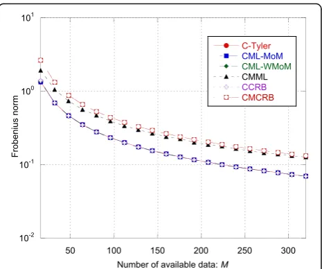
In this section, we compare the estimation performance of the matched CML-MoM estimator, the recursive CML-WMoM estimator, and the robust C-Tyler estima-tor with the CCRB, while the performance of the mis-matched CMML estimator are compared with the CMCRB. In order to have a global performance index (i.e., an index that is able to take into account the errors made in the estimation of all the covariance entries), we defineεas the Frobenius norm of the mean square error (MSE) matrix of the estimator [47]:

ε≜ E vecs Σ^ −vecsð ÞΣ vecs Σ^ −vecsð ÞΣ T

n o

F;

ð67Þ

where Σ^ is an estimate of the true covariance matrixΣ (e.g., εC‐Tyler, εCML‐MoM, εCML‐WMoM, and εCMML) and

A

k k_F ¼ ffiffiffiffiffiffiffiffiffiffiffiffiffiffiffiffiffiffitr ATA

q

is the Frobenius norm of matrixA. As performance bounds, the following quantity are plotted:

εCCRB≜kCCRBð ÞΣ kF; εCMCRB≜kCMCRBð ÞΣ kF:

ð68Þ

The accuracy on the estimate of the shape λand scale η parameters in the matched case and of the average power σ2in the mismatched case is measured through their MSE, which is compared with the CCRB and the CMCRB, respectively. To calculate the estimation accur-acy, we run 105 Monte Carlo trials. The simulation results have been organized as follows:

1. Estimation accuracy as function of the numberMof available data vectors (Figs.1,2,3, and4). Simulation parameters:ρ= 0.8,N= 16,λ= 3,η= 1,K= 4. 2. Estimation accuracy as function of the shape parameterλ(Figs.5,6,7, and8). Simulation parameters:ρ= 0.8,N= 16,M= 10N,η= 1,K= 4. 3. Estimation accuracy as function of the one-lag

correlation coefficient ρ (Figs. 9, 10, 11, and12). Simulation parameters:N= 16, M= 10N, λ= 3,

η= 1, K= 4.

Based on the numerical analysis, we observe that:

Regarding the scatter matrix estimation, the robust C-Tyler estimator is an“almost”efficient estimator, even if it is not the most efficient estimator for t-distributed data, in fact when λ increases, the other two estimators achieve better performance. The MSE εC‐Tyler is close to the CCRB especially

for small λ (see Figs. 1, 5, and9). In particular, its performance is robust, i.e., it is not affected by the value of the shape parameter λ (see Fig. 5), even if it is not efficient for large λ.

Regarding the CMML estimator, it always achieves the CMCRB, both for the scatter matrix estimation and for the estimation of the average power (see Figs.1,5,8,9, and12). The CMML presents a small bias on the estimation of the scatter matrix and then,Σ^CMMLis not aMS-unbiased estimator [9] (at least in the finite sample regime). For this reason,

εCMMLis in general slightly below the CMCRB. The

loss in estimation accuracy due to the mismatch is particularly high for extremely heavy-tailed data, i.e., whenλis close to 0 (see Fig.5). Whenλ→0, the CMCRB rapidly increases while the CCRB is quite independent ofλ. On the other hand, whenλ→∞, the CMCRB and the CCRB coincide, as expected, and the performance of the CMML estimator converge to that of the CML-MoM and CML-WMoM estimators.

Quite surprisingly, even if the MoM-based estimators fail to provide an accurate estimate ofλas it increases (see Fig. 6), the MSE of the CML-MoM and CML-WMoM estimators achieve the CCRB, as shown in Fig. 5.

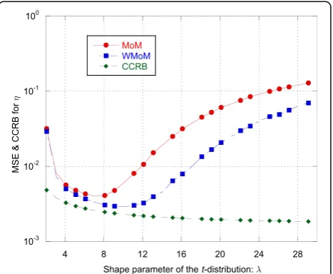
Regarding the estimation ofλandη, the recursive WMoM estimator always outperforms the classical MoM estimator (see Figs.2,3,7,10, and11), even though it does not achieve the CCRB. In particular, as shown in Fig. 10, the MSE of the WMoM is independent from the value of ρ, while this is not the case for the MSE of the classical MoM estimator. This desirable behavior of the WMoM estimator is due to the whitening operation that makes each entry of the data vectors mutually uncorrelated, as discussed in Section 3.1.

Fig. 1MSE indices εC-Tyler,εCML-MoM,εCML-WMoM, andεCMMLand

boundsεCCRBandεCMCRBas function of the numberMof available

5.2 Detection performance

In this section, the detection performance of the matched LTD detector, which exploits either the CML-MoM or the CML-WCML-MoM estimators, the mismatched Kelly’s GLRT, and the robust ANMF, that relies on the robust C-Tyler's estimator, are investigated. In particular, we analyze:

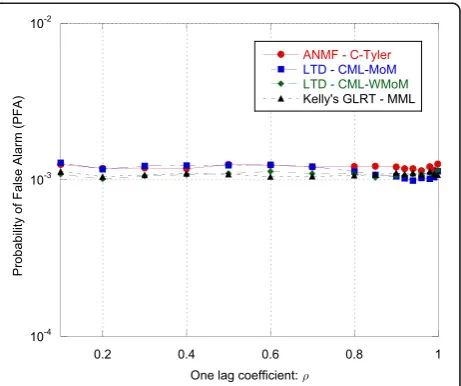
1. The probability of false alarm (PFA) as function of

the one-lag coefficientρ(Fig.13). This allows us to verify the CFAR property of theΛLTD‐CML‐MoM

(Eq. (59)),ΛLTD‐CML‐WMoM(Eq. (60)),ΛKelly(Eq.

(63)), and ΛANMF‐C‐Tyler (Eq. (66)) w.r.t. the

correlation shape. Simulation parameters: N= 16,

M= 3N,λ= 3,η= 1,K= 4. The detection thresholds have been set to achieve a nominalPFAof 10−3.

2. The probability of false alarm (PFA) as function

of the shape parameter λ of the true complex t-distribution, i.e., for different spikiness levels (Fig. 14). This is important, since it highlights the CFARness of the four detectors w.r.t. the non-Gaussianity level of the data. Simulation parameters:N= 16,M= 3N, ρ= 0.8, η= 1, K= 4. The detection thresholds have been set to achieve a nominalPFA of 10−3.

3. The receiver operating characteristic (ROC) curves (Fig.15). The simulation parameters are the following:N= 16,M= 3N,ρ= 0.8,λ= 3,η= 1, and K= 4. Moreover,α∼CN 0;σ2_αwhereσ2_αis set to have signal to noise power ratio (SNR) equal to 3 dB.

Fig. 2MSE and CCRB on the estimate of the shape parameterλas

function of the numberMof available data vectors

Fig. 3MSE and CCRB on the estimate of the scale parameterηas

function of the numberMof available data vectors

Fig. 4MSE of the CMML estimator ofσ2_{and CMCRB as function of}

the numberMof available data vectors

Fig. 5The MSE indicesεC-Tyler,εCML-MoM,εCML-WMoM, andεCMMLand

As we can see from Fig. 13, all the analyzed detectors are CFAR with respect to ρ. Their PFA curves are con-stant and close to the nominal value 10−3. A different behavior can be observed in Fig. 14, where the PFA curves have been evaluated as function of λ. It can be noted that onlyΛANMF‐C‐Tyleris a CFAR detector w.r.t. the data spikiness, while the PFA of the other detectors change with λ. Finally, in Fig. 15, the ROC curves of ΛLTD‐CML‐MoM, ΛLTD‐CML‐WMoM, ΛKelly ' s GLRT, and ΛANMF‐C‐Tyler are shown. For the sake of comparison, we evaluated also the ROC of the clairvoyant optimum detector for the t-distributed data, i.e., the ΛLTD in Eq. (58) where Σ, λ, and ηare perfectly known. As we can see, the performance of ΛLTD‐CML‐MoM, ΛLTD‐CML‐

WMoM, andΛANMF‐C‐Tylerare close to that of the clair-voyant detector ΛLTD, while ΛKelly ' s GLRT undergoes some detection loss for relatively low value of the PFA. In particular, the fact that the performance of the robust ΛANMF‐C‐Tyler is close to the one of the matched detec-tors, ΛLTD‐CML‐MoM and ΛLTD‐CML‐WMoM, suggests that the detection loss due to the robustness is small. However, it must be highlighted again that we are considering a particular scenario in which the clutter covariance matrix is assumed to be real and full rank. Moreover, due to the high computational load of the Monte Carlo simulations, the detection performance of the proposed detectors has been evaluated only for aPFA greater that 10−5. It would be very useful to investigate

Fig. 6MSE and CCRB on the estimate of the shape parameterλas

function ofλ

Fig. 7MSE and CCRB on the estimate of the scale parameterηas

function of the shape parameterλ

Fig. 8MSE of the CMML estimator ofσ2and CMCRB as function of

the shape parameterλ

Fig. 9The MSE indicesεC-Tyler,εCML-MoM,εCML-WMoM, andεCMMLand

the boundsεCCRBandεCMCRBas function of the one-lag correlation

the detection performance at an operative value of PFA, e.g., below 10−5.

6 Conclusions

This paper focused on two inference problems, the scat-ter matrix estimation and the adaptive detection of radar targets in complext-distributed data. Three different ap-proaches have been investigated and compared: the matched, the mismatched, and the robust approaches. Regarding the classical matched approach, we analyzed the performance of the CML estimator for the scatter matrix, when the shape and scale parameters are esti-mated through the low-complexity and suboptimal MoM method (CML-MoM) and a recursive improve-ment of it (CML-WMoM). We found that both the

CML-MoM and the CML-WMoM estimators achieve the CCRB, while the CML-WMoM estimator outper-forms the CML-MoM for the estimation of the shape and scale parameters. Then, the previous two estimators have been adapted to implement the LTD, which is the GLRT decision rule int-distributed data. Numerical sim-ulations show that the performance of the adaptive LTD are very close to the clairvoyant LTD detector, but it is not CFAR w.r.t. the variation of data spikyness. Regard-ing the mismatched approach, we proved that the CMML estimator derived under the assumption of Gaussian-distributed data converges almost surely to the true scatter matrix and to the true (t-distributed) data power, so it can be applied for inference problems that require the knowledge of these two quantities. Moreover,

Fig. 10MSE and CCRB on the estimate of the shape parameterλas

function ofρ

Fig. 11MSE and CCRB on the estimate of the scale parameterηas

function ofρ

Fig. 12MSE of the CMML estimator ofσ2_{and CMCRB as function of}

the one-lag correlation coefficientρ

its efficiency with respect to the CMCRB has been shown and its performance loss with respect to the matched case discussed. The CMML estimator of the scatter matrix has been used in the“mismatched”Kelly’s GLRT. Numerical simulations proved that Kelly’s GLRT is not CFAR and presents large performance loss for small values ofPFA. Finally, the min-max robust C-Tyler scatter matrix estimator and the adaptive version of the robust NMF detector, that exploits the C-Tyler estima-tor, have been introduced and analyzed. In particular, our numerical results demonstrated that Tyler’s estima-tor is an“almost”efficient estimator w.r.t. the CCRB and its estimation accuracy is independent on the value of the shape parameter. More importantly, the resulting ANMF is CFAR w.r.t. the shape parameter, i.e., w.r.t. the level of data spikiness, and has only a small detection loss

w.r.t. the clairvoyant LTD. To summarize, the results discussed in this paper show that the robust approach, thanks to its generality, robustness to misspecification, and small estimation and detection losses, seems to be the a good choice in practical applications.

Competing interests

The authors declare that they have no competing interests.

Received: 7 July 2016 Accepted: 29 October 2016

References

1. H Krim, M Viberg, Two decades of array signal processing research: the parametric approach. IEEE Signal Process. Mag.13(4), 67–94 (1996) 2. J Karhunen, J Joutsensalo, Generalizations of principal component analysis,

optimization problems, and neural networks. Neural Netw.8(4), 549_–562 (1995) 3. O Ledoit, M Wolf, Improved estimation of the covariance matrix of stock

returns with an application to portfolio selection. J. Empir. Finance10(5), 603–621 (2003)

4. CD Richmond,Adaptive array signal processing and performance analysis in non-Gaussian environments. Ph.D. thesis (MIT, Cambridge, MA, 1996). Available at: https://dspace.mit.edu/handle/1721.1/11005

5. E Ollila, DE Tyler, V Koivunen, VH Poor, Complex elliptically symmetric distributions: survey, new results and applications. IEEE Trans. Signal Process.60(11), 5597–5625 (2012)

6. KL Lange, RJA Little, JMG Taylor, Robust statistical modeling using the tdistribution. J. Am. Stat. Assoc.84(408), 881–896 (1989)

7. JP Romano, AF Siegel,Counterexamples in probability and statistics, Wadsworth and Brooks/Cole, Monterey, CA

8. S Fortunati, MS Greco, F Gini, The impact of unknown extra parameters on scatter matrix estimation and detection performance in complext -distributed data,IEEE Workshop on Statistical Signal Processing 2016 (SSP), (IEE, Palma de Mallorca, 2016), pp 1–4. doi:10.1109/SSP.2016.7551738 9. S Fortunati, F Gini, MS Greco, On scatter matrix estimation in the presence

of unknown extra parameters: mismatched scenario,EUSIPCO 2016, (Budapest, Hungary, 2016)

10. A Balleri, A Nehorai, J Wang, Maximum likelihood estimation for compound-Gaussian clutter with inverse gamma texture. IEEE Trans. Aerosp. Electron. Syst.43(2), 775–779 (2007)

11. J Wang, A Dogandzic, A Nehorai, Maximum likelihood estimation of compound-Gaussian clutter and target parameters. IEEE Trans. Signal Process.54(10), 3884–3898 (2006)

12. KJ Sangston, F Gini, MS Greco, Coherent radar target detection in heavy-tailed compound-Gaussian clutter. IEEE Trans. Aerosp. Electron. Syst.48(1), 64_–77 (2012) 13. A Younsi, M Greco, F Gini, A Zoubir, Performance of the adaptive generalised

matched subspace constant false alarm rate detector in non-Gaussian noise: an experimental analysis. IET Radar Sonar Navigation3(3), 195–202 (2009) 14. S Fortunati, F Gini, MS Greco, The misspecified Cramér-Rao bound and its

application to the scatter matrix estimation in complex elliptically symmetric distributions. IEEE Trans. Signal Process.64(9), 2387–2399 (2016) 15. S Fortunati, F Gini, MS Greco, The constrained misspecified Cramér-Rao

bound. IEEE Signal Process. Lett.23(5), 718_–721 (2016)

16. D Tyler, A distribution-free M-estimator of multivariate scatter. Ann. Stat.

15(1), 234–251 (1987)

17. EJ Kelly, An adaptive detection algorithm. IEEE Trans. Aerosp. Electron. Syst.

AES-22(2), 115_–127 (1986)

18. LL Scharf, B Friedlander, Matched subspace detectors. IEEE Trans. Signal Process.42(8), 2146–2157 (1994)

19. F Gini, A cumulant-based adaptive technique for coherent radar detection in a mixture of K-distributed clutter and Gaussian disturbance. IEEE Trans. Signal Process.45(6), 1507–1519 (1997)

20. E Conte, A De Maio, G Ricci, Recursive estimation of the covariance matrix of a compound-Gaussian process and its application to adaptive CFAR detection. IEEE Trans. Signal Process.50(8), 1908_–1915 (2002)

21. F Gini, Sub-optimum coherent radar detection in a mixture of k-distributed and Gaussian clutter. IEE Proc. Part F144(1), 39–48 (1997)

22. F Gini, MV Greco, A Farina, Clairvoyant and adaptive signal detection in non-Gaussian clutter: a data-dependent threshold interpretation. IEEE Trans. on Signal Processing47(6), 1522–1531 (1999)

Fig. 14Probability of false alarm vsλ

ANMF - C-Tyler

LTD - CML-MoM LTD - CML-WMoM Kelly's GLRT - MML

Clairvoyant LTD

23. F Gini, MV Greco, A suboptimum approach to adaptive coherent radar detection in compound-Gaussian clutter. IEEE Trans. Aerosp. Electron. Syst.

35(3), 1095–1104 (1999)

24. E Ollila, DE Tyler, V Koivunen, HV Poor, Compound-Gaussian clutter modelling with an inverse Gaussian texture distribution. IEEE Signal Processing Letters

19(12), 876_–879 (2012)

25. A Farina, F Gini, MV Greco, L Verrazzani, High resolution sea clutter data: statistical analysis of recorded live data. IEE Proc. Radar Sonar Navigation

144(3), 121–130 (1997)

26. R Remmer,Theory of complex functions(Springer-Verlag, New York, NY, USA, 1991)

27. MS Greco, F Gini, Cramér-Rao lower bounds on covariance matrix estimation for complex elliptically symmetric distributions. IEEE Trans. Signal Process.

61(24), 6401_–6409 (2013)

28. P Stinco, MS Greco, F Gini,Adaptive detection in compound-Gaussian clutter with inverse-gamma texture. IEEE CIE International Conference on Radar 2011, 2011, pp. 434–437

29. MS Greco, S Fortunati, F Gini,Naive, robust or fully-adaptive: an estimation problem for CES distributions. 8-th IEEE Sensor Array and Multichannel Signal Processing Workshop (SAM 2014), 2014, pp. 457–460

30. JR Magnus, H Neudecker, The commutation matrix: some properties and applications. Ann. Stat.7, 381_–394 (1979)

31. JD Gorman, AO Hero, Lower bounds for parametric estimation with constraints. IEEE Trans. Inf. Theory6(6), 1285–1301 (1990)

32. P Stoica, BC Ng, On the Cramer-Rao bound under parametric constraints. IEEE Signal Processing Letters5(7), 177_–179 (1998)

33. CD Richmond, LL Horowitz, Parameter bounds on estimation accuracy under model misspecification. IEEE Trans. on Signal Processing63(9), 2263–2278 (2015)

34. PJ Huber,The behavior of maximum likelihood estimates under nonstandard conditions. Proc. of the Fifth Berkeley Symposium in Mathematical Statistics and Probability (University of California Press, Berkley, 1967)

35. H White, Maximum likelihood estimation of misspecified models. Econometrica50, 1_–25 (1982)

36. CC Heyde, R Morton, On constrained quasi-likelihood estimation. Biometrika

80(4), 755–61 (1993)

37. QH Vuong, Cramér-Rao bounds for misspecified models,Working paper 652, Division of the Humanities and Social Sciences(Caltech, 1986). Available at: https://www.hss.caltech.edu/content/cramer-rao-bounds-misspecified-models 38. MS Greco, S Fortunati, F Gini, Maximum likelihood covariance matrix estimation for complex elliptically symmetric distributions under mismatched conditions. Signal Process.104, 381_–386 (2014)

39. RA Maronna, Robust M-estimators of multivariate location and scatter. Ann. Stat.4(1), 51–67 (1976)

40. F Gini, MS Greco, Covariance matrix estimation for CFAR detection in correlated heavy tailed clutter. Signal Process.82(12), 1847_–1859 (2002) 41. F Pascal, Y Chitour, J Ovarlez, P Forster, P Larzabal, Covariance structure

maximum-likelihood estimates in compound Gaussian noise: existence and algorithm analysis. IEEE Trans. Signal Process.56(1), 34–48 (2008) 42. M Skolnik,Introduction to radar systems: third edition(McGraw-Hill, New

York, 2001)

43. CD Richmond, A note on non-Gaussian adaptive array detection and signal parameter estimation. IEEE Trans. on Signal Processing3(8), 251–252 (1996) 44. NB Pulsone, RS Raghavan, Analysis of an adaptive CFAR detector in

non-Gaussian interference. IEEE Trans. Aerosp. Electron. Syst.35(3), 903–916 (1999) 45. F Pascal, JP Ovarlez, Asymptotic detection performance of the robust ANMF,

23rd European Signal Processing Conference(EUSIPCO), 2015, Nice, 2015, pp. 524-528

46. JP Ovarlez, F Pascal, A Breloy, Asymptotic detection performance analysis of the robust adaptive normalized matched filter,IEEE CAMSAP 2015, (Cancun, 2015), pp. 137-140

47. F Gini, JH Michels, Performance analysis of two covariance matrix estimators in compound-Gaussian clutter. IEE Proceedings Part-F146(3), 133–140 (1999)

Submit your manuscript to a

journal and benefi t from:

7 Convenient online submission

7 Rigorous peer review

7 Immediate publication on acceptance

7 Open access: articles freely available online

7 High visibility within the fi eld

7 Retaining the copyright to your article