R E S E A R C H
Open Access
A traffic data collection and analysis
method based on wireless sensor network
Huan Wang
1*, Min Ouyang
2, Qingyuan Meng
1and Qian Kong
1Abstract
With the rapid development of urbanization, collecting and analyzing traffic flow data are of great significance to build intelligent cities. The paper proposes a novel traffic data collection method based on wireless sensor network (WSN), which cannot only collect traffic flow data, but also record the speed and position of vehicles. On this basis, the paper proposes a data analysis method based on incremental noise addition for traffic flow data, which provides a criterion for chaotic identification. The method adds noise of different intensities to the signal incrementally by an improved surrogate data method and uses the delayed mutual information to measure the complexity of signals. Based on these steps, the trend of complexity change of mixed signal can be used to identify signal characteristics. The numerical experiments show that, based on incremental noise addition, the complexity trends of periodic data, random data, and chaotic data are different. The application of the method opens a new way for traffic flow data collection and analysis.
Keywords:Traffic data collection, Wireless sensor network, Incremental noise addition, Noise intensity, Delayed mutual information
1 Introduction
Traffic congestion is a daily phenomenon in large- and medium-sized cities all over the world. With limited urban facilities and resources, it is an effective way to control traffic congestion by analyzing and predicting traffic flow. This involves two issues, collecting and ana-lyzing traffic data.
There are many methods to collect traffic data, such as pneumatic road tubes [1], induction loop [2], and piezoelectric sensors [3]. These methods can collect traffic flow, but cannot record the speed and location of vehicles, which cannot meet the needs of traffic flow analysis algo-rithm. The paper proposes a novel traffic data collection scheme based on wireless sensor network (WSN). The scheme measures vehicle flow and speed based on vehicle disturbances to geomagnetism and uses the slotted ALOHA protocol to communicate between data nodes. Based on the scheme, vehicle speed and location are record every specific time slot.
Chaos algorithm is widely used in traffic flow data processing, and chaotic identification is the premise of chaotic analysis. However, because of the complexity of chaos, its intrinsic mechanism has not been fully re-vealed, so the academic community has not yet proposed a unified definition of chaos. Aiming at the chaotic iden-tification, scholars have proposed many criterions, such as Poincare section [4], bifurcation diagram [5], power spectrum [6], Kolmogorov entropy [7], and topological entropy [8]. The most commonly used criteria are the largest Lyapunov exponent [9,10] and the fractal dimen-sion [11, 12], but these two parameters are based on phase space reconstruction [13, 14]. Only in real phase space or near-real phase space that the two parameters can accurately analyze and identify the signal. The time delay method based on the Takens embedding theorem [15] is a main way for phase space reconstruction. How-ever, this method has been influenced by many causes in practice, so the real phase space model of the object is often difficult to get, which leads to the unreliability of the identification results.
According to the idea of indirect method, the noise of different intensities is incrementally added to the signal, and it is found that the complexity trend of the mixed
© The Author(s). 2019Open AccessThis article is distributed under the terms of the Creative Commons Attribution 4.0 International License (http://creativecommons.org/licenses/by/4.0/), which permits unrestricted use, distribution, and reproduction in any medium, provided you give appropriate credit to the original author(s) and the source, provide a link to the Creative Commons license, and indicate if changes were made.
* Correspondence:[email protected]
1Zhongshan Institute, University of Electronic Science and Technology of China, Zhongshan 528400, China
signal is an important feature for identifying signal char-acteristics. The paper uses surrogate data method as a noise-adding algorithm, and the noise intensity ρ in the algorithm is used to measure the size of adding noise. Then the delayed mutual information is used to measure the complexity of signals. The numerical experiments show that, based on incremental noise addition, the complexity trends of periodic data, random data, and chaotic data are different. This feature can be used as a significant criterion for identifying the differences of various kinds of signals, which achieves reliable chaotic recognition for traffic flow signals.
2 Traffic data collection scheme based on WSN 2.1 System architecture
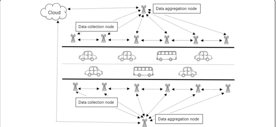
The scheme uses a magnetometer to count the vehicle and identify the speed. Normally, the Earth’s magnetic field is almost evenly distributed anywhere on the sur-face, between 0.25 and 0.65 gauss. Since the vehicle is generally composed of a highly permeable ferrous mater-ial, when the vehicle passes through the sensor, it dis-turbs the Earth’s magnetic field in the detection area. Generally, a magnetometer sensor can detect vehicles that are 10 m apart. The system architecture is shown in Fig. 1. In the system, all data collection nodes are re-sponsible for collecting road traffic data, and then these nodes transmit data to the aggregation node based on the ALOHA protocol and finally transmit to the remote server through the mobile internet. The system has strong scalability, and the cost of construction,
maintenance and operation is low, which is suitable for urban traffic monitoring.
2.2 Hardware selection
The data collection node uses RFM69HCW wireless module and magnetometer sensor FXOS8700CQ to build the hardware part. RFM69HCW is a low-cost, ver-satile radio module that can work in the unauthorized ISM (industrial, scientific, and medical) band. RF69 is a wireless transceiver chip promoted by HopeRF. It has + 20 dBm transmission power, −120 dBm sensitivity, and 140 dB link budget. The module operates at 915 MHz with a maximum spatial rate of 300 kbps. RFM69HCW uses SPI (Serial Peripheral Interface) to communicate with the master microcontroller and provides several Arduino libraries. It supports up to 256 networks, each with 255 nodes, and uses AES encryption to protect your data without restriction and transmits up to 66 bytes of packets. The module costs less than $2 and consumes less power to support on-board power supply.
The FXOS8700CQ is a smart digital chipset that inte-grates a three-axis magnetometer and a three-axis accel-erometer sensor. The three-axis magnetometer has a dynamic detection range of 1200 μT and a 16-bit ADC resolution with a sensitivity of 0.1 μT/LSB. Power con-sumption is as low as 8μA and consumes only 2μA in standby mode. The chip has a wide measurement range, high resolution, low noise density, high sensitivity, low output noise range, low cost, low power consumption, and the ability to manage high interference areas.
2.3 Wireless communication protocol
ALOHA protocol is selected in this scheme. ALOHA is the earliest and most basic wireless data communication protocol. Its idea is simple. As long as users have data to send, let them send it. Usually, it includes pure ALOHA protocol and slotted ALOHA protocol.
Pure ALOHA is the most basic form of a MAC proto-col, it has two rules:
If there is data to be sent, send the data.
And if, while sending that data, the data is received from another node, a collision has occurred. If this happens, try resending the data later.
This protocol is seldom used because of its high chan-nel conflict.
Slotted ALOHA is an improved vision of pure ALOHA, which modifies the protocol by adding slots that dictate when a node may start transmitting. Adding the rule doubles the throughput of the protocol to a suc-cessful transmission rate of 36%. Therefore, the slotted ALOHA protocol is chosen in this scheme.
3 Traffic data analysis method
Chaos theory is an effective method of data analysis, but the premise of chaos analysis is chaos identification. A data analysis method based on incremental noise addition is proposed in the paper for traffic flow data, which provides a criterion for chaotic identification. The method uses an improved surrogate data method to add noise to the signal to be analyzed incrementally, while using delayed mutual information to measure the com-plexity of mixing signals under different noise intensity.
3.1 Noise addition: Pseudo-periodic surrogate data method
3.1.1 The basic steps of pseudo-periodic surrogate data method
The pseudo-periodic surrogate data method (PPS) [16] is proposed by Small in 2001 and has been successfully applied to the chaotic identification of ECG signals. The essence of this method is to add noise to the source signal by changing the signal phase order.
The main steps of the PPS algorithm are as follows: Step 1: For time series {x(t),t= 1, 2,⋯,N}, the phase space is reconstructed according to the Takens embed-ding theorem and generates a set of high dimension vec-torX= {X1,X2,⋯,XL},
Xt ¼fx tð Þ;x tð þτÞ;⋯;x t½ þðm−1ÞτÞgt
¼1;2;⋯;L ð1Þ
In formula (1), m is embedding dimension, τ is time delay, andL=N−(m−1)τ.
Step 2: Select a phase points1randomly in phase space
Xas the first value of vector sequenceS,s1∈X;
Step 3: According to the Euclidean distance between
s1and phase points in phase spaceX, calculate the tran-sition probability of phase points and select s2randomly according to this probability, and so on. The transition probability is set as
Probðsiþ1¼XtÞ∝exp− Xt−si
k k
ρ ð2Þ
In formula (2), ρ is the noise intensity, which is a key parameter, and its significance will be discussed in the later paper.
Step 4: Repeats the steps until select vector sequence
S= {s1,s2,⋯sN}, and the surrogate data ~S is a time series which is composed of the first coordinate of each phase point in vector sequence S.
3.1.2 The discussion of pseudo-periodic surrogate data method
The PPS has three parameters, which are embedding di-mensionm, time delayτ, and noise intensityρ. However, the value ofρis the key to randomly changing the phase sequence of the source signal, and the choice ofmandτ has no large effect on the algorithm. Therefore, the algo-rithm does not need phase space reconstruction, and m and τneed only to specify as a fixed set of values. Ac-cording to formula (2), when ρvalue is small, the phase transition probability is small, the phase point in the vector sequence S can only jump around the initial phase points1, so the surrogate data is similar to the ori-ginal data; When ρ increases gradually, the transition probability increases gradually too, and the jump range of the phase point in S increases accordingly. When ρ increases to a certain extent, the phase point in S will jump randomly in phase space X, so surrogate data ~S will be a completely random signal. Therefore, the ρ value determines the amplitude of noise added to the source signal in PPS. It is especially pointed out that, the
ρvalue is associated with the value of the original signal, so before the analysis, it is necessary to normalize the original signal.
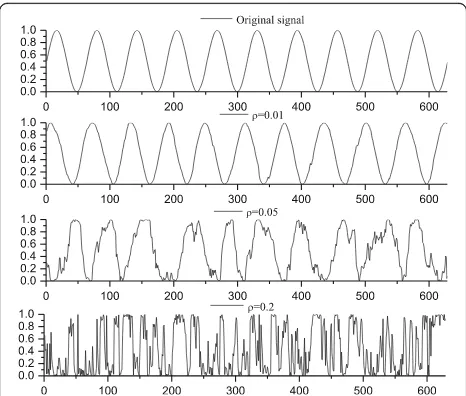
According to the PPS, the surrogate data of a sine sig-nal under each noise intensity are shown in Fig.2.
sine signal gradually evolve from a regular sequence to a random sequence.
In summary, PPS can be used as a noise addition algo-rithm. Compared with the method of adding white noise, this algorithm can disrupt the phase order of the original data. With the increase of ρ, the structure of original data is gradually annihilated, but at the same time, the mean, variance, and range of the signals remain unchanged. Randomizing the signal while preserving the statistical characteristics is an important feature of the algorithm.
3.2 The parameter for signal complexity evaluation After adding the quantitative noise to the signal, it is ne-cessary to evaluate the complexity of the signal with noise effectively. Kolmogorov proposed the first defin-ition of the signal complexity in 1965. Later, Lempel and Ziv proposed the specific algorithm called LZ complex-ity, which is widely used in the research of nonlinear science. In addition, Skyllingstad et al. [17] studied the correlation between the delayed mutual information and entropy then drew the conclusion the slope of mutual information is negatively correlated with the entropy. Therefore, delayed mutual information is also often used to measure the complexity of a time series. Taking the logistic chaotic time series, Lorenz’s chaotic time series, and ECG signals as examples, Zhang [18] compares LZ complexity and delayed mutual information. The con-clusion is that both parameters can effectively express the data complexity, and the values are negatively corre-lated. Calculating the two parameters using a
four-segment or more detailed four-segmentation algorithm can more accurately reflect the essence of nonlinear signals. The example analysis shows the delayed mutual infor-mation is more sensitive than the LZ complexity in ex-pressing the intrinsic characteristics of the nonlinear dynamic system. Therefore, this paper uses delayed mu-tual information as the measurement for the signal complexity.
3.2.1 The definition of mutual information
AandBare the two information systems, the state space of the two systems are respectivelyA= {a1,a2,⋯,an} and
B = {b1,b2,⋯,bm}, and the corresponding probabilities in
the state spaces are p(ai)(i= 1, 2,⋯,n) and p(bj)(j= 1, 2, ⋯,m), among themP
n
i¼1
pðxiÞ ¼1 andP m
j¼1
pðxjÞ ¼1.Aand
B can be regarded as two information sources, and their respective information entropy are
H Að Þ ¼−Xni¼1p að Þi log2p að Þ2 ð4Þ
H Bð Þ ¼−Xmj¼1p bj log2p bj ð5Þ
The joint information source AB is composed of A and B, and its state space is AB = {a1b1,a1b2,⋯,anbm},
and the joint probability distribution corresponding to the state space is
a1b1 a1b2 ⋯ anbm p að 1b1Þ p að 1b1Þ ⋯ p að nbmÞ
ð6Þ
The information entropy of the joint source AB is
HðABÞ ¼−Xni¼ 1
Xm j¼1p aibj
log2 a2bj
ð7Þ
The mutual information of the sourcesAandB is de-fined as
MIðA;BÞ ¼H Að Þ þH Bð Þ−HðABÞ ð8Þ
Mutual information can express the correlation be-tween two sources A and B. When Ais the same as B, the value of mutual information is maximum; when A and B are independent of each other, the mutual infor-mation is 0.
3.2.2 Calculation of delayed mutual information
To express the complexity of a signal, the time series of a signal can be used to calculate the delayed mutual in-formation. Time series A= {a1,a2,⋯,an} can be
regarded as the information source A, moves the se-quence of source A backward for the k points, and the times series B= {a1 +k,a2 +k,⋯,an+k} is obtained, which can be regarded as the information source B. The mu-tual information betweenAandBis called delayed mu-tual information of a signal. The specific algorithms are
Fig. 2Sine signal and the surrogate data under different noise intensity. Add noise of different intensities (corresponding to the value of parameterρ) to a sine signal using the PPS algorithm. With the increase of noise, the structure of source signal is
as follows: The ranges ofAandBare divided into 2c sec-tions evenly from the minimum to the maximum, then 1, 2, ⋯, i, ⋯, 2c and 1, 2, ⋯, j, ⋯, 2c are used as the scale of each section, respectively. The joint information source AB can be regarded as a two-dimension vector; the corresponding sections of the two-dimension vector can be labeled by (i,j), i, j= 1, 2, ⋯, 2c; the scales of these sections are (1, 1), (1, 2),⋯, (2, 1),⋯, (i, j),⋯, (2c, 2c); and the total quantity of these sections is 22c. Counts the number num(i,j) of the joint information source AB in the section (i,j), and calculates the joint probability of corresponding section (i,j) as below
p a ibj¼numnð Þi;j ;ði;j¼1;2;⋯;2cÞ ð9Þ
nis the total number of the time series data, then
p að Þ ¼i
X2c
j¼1
numð Þi;j
n ¼
numð Þi
n ð10Þ
p bj ¼
X2c
i¼1
numð Þi;j
n ¼
numð Þj
n ð11Þ
Sets the delay pointk= 0, 1, 2,⋯,K, and brings the cal-culation results of formulas (9), (10), and (11) into formulas (4), (5), (7), and (8), then the delayed mutual information sequence D= {D0,D1,⋯,DK} of time series A can be
ob-tained. When k = 0, the time seriesAandBare exactly the same, and the time delay mutual information D0is max-imum, that is,D0≥Dl,D= 1, 2,⋯,K. Therefore, the value ofD0can be used to normalizeI. Applying the algorithm, the delayed mutual information sequences of a Lorenz cha-otic signal and a periodic signal are shown in Fig.3.
In Fig. 3, with the increase of time delay, the delayed mutual information value of the Lorenz chaotic signal decreases rapidly and then keeps oscillating between [0.1,0,3]; meanwhile, the delayed mutual information value of the periodic signal oscillates between [0.75,1] periodically. The figure shows the delayed mutual infor-mation oscillations range of high complexity chaotic sig-nals are far lower than the periodic sigsig-nals’ with lower complexity, which shows the complexity of signal can be expressed by delayed mutual information. To quantify the complexity accurately, this paper uses the mean value MD ofK+ 1 delayed mutual information fromk= 0 toKas the measurement:
MD¼ PK
i¼1Di
Kþ1 ð12Þ
4 Result and discussion 4.1 Data sources
In this section, the method of the third section is used to carry out numerical experiments on typical periodic signals, chaotic signals, and random signals, respectively.
The periodic signals used for analysis are generated by logistic model [19]. The logistic model, proposed by biologist May, is also called model of insect, which is the most prestigious achievement in the early study of chaos. The expression of the model is
xnþ1¼λxnð1−xnÞ ð13Þ
In formula (13),n = 1,2,…, is the iterative sequence,λ is a key control parameter, and λ∈[3, 4], the iterative initial valuex0∈[0, 1]. The logistic model is a famous ex-ample from regularity to chaos. The model can produce typical periodic signals and chaotic signals by setting dif-ferent values ofλ. Using the logistic model, three sets of periodic signals are generated, which λ values are 3.4, 3.84, and 3.5, and the three sets of signals are double period, triple period, and four times period, respectively.
There are two groups of chaotic signals for analysis. The three chaotic signals in the first group are also gen-erated by logistic model, whichλvalues are 3.7, 3.8, and 3.9, respectively. The two signals in the second group are generated by the Lorenz attractor [20] and Henon attractor [21]. In addition, to analyze the signal charac-teristics, a set of traffic flow data is selected in the sec-ond group.
Finally, three white Gaussian noise signals are selected as random signals for numerical analysis.
All the signals used for analysis above can be regarded as time series, and all of which have a length of 5000.
4.2 Experimental design
For the above signals, the following analysis steps are adopted:
(1) The generation of surrogate data: First of all, the experimental signal is normalized. For the normalized signal, the noise intensity is set to be ρ= 0 : 0.01 : 0.2, then generates 5000 sets of surrogate data for eachρvalue respectively by means of improved PPS.
The calculation of MD: The range of the surrogate data under each noise intensity is divided into 32 sec-tions, that is 2c= 32, c= 5, then calculates the MD of each set of surrogate data. Finally, calculates the MD mean value of 5000 sets of surrogate data under each noise intensity.
(2) Draws the figure for the data from step 2 and discuss its connotation.
4.3 Experimental results and discussion 4.3.1 The periodic signals
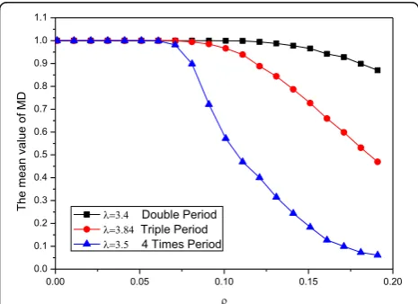
For three periodic signals, according to the experimental design, the surrogate data are generated separately, and then the corresponding MD values are calculated. After the above steps, the MD mean value curves of three sets of periodic sequences’ surrogate data under different noise intensity are shown in Fig.4.
According to Fig.4, when the noise intensityρ< 0.07, the values of the three curves are almost 1, and when the noise intensityρ> 0.07, the values of the three curves begin to descend to varying degrees. For the periodic signal, when the added noise is small, the signal is still
regular, and the complexity of the signal is not obviously changed. When the noise increases, the three curves range abilities are different, which is related to the struc-ture of these signals. The λvalues are 3.4, 3.84, and 3.5, and the periodic signals are double period, triple period, and three times period signal, respectively. With the in-crease of period multiplier, the structure of the periodic signal is more complex. The more complex the structure is, the more likely the signal is to be disturbed by noise. So in Fig. 4, when ρ> 0.07, the trend of the curve(λ= 3.4) is the slowest, while the trend of the curve (λ= 3.5) is the most intense.
4.3.2 The chaotic signals
Three chaotic signals in the first group are generated by the logistic model, and the MD mean value curves of these sequences’surrogate data under different noise in-tensity are shown in Fig.5.
Compared to Figs. 4 and 5, the trends of two sets of curves corresponding to periodic signals and chaotic sig-nals are remarkably different. First, the initial value of the three curves in Fig.5 is between [0.35,0.45], and the initial values of the three curves in Fig.4are all 1, which indicates that the complexity of the chaotic signal is much higher than that of the periodic signal. Second, with the increase of noise, three curves in Fig.5decrease monotonously. Theλ value of the three signals in Fig.5 can reflect the complexity of these signals. The higher the λ value, the more complex the signal is. Therefore, in Fig.5, the curve corresponding toλ= 3.7 is at the top, the curve corresponding to λ= 3.8 is centered, and the curve corresponding to λ= 3.9 is at the bottom. When the noise is large enough, the three sets of surrogate data almost turn into random signals, so the MD mean values of these signals tend to be consistent.
Fig. 4The MD mean value of three periodic signals’surrogate data. The curves corresponding to the periodic signals remain stable at first, and when the noise exceeds a certain threshold, these curves begin to decline
Fig. 5The MD mean value of first group chaotic signals’surrogate data. With the increase of noise, these curves decrease
The MD mean value curves corresponding to the three signals in the second group under different noise inten-sities are shown in Fig.6.
Compared to Figs. 5 and 6, although the curve values of the six sets of signals are different, the curve charac-teristics are very similar. In particular, the corresponding curve characteristic of the traffic flow signal is consistent with those of other chaotic signals.
4.3.3 The random signals
The MD mean value curves of these random signal se-quences’ surrogate data under different noise intensity are shown in Fig.7.
According to Fig. 7, the characteristic of random sig-nals curves is obviously different from that of periodic signals and chaotic signals. The first value is smaller than the periodic signal and the chaotic signal, and with the increase of noise, the curve trend does not change significantly with the increase of noise. This is because the inherent complexity of the random signal is high, so the first value of MD is small; the noise complexity added in the original signal is not significantly different from the original random signal. As the noise increases, the MD value will not vary significantly, and the curve trend is relatively flat.
4.3.4 The comparison of three kinds of signals
In order to compare the difference of three kinds of sig-nals, the vector angle is used as the similarity measure-ment. Each curve in Figs. 4, 5, 6, and 7 is treated as a vector, and the similarity between curves can be mea-sured by the vector angle. The parameter is defined as
A¼ arccos v1v2
v1
k kk kv2 ð14Þ
In formula (14), v1 and v2 are two vectors, and the unit ofAis degree. The smaller theAvalue is, the stron-ger the correlation between the vectors is.
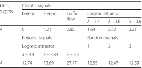
Takes the Lorenz signal curve as the reference, calcu-lates the vector angles of 12 curves in Figs.4,5,6, and7, the data are shown in Table1.
According to Table 1, the A values of chaotic signals are between [0∘, 3.5∘], which are significantly different from the A values of periodic signals and random sig-nals. Therefore, the surrogate data MD mean value changing trend under different noise intensities can be used as a strong criterion for distinguishing types of sig-nals. Meanwhile, it proves that traffic flow signal is a typical chaotic signal, which can be analyzed by chaotic theory. Of course, compared with the largest Lyapunov exponent and other parameters, the criterion proposed in this paper is relatively vague, and further work is needed.
Fig. 6The MD mean value of second group chaotic signals’ surrogate data. The curve trends of two groups of chaotic signals are highly consistent
Fig. 7The MD mean value of three random signals’surrogate data. The increase of added noise has no effect on the complexity of random signal, and the curves in the figure remain flat from beginning to end
Table 1Curve similarity analysis
Unit, degree
Chaotic signals
Lorenz Henon Traffic flow
Logistic attractor
λ= 3.7 λ= 3.8 λ= 3.9
A 0 1.21 2.85 1.64 2.32 3.21 Periodic signals Random signals
Logistic attractor 1 2 3
λ= 3.4 λ= 3.84 λ= 3.5
5 Conclusion
In this paper, a WSN-based traffic data collection scheme is proposed, which is low cost and low power. The scheme can collect vehicle speed and position infor-mation accurately and timely and lays a foundation for traffic flow analysis. Then a method based on incremen-tal noise addition is proposed for the chaotic identifica-tion of traffic flow signal. PPS is used to add noise incrementally to the analyzed signal, and the MD mean value is used as a measurement for the complexity of the signal. It is found that, for different types of signals, the complexity trends of surrogate data under each noise in-tensity are different. For the periodic signal, when the noise intensity is small, the MD mean value of surrogate data is stable; when the noise intensity is larger than a threshold, the MD mean value starts to decrease grad-ually. For the chaotic signal, such as traffic flow, the first MD mean value is obviously smaller than the periodic signal, and as the increase of noise intensity, the MD mean value keeps decreasing monotonously. For the ran-dom signal, the MD mean value keeps at a low value. Therefore, as the noise intensity increases, the trend of MD mean values is an effective criterion for distinguish-ing various types of signals. Of course, although param-eterAis used to try to quantify the criteria presented in this paper, the criterion is more inclined to a qualitative criterion than a quantitative one. Further research is needed to make extensive use of the criterion.
Abbreviations
ISM:Industrial, scientific and medical; MD: Mean value of delayed mutual information; PPS: Pseudo-periodic surrogate data method; SPI: Serial peripheral interface; WSN: Wireless sensor network
Authors’contributions
HW is the main author of the current paper. HW contributed to the development of the ideas, design of the study, theory, result analysis, and paper writing. MO contributed to the result analysis and paper revision. All authors read and approved the final manuscript.
Authors’information
HW received his Ph.D. degree in electrical engineering from Hunan University, China, in 2009. From 2010 to 2012, he was an electrical design engineer of Guangdong electric design institute, China. From 2012 till now, he is a lecturer at University of Electronic Science and Technology of China, Zhongshan Institute.
Funding
The work was supported by special innovation projects of universities in Guangdong Province, China (No.2018KTSCX), Hunan Provincial Natural Science Foundation of China (2018JJ2097).
Availability of data and materials Not applicable
Competing interests
The authors declare that they have no competing interests.
Author details
1Zhongshan Institute, University of Electronic Science and Technology of China, Zhongshan 528400, China.2School of Computer, Hunan University of Technology, Zhuzhou 412008, China.
Received: 31 July 2019 Accepted: 18 December 2019
References
1. G.S. Larue, C. Wullems, A new method for evaluating driver behavior and interventions for passive railway level crossings with pneumatic tubes [J]. J. Transportation Saf. Secur.11(2), 150–166 (2019)
2. M. Grote, I. Williams, J. Preston, et al., A practical model for predicting road traffic carbon dioxide emissions using Inductive loop detector data[J]. Transportation Res. Part D Transp. Environ.63, 809–825 (2018) 3. S. Rajab, M.O. Al Kalaa, H. Refai, Classification and speed estimation of
vehicles via tire detection using single-element piezoelectric sensor[J]. J. Adv. Transportation50(7), 1366–1385 (2016)
4. M. Zabihi, S. Kiranyaz, R.A. Bahrami, et al., Analysis of high-dimensional phase space via Poincaré section for patient-specific seizure detection [J]. IEEE Trans. Neural Syst. Rehabil. Eng.24(3), 386–398 (2015)
5. M.V. Ivanchenko, E.A. Kozinov, V.D. Volokitin, et al., Classical bifurcation diagrams by quantum means [J]. Annalen Der Physik529(8), 1600402 (2017) 6. A.S. Dmitriev, E.V. Efremova, N.V. Rumyantsev, A microwave chaos generator
with a flat envelope of the power spectrum in the range of 3–8 GHz [J]. Tech. Phys. Lett.40(1), 48–51 (2014)
7. Z. Hua, Y. Zhou, Image encryption using 2D logistic-adjusted-sine map [J]. Inf. Sci.339, 237–253 (2016)
8. N.V. Kuznetsov, G.A. Leonov, T.N. Mokaev, et al., Finite-time Lyapunov dimension and hidden attractor of the Rabinovich system [J]. Nonlinear dynamics92(2), 267–285 (2018)
9. J. Maldacena, S.H. Shenker, D. Stanford, A bound on chaos [J]. J. High Energy Phys.2016(8), 106 (2016)
10. W. Liu, K. Sun, C. Zhu, A fast image encryption algorithm based on chaotic map [J]. Opt. Lasers Eng.84, 26–36 (2016)
11. Y.W. Shon, The pattern recognition system using the fractal dimension of chaos theory [J]. Int. J. Fuzzy Logic Intell. Syst.15(2), 121–125 (2015) 12. H. Namazi, S. Jafari, Age-based variations of fractal structure of EEG signal in
patients with epilepsy [J]. Fractals26(04), 1850051 (2018)
13. J. Tang, F. Liu, W. Zhang, et al., Exploring dynamic property of traffic flow time series in multi-states based on complex networks: phase space reconstruction versus visibility graph [J]. Physica A Statistical Mechanics Its Applications450, 635–648 (2016)
14. Q. Ouyang, W. Lu, X. Xin, et al., Monthly rainfall forecasting using EEMD-SVR based on phase-space reconstruction [J]. Water Resour. Manage.30(7), 2311–2325 (2016)
15. H. Kaveh, H. Salarieh, Control of continuous time chaotic systems with unknown dynamics and limitation on state measurement [J]. J. Comput. Nonlinear Dynamics14(1), 011007 (2019)
16. M. Small, D. Yu, R.G. Harrison, A surrogate test for pseudo-periodic time series data [J]. Phys. Rev. Lett.87(18), 188101 (2001)
17. E.D. Skyllingstad, T. Paluszkiewicz, D.W. Dendo, et al., Nonlinear vertical mixing processes in the ocean: modeling and parameterization[J]. Physica D-nonlinear Phenomena98(2-4), 574–593 (1996)
18. D.Z. Zhang, Research on the correlation between the mutual information and Lempel-Ziv complexity of nonlinear time series [J]. Acta Physica Sinica 56(6), 3152–3157 (2007)
19. N. Abbasi, M. Gharaei, A.J. Homburg, Iterated function systems of logistic maps: synchronization and intermittency [J]. Nonlinearity31(8), 3880–3913 (2018) 20. M.J. Capiński, D. Turaev, P. Zgliczyński, Computer assisted proof of the
existence of the Lorenz attractor in the Shimizu–Morioka system [J]. Nonlinearity31(12), 5410–5440 (2018)
21. E.V. Rybalova, G.I. Strelkova, V.S. Anishchenko, Mechanism of realizing a solitary state chimera in a ring of nonlocally coupled chaotic maps [J]. Chaos Solitons Fractals115, 300–305 (2018)
Publisher’s Note