Segmentation methods in face recognition

(1)

5

SEGMENTATION METHODS IN

FACE RECOGNITION

Abbas Cheddad

Dzulkifli Mohamad

1 INTRODUCTION

Feature extraction (this includes face segmentation because the face itself is considered a global feature) is a very useful step in face recognition and in pattern matching in general. The goodness of a particular feature extraction method is judged on the basis of how much it is efficient and accurate in discrimination between objects of interest herein called human faces. The current investigated features can be categorized into four categories:

• Visual features

• Statistical features

• Transform coefficient features

(2)

2 FACE SEGMENTATION

This section is concerned about the literature using the so-called “Top-Down” approach for Face Recognition, that means a face is detected first then its features will be constrained within the segmented face-like region. The most recent (State of the art) approach which attracted many researchers, is first discussed.

2.1 Based on RGB Information

“Most methods of color image analysis do not differ significantly from those applied to gray-scale images, they just entail application of the same methods as those used for a single gray-level image, but applied threefold to the different color images.” (M.Seul et al., 2000, p 52).

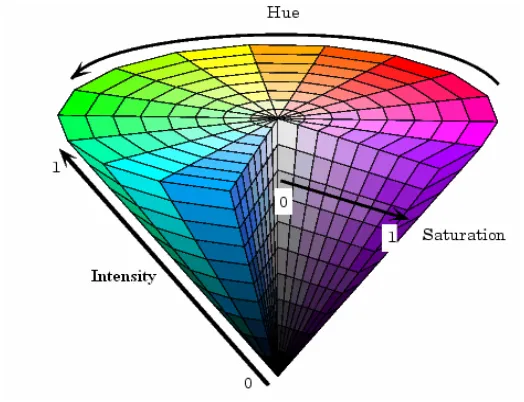
A special transformation map called (IHS), which stands for Intensity, Hue and Saturation can be obtained from the RGB bases, see figure 3.

Intensity is a measure of brightness:

I=(R+G+B)/3 (1)

Hue represents the color value:

H=cos-1{[(R-G) +(R-B)]/2[(R-G)2 +(R-B)(G-B)]-1/2} (2)

Saturation refers to the depth of the color:

(3)

123

Segmentation Methods in Face Recognition

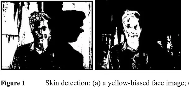
YCbCr is another transformation that belongs to the family of television transmission color spaces. Skin detection for face location in color images has benefited from these. R. Hsu et al. (2002) introduced a skin detection algorithm which starts with lighting compensation “reference white” which can be chosen from the top 5% of the luma if the sum of its pixels (>100). They detect faces based on the cluster in the (Cb/Y)-(Cr/Y) subspace. A sample of their result is shown next figure 1.

T. Chang et al. (1994) followed the same approach, while H. Wang and S. Chang (1997) choose the following system to convert form (RGB) to (Y, Cb, Cr):

(4)

Figure 1 Skin detection: (a) a yellow-biased face image; (b) a lighting compensated image; (c) skin regions of (a) shown as pseudo-color; (d) skin regions of (b). (R. Hsu et al., 2002)

S. Sirohey and A. Rosenfeld (2001) describe a method for extracting the skin area from an image using normalized color information. The flesh region is extracted and its color distribution is compared with a manually cropped model. J. Wang and E. Sung (1999) obtained 90% of correct detection rate with an identical method.

(5)

125

Figure 2 Skin color segmentation in HS space. (K. Sobottka and I. Pitas, 1996)

(6)

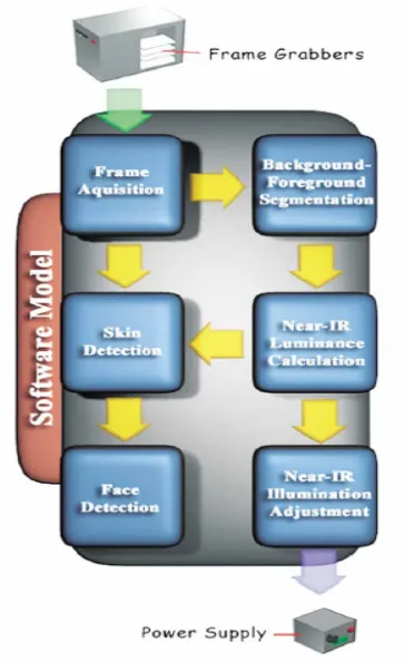
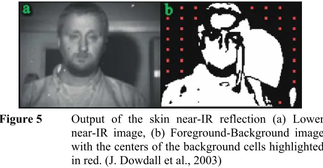
J. Dowdall et al. (2003) created a special hardware they call it Triple-band System where a Near-IR illumination generator is included figure 4. Their idea is centered in the fact that human skin has special reflection in the near-IR illumination. Next is an example of their output figure 5.

(7)

127

Figure 5 Output of the skin near-IR reflection (a) Lower near-IR image, (b) Foreground-Background image with the centers of the background cells highlighted in red. (J. Dowdall et al., 2003)

Whether using IHS or YCbCr transformation, the face region is checked to detect the elliptical shape. This method (color based) normally gives large false alarms, which require further processing either by considering other information or by calling other techniques for a relief, besides generating a skin color model is not a trivial task, for example M. Hu et al. (2004) used 43 million skin pixels from 900 images to train the skin-color model, B. Kwolek (2003) manually segmented a set of images containing skin regions for generating a skin model. It should be noticed too that RGB face databases are rare to be found and constructing them needs special expensive devices.

(8)

2.2 Based on Boundary

Frequently, an important visual element considered in image segmentation is the contrast between the face region and its background. The approaches for detecting such high contrast regions are called edge detection operators. From reviewing the literature it’s found that the most relied on operators are Sobel and Canny. The latter is proven to be the most efficient among all since it detects strong as weak edges and minimizes the noise, while it consumes more computational time than others do.

K. Kirchberg et al. (2002) calculate an edge magnitude image with the Sobel operator that uses the following mask:

∆x = [-1, 0, 1;-2, 0, 2;-1, 0, 1] Î Horizontal Magnitude Detection

∆y = [1, 2, 1; 0, 0, 0; -1, -2,-1] = [∆x]T Î Vertical Magnitude Detection

They created then a face model and superimposed it on a variety of discrete position and calculate the similarities using Hausdorff distance. F. Shih and C. Chuang (2004) adjust the edge generated image and use a raster scan from top to bottom and from left to right to yield the extreme points of the head whereby the bounding box can hug the whole face. A. Al-Qayedi and A.Clark (1999) use similar way however they have chosen SUSAN edge detector and they introduce an edge repairing method (for getting the chin segment). J. Wang and T. Tan (2000) use the Zero-crossing operator followed by an energy function to link cut edges.

M.Rizon and T. Kawaguchi (2000) examined the (x, y) location of each pixel of the Sobel edge, the head contour obtained by this method is not exact but they claimed that in all cases face features were present. S. Jeng et al. (1998) used a boost filtering window that combines a normalized Sobel filter coupled with normalized gray level; after this process is done they extract the edge and group blocks according to a predefined rule.

(9)

129

weigh coefficients. He initializes it on certain points of a previously Canny detected edge. “Snake” uses a controlled continuity spline function, transforming the shape of the curve to make the energy function minimized from the initial state of the curve (energy minimization). The final curve will end up hugging the shape of the object. The main difficulties of this method are the computational burden is so expensive, sensitivity to noise and hair; a good initial point is very hard to be estimated and the method will always converge onto a solution whether it is the desired one or false one. These methods under this section tend to work quite well for Binary images.

A. Somaie (1996) uses a specific 3*3 mask for edge detection to clip faces from the background, his mask operation on the image responds by a closed contour. The images were all shot in black background and a black cloth was draped around the subject’s neck. Therefore in his case, clipping such faces was not a trivial task. Rather it was one of the ancient direct techniques for face segmentation.

2.3 Based on Thresholding

(10)

1. Divide the original image into sub images and for each sub image do

2. Select an initial estimate for T

3. Segment the image using T. This will produce two groups of pixels. G1 consisting of all pixels with gray level values >T and G2 consisting of pixels with values <=T

4. Compute the average gray level values mean1 and mean2 for the pixels in regions G1 and G2

5. Compute a new threshold value

T = (1/2) (mean1 +mean2) (5)

6. Repeat steps 2 through 4 until difference in T in successive iterations is smaller than a predefined parameter T0

C. Lin and K. Fan (2000) use Thresholding method to generate 4-connected components. After labeling process, they get the center of mass of each block and find any three centers of three different blocks that form an isosceles triangle. They claim to have 98% correct detection rate on their set of database (500 images). L. Tao and H. Kwan (2002) use similar method to extract faces based on geometrical properties of faces features.

2.4 Based on Eigen faces

(11)

131

face candidates with a high fitness value are selected for further verification.

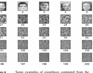
Turk and Pentland (1991) earlier developed this technique for face recognition. Their method exploits the distinct nature of the weights of eigenfaces in individual face representation. Since the face reconstruction by its principal components is an approximation, a residual error is defined in the algorithm as a preliminary measure of “faceness” This residual error which they termed “distance-from-face-space” (DFFS) gives a good indication of face existence through the observation of global minima in the distance map. Each PCA vector is called eigenvector, and when converted back to matrices these vectors can viewed as the eigenfaces of the dataset figure 6.

(12)

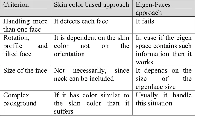
Eigenfaces and Color based approaches are among the most well known methods, and they are the state of the art in this field. Therefore, a comparison between the two is shown next (table 1).

Table 1 A comparison between Skin color and eigen based approaches

Criterion Skin color based approach Eigen-Faces approach Handling more

than one face

It detects each face It fails

Rotation,

profile and tilted face

It is dependent on the skin color not on the orientation

In case if the eigen space contains such information then it works

Size of the face Not necessarily, since

neck can be included It depends on the size of the eigenface size

Complex background

If it has color similar to the skin color than it suffers

Usually it handle this situation

2.5 Based on Neural Network

(13)

133

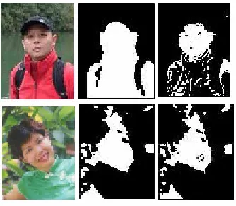
of non-skin data generated randomly from the In-house database. The networks trained on the In-house database were tested on all images in both the In-house and the WWW databases. The results are compared with a histogram-based skin detection system using the same databases Figure 7. The time taken for a neural network to be trained depends on the number of samples of the training data as well as on the number of neurons used.

Figure 7 Skin Detection on Sample Images from the WWW Database using Threshold Technique (Center) and Neural Network (Right). (J. Dargham et al., 2004)

(14)

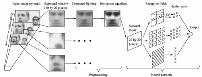
Figure 8 A face detection system using Neural Network proposed by H. Rowley et al. (1998)

Neural network method needs a lot of training samples in order to increase its efficiency level. The complexity of the network is considered to be its disadvantage because it cannot be known whether the network has “cheated” or not. It is almost impossible to find out how the network comes up with its answers. This is also known as a black box model.

2.5 Based on Genetic Algorithm (GA)

(15)

135

number of pixels in the actual ellipse. The ratio is large when both ellipses overlap perfectly.

K. Wong et al. (2001) use GA to select a pair of eyes among various possible blocks. The fitness value for each face candidate is calculated by projecting it onto the eigenfaces space. Even though GA is accurate, however like “snakes” it suffers from being a time consuming technique, because it will fire its chromosomes to all and every location.

2.6 Based on Voronoi Diagram

M. Suhail et al. (2002) explain how to extract some feature points from an image and then segment it based on these features. They determined a gradient magnitude which is larger than 75% to be extracted as point features from a window of size (3*3). Each of which forms the voronoi cell. These cells will generate the segmented image. In fact they use this method for non face images, however since the basic of it is the gradient magnitude, then it will not work properly for face segmentation. Besides determining the size of the window and the tolerance value of the accepted gradient is in itself a critical problem.

(16)

their paper. It is also sensitive to noise and beard. Their correct rate of detection of facial features upon segmentation is 89%.

Figure 9 An edge of the J-triangle splits the mergence of face skin and background (Y. Xiao and H. Yan, 2003)

3 FEATURES EXTRACTION

3.1 Chain Code

In practice, the best alternative, when exact representation is not possible, is to seek features allowing the original shape to be reconstructed to a reasonable degree of precision. This situation, which is opposite to the ideal exact representation, will be designated as an approximated representation. More formally, it can be said that a feature vector F provides an approximated representation of the shape S in case the respective reconstructed version:

) (

~ _T 1 _F

S = − G ₍₆₎

(17)

137

Segmentation Methods in Face Recognition ξ

≤ − =|| ~|| }

~ ,

{S S S S

Dist ₍₇₎

Where

ξ denotes a maximum allowed errors.

The Chain Code, Contour Code or Direction Code is a data structure to represent the boundary of a binary image on a discrete grid in an efficient way (B.Jähne,1997).

The algorithm is first coined by Freeman (H. Freeman, 1974). It encompasses a very compact representation since it is sufficient to use three bits to indicate which direction the next boundary is (M. Ren et al., 2002). It is a standard input format to many shape analysis algorithms because of its usefulness in detecting area, perimeter, moments, centers, eccentricity, projection and sharp turns (corners).

The starting point can be any point on the border of the object, however the often used way is to use an algorithm which scans the image line by line figure 10, thus the point will be the upper-most left pixel of the object. The boundary is followed in clockwise direction and the resultant code sequence is stored each time figure 11. If the object is not connected or has holes, then there will be a need to more than one chain code to represent it. When the pointer reaches to the first point, a normal practice is to delete the former coded edge pixels to allow for another tracing which takes the same steps unless the end of the array is reached. It is important to remember two pieces of information. First, the operation must remember the previous coded pixel for it will be used to eliminate the back-tracing to occur, which results normally with an infinite loop. Secondly, the (x,y) coordinates of the first tracked pixel for when it is revisited it will indicate that the contour is completely coded and thus the end of the operation on the object (G. Baxes, 1994).

(18)

code algorithm by introducing what is commonly known as Crack Code, they argued that is more precise, they claimed too getting an unbiased estimate of the area under straight line sections of a contour. However, they omitted analyzing their methods error rate due to sharp turns. Their method is characterised by using a point on the boundary between two pixels rather than the pixel centers (Chain Code) , the rest of the method is almost similar to Chain Code principal. This approach resulted in greater memory requirements, and somehow slower processing although having produced more accurate representation (G.Awcock and R.Thomas, 1996). Figure 12 visualizes the method. Another attempt to manipulate the Chain Code algorithm was done by (M.Ren et al., 2002), where they extracted the inner and outer contours of complex regions. Moreover, several generalizations have been made to make the Chain Code more efficient and accurate (R.Haralick and L. Shapiro, 1993), among which the Primitive Chain Code (PCC) which is discussed briefly in (M.Seul et al., 2000) but it is more complex to code and decode than Freeman Code. Contours are applicable for thin shapes not thick ones (L.Costa and R.Cesar, 2001). These coordinates are associated with rows and columns (matrix-like) and not with the traditional (x, y) Cartesian coordinates Figure 13.

(19)

139

Figure 11 Labeled neighborhood used by the contour tracking algorithms

(20)

Figure 13 The two pixel representations used for neighborhood tracking

Where

V0=(r, s+1), V1=(r-1, s+1), V2=(r-1, s), V3=(r-1, s-1), V4=(r, s-1), V5=(r+1, s-1), V6=(r+1, s) and V7=(r+1, s+1).

A contour traces a connected path between two pixels A and B which is a sequence of N pixels: P1,P2,….PN where each pair of consecutive pixels Pi,Pi+1 is such that Pi is a neighbor of Pi+1, with P1=A and PN=B. A connected component is a set of pixels such that there is a connected path between any pair of pixels in that set.

The inverse of a Chain Code is a geometric process and is given by:

The length of a Chain is given by:

(21)

141

Where

ne and n0 are the number of the even and odd-value links. The width and height of an enclosed contour is given by:

Width=maxj (Xj)- minj (Xj) (9) Height=maxj (Yj)- minj (Yj) (10)

Distance between two points is given by:

∑

= =

+ = n

i

n i ij ix a

a d

1 1

2 / 1 2

2 ₍ ₎ _]

) [(

(11)

In the array of Chain Code usually the following are recorded: E (1) Total number of all contour steps

E (2) X coordinate of the initial point E (3) Y coordinate of the initial point E (4) Label

E (5) Chain

Chain Code is said to be invariant to Translation. However, it is proved to suffer from the choice of starting point. To eliminate this sensitivity, the row code may be normalised (e.g.: Circularly rotating the raw code until the largest code value is leftmost). The chain code shows a number of obvious advantages over the matrix representation of a binary object.

Advantages:

• Compact Representation:

(22)

i.e.: about R2 pixels which need an R2 bit of storage. The bounding box is the smallest rectangle enclosing the object. However, if an 8 neighbor based chain code is used, the disk will be represented by far away less memory storage.

• Translation Invariance:

The Chain Code is translation invariant representaion of a binary object which makes the comaprision easier, and eliminated adding another algorithm to translate the object to the desired position.

• Fast Algorithm:

Since the Chain Code is a complete representation of an object or curve, any shape features can be computed, as well as the number of shape parameters (perimeter, area…etc), more efficiently using Chain Code representation than in the matrix representation.

• Voronoi Diagram:

A Voronoi Diagram (VD) is easily (with less computing time) constructed using Chain Code generated points.

• Moments Invariant can reduce their computation time by at least half if they were to use Chain Code representation intead of the real object.

Disadvantages:

• No Rotation Invariance:

(23)

143

Segmentation Methods in Face Recognition • No Scale Invariance

• Noise Sensitivity

Chain Code is sensitive to noise. Similar objects which have almost the same shape can have different Chain Code in presence of noise. Using black and white morphing and opening and closing operations can lessen down the noise and connect a broken Chains.

This method is used in some literature as a means to link edges of face contour to form a closed one, and that by examining the behaviour of the segments.

A. Kouzani et al. (1996) propose 8-neighboors based chain code to represent the edge of the features. The extracted string is then smoothed using a two step process to remove undesired symbols caused by noise, then the two adjacent inverse code are deleted and finally within a group of three or four codes having zero total vector rotation, each pair is replaced by a digit or a pair of digits based on its combination. As an example of the extracted features vectors the following:

Iris:

Pupil:

(24)

3.2 Template Matching

The simplest form of template matching is the comparison of the image of interest with a template image. A multiple templates can be used while searching for the closest one to its best fit feature. In here, lightening effects produce low fit even between images of same person. A deformable template was introduced, whereby a model of a face having its features (e.g.: eyes, nose…etc) linked with a spring-like was developed. This allowed a dynamic interaction with the image, which successfully eliminates the need for constructing multiple templates. However, the scale and rotation remain a problem. P. Hallinan et al.(1999) were accredited for introducing the deformable version of templates (elastic ones) .

Coorelation of a test pattern with a face template involves computing a measure of disparity between the face pattern and the test pattern. A threshold is set for the degree of disparity that can be associated with the given face (O.Ayinde and Y.Yang, 2002).

In their paper (J.Wang and T.Tan, 2000) used six templates. Two eyes templates and one mouth template were used to verify a face and locate its main features, then two cheek templates and one chin template were fired to extract the face contour. The performance claimed to be favorable except that it cannot detect faces with shadow, rotation and bed lighting conditions.

(25)

145

Going back to the deformable template, R.Chellappa et al.(1995) stated that when this kind of template started above the eyebrow, the algorithm failed to distinguish between the eye and the eyebrow. Another drawback to this approach is its computational complexity. In spite of these drawback points, some authors are in favor to it, because it is a logical way to be taken for feature extraction (R. Brunelli and T. Poggio, 1993).

3.3 Moments

Basically moments are designed to describe the properties of an object in terms of its area, position, orientation and other parameters. The basic equation of moment of an object is given as:

∑∑

= = − − = M x N y q S p S

pq B x y x x y y

1 1 ) ( ) )( , ( μ (12) Where

p,q is the order of the moment, (x,y) pixel coordinates and XS , YS represent the coordinates of the focal point.

Moment Centroid:

X’=m10/m00 (13)

and Y’=m01/m00 (X’, Y’) (14)

are the coordiantes of the centroid.

Moments are proven to be scale, translation and rotation invariant. Further details can be found in (M. Seul et al., 2000; G.Awcock and R.Thomas, 1996).

(26)

Moments invariants are among the statistical based approaches for features extraction, it has received a considerable attention in the recent years for its invariant properties. J. Haddadnia et al. (2002) use a modified version of moments called Pseudo Zernike Moment Invariant (PZMI) to generate a feature vector for each sub-image of the face possible features’ areas and fed these vectors to a classifier called Radial Basis Function (RBF) to determine a specific feature.

3.4 Color Based Algorithm

In here the deal is with non-binary images. Color is a good indicator for the presence of certain features, this fact led many researchers to look for clues to use color characteristics to extract features. In their paper (K. Sobottka and I. Pitas, 1996) noticed that in intensity images, eyes and mouth differ from the rest of the face because of their lower brightness. The reason for that is the color of the pupils, the sunken eye-sockets and the light red color of the lips. The rate of detection of facial features was 86%.

In their paper (K. Sobottka and I. Pitas, 1996) noticed that in intensity images, eyes and mouth differ from the rest of the face because of their lower brightness. The reason for that is the color of the pupils, the sunken eye-sockets and the light red color of the lips. The rate of detection of facial features was 86%.

In general, it is a representation of scenes with only two possible gray values for each pixel typically 0 and 1 contains object (foreground) and background, whether the object is represented by white or black pixels is just a matter of convention (L.Costa and R.Cesar, 2001) and chromaticity space, then the holes in the skin segmented image were thresholded to yield pixels of low intensity (e.g.: pupils,iris). The nostils however, were found by thresholding the normalized red component of the colors, finally for detecting the lips a thresholding was imposed again but this time on the normalized (Red+Blue-2*Green).

(27)

147

variations in static color images, based on lighting composition technique and non-linear color transformation. They extracted the eyes, mouth and face boundary based on their feature maps derived from both the luma and chroma of an image. They eye map is constructed by:

(15)

Where

C2b, (C~r)2, Cb/Cr are all normalized to the range [0,255], and the second parameter is denoted for the negative of Cr (e.g.: 255-Cr). By using morphological operations on the eye maps, eye candidates are brightened and other facial areas are suppressed Figure 14.

As for the mouth mapping, they based their algorithm on the observations that mouth region has stronger red component and weaker blue one than other features, therefore Cr>Cb, and the mouth has lower response in the Cr/Cb feature, but has a high response in C2r . Figure 15 shows the operation. Finally, for the face boundary map they used Hough Transformation.

(28)

Figure 15 Construction of the mouth maps for two subjects. (R. Hsu et al., 2002)

3.5 Morphological Operations

All morphological algorithms operate on binary images, which are the simplest, and yet one of the most useful image types. They are popular approaches where the operators work on the form of objects. In general, it is a representation of scenes with only two possible gray values for each pixel typically 0 and 1 contains object (foreground) and background, whether the object is represented by white or black pixels is just a matter of convention (L.Costa and R.Cesar, 2001). The convention of assigning 0 to background has a logical intuitive interpretation:

0 (“false”, “off”) Î Lack of object. 1 (“true”, “on”) Î Presence of object.

Assigning the 0 to background is a wise action because it saves ink.

Binary images can be a result of a direct acquisition or through application of specific image processing technique. They are important because shapes are herein understood as connected sets of points, help also for finding the center of mass, area, counting objects.

Erosion and Dilation

(29)

149

Erosion of set A by a structuring element B is defined as:

A Θ Bt ={P | Bp⊂A} (16)

Where

Bt is the transpose of B, and Bp is B centered at point p.

Erosion can enlarge holes in the object, shrink its boundary, eliminate ‘islands’ and remove narrow ‘peninsulas’ on the boundary (G.Awcock and R.Thomas, 1996).

Dilation is the ‘dual’ of erosion. It operates on the complement of set A namely A*, and it is defined as:

A Bt= A*ΘBt ={p | Bp ∩ A ≠Ø } (17)

Dilation fills in holes and expands the boundary of an object.

Closing and Opening

These are two operations based on the previous ones, and which are defined as follows:

‘Closing’ Î (dilate then erode) AB : (A Bt) ΘB (18) ‘Opening’ Î (erode then dilate) AB : (AΘBt) B (19)

The benefits of closing are that it blocks up small ‘lackes’ inside the object and links nearby objects. However opening may be used to eliminate small ‘islands’ and isolate objects which are just touching each other.

(30)

algorithm the reader is advice to pay a visit to their paper, however a show next a rough example figure 2.16.

Figure 16 The morphological operation process (a) The original image, (b) the profile signals of the dash line in (a), (c) the signals after performing the erosion operation, (d) the signals after performing the dilation operation, (e) the signals after performing the closing operation, and (f) the signals after performing the closing and clipped different operations. (C. Han et al., 2000)

3.6 Hough Transform

(31)

151

requirement, especially when the one knows the other name given to this method namely “Accumulator array” (M.Seul et al., 2000).

A well-known version of this is the Generalized Hough Transform (GHT), where the detected edge pixels vote for a shape according to a parametric representation or boundary orientation by referring to the centroid positions.

According to H. Moon et al. (2002) this method has a poor localization performance since it depends on the location of edges and points orientations, and it is hard to formulate the point spread function of the voting process. In addition, it is difficult to determine whether a peak is significant besides the size of the discrete parameter space increases rapidly as the number of parameters increases (B.Jähne,1997).

Another alteration for the Hough transform is found in the paper (A. Nikolaidis et al., 1997), where they used the Adaptive Hough Transform (AHT) to extract the cheeks and chin on a relevant sub image defined according to the ellipse containing the main connected component of the image, while they encountered problems in cheek extraction when the false symmetry of the ellipse leads to bad definition of the relevant sub image, and thus to an erroneous extraction of some other feature considered as predominant.

R. Chellappa et al. (1995) highlighted the fact that the application of Hough transform to detect the perimeter of the shape of the region below the eyebrows appears on average to yield a spacing 20% larger than the spacing between the irises.

3.7 Projection Function

(32)

S. Sirohey and A.Rosenfeld (2001) use the term “eyeness” to address the fact that human eye projection (mean value) has the “W” shape. They use this criterion to vote for eye-like region.

G. Feng and P. Yuen (1998) produced a system with a variance projection function that benefits from horizontal and vertical integral projections.

K. Sobottka and I. Pitas (1998) get the horizontal and vertical projections then the resulting reliefs are smoothed in x-direction by an average filter of width 3 and minima and maxima are determined. As a result, they obtain for each face candidate one smoothed y-relief with an attached list of its minima and maxima and, for each significant minima of the y-relief, smoothed x-reliefs with attached lists of their minima and maxima. By searching through the lists of minima and maxima, candidates of the three facial feature groups are determined. The groups and their characteristics as described next (table 2).

Table 2 Description of facial feature groups (K. Sobottka and I. Pitas, 1998)

Group 1: eyebrows,

eyes Group 2: nostrils Group 3: mouth, chin Two significant

minima

Upper/middle part of head

Significant maximum between minima Ratio of distance between minima to head width is in certain range Similar gray-levels

Two significant minima

Middle part of head Significant maximum between minima Small distance between minima Two significant maxima Middle/lower part of head Significant minimum between maxima

(33)

153

REFERENCES

A. Al-Qayedi and A. Clark, (1999). An Algorithm for Face and Facial-Feature Location Based on Grey-Scale Information and Facial Geometry. IEEE, 7th Int. Conf on Image Processing and its Applications, pp. 625-629.

A. Kouzani, F. He and K. Sammut, (1996). Constructing a Fuzzy Grammar for Syntactic Face Detection. Systems, Man, and Cybernetics, IEEE International Conference on, Volume: 2, 14-17 Oct.1996 pp: 1156 – 1161

A. Nikolaidis, C. Kotropoulos and I. Pitas, (1997). Facial Feature Extraction using Adaptive Hough Transform, Template Matching and Active contour Models. IEEE, 13th Int. Conf on Digital Signal Processing, pp. 865-868.

A. Okabe, B. Boots and K. Sugihara, (2000). Spatial Tessellations-Concepts and Applications of Voronoi Diagrams. Second Edition, Chichester: Wiley Series in probability and statistics.A.Paterson, (1991). Computerised Facial Construction and Reconstruction. No. 18: .Police technology : Asia Pacific police technology conference : proceedings of a conference. 12-14 November 1991. Australia. pp 136-144

A. Somaie, (1996). Face Identification using Computer Vision. University of Bradford USA: Ph.D. Thesis.

A. Trigui (2002). Voronoi Diagram and Delaunay Triangulations. Department Simulation of large Systems (SGS) Institute of Parallel and distributed Systems (IPVS) University of Stuttgart: Seminar

A. Yuille, P. Hallinan, and D. Cohen, (1992). Feature extraction from faces using deformable templates. Inernational Journal of Computer Vision 8, 99–111.

(34)

B. Kwolek. (2003). Face Tracking System Based on Color, Stereovision and Elliptical Shape Features. Proc, IEEE Inter Conf on Advanced Video and Signal Based Surveillance (AVSS’03) BioID, 2003. The BioID Face Database.

C. Han, H. Liao, G. Yu and L. Chen, (2000). Fast Face Detection via Morphology-Based Pre-Processing. Pattern Recognition 33 (2000) 1701-1712

C. Lin and K. Fan. (2000).Human Face Detection Using Geometric Triangle Relationship. IEEE Pattern Recognition Proceedings. Volume: 2 Pages:941 - 944 vol.2

D. Chadwick, (1991). Computer Identification System (CIDS): History, Synopsis and Future Directions. No. 18: Police technology : Asia Pacific police technology conference : proceedings of a conference. 12-14 November 1991. Australia. pp 114-116

D. Voth, 2003. Face Recognition Technology. IEEE Intelligent Systems Magazine, p 4-7

E. Hjelmas, B. Low, (2001). Face detection: a survey. Computer Vision and Image Understanding. 83 (2001) 236–274. E. Saber and E. Tekalp, (1998). Frontal-view face detection and facial feature extraction using color, shape and symmetry based cost functions. Pattern Recognition Letters 19 (1998) 669–680

F. Shih and C. Chuang, (2004). Automatic extraction of head and face boundaries and facial features. Information Sciences 158 (2004) 117–130

G. Awcock and R.Thomas, (1996). Applied Image Processing. USA: McGraw-Hill, Inc.

G. Baxes, (1994). Digital Image Processing. Canada: John Wiley and Sons.

G. Feng and P. Yuen, (1998). Variance projection function and its application to eye detection for human face recognition. Pattern Recognition Letters 19 (1998) 899–906

(35)

155

G. Gordan, (1992). Face Recognition Based on Depth and Curvature Features. IEEE Computer Society Conference on Computer Vision and Pattern recognition, pp. 808- 810. G. Khuwaja, (2002). An Adaptive Combined Classifier System for

Invariant Face Recognition. Elsevier Science Digital Signal Processing, 12: 21–46.

G. Reinelt, (1994). The Traveling Salesman. Germany: Springer-Verlag Berlin Heidelberg LNCS 840, pp. 42-63, 1994. G. Wang, Z. Houkes, B. Zheng and Y.Han, (1997). A New Method

for Fast Computation of Moments Based on 8-neighbor Chain Code Applied to 2-D Object Recognition. IEEE Int, Conference on Intelligent Processing Systems, pp.974-978. G. Yen and N. Nithianandan, (2002). Facial Feature Extraction

using Genetic Algorithm. Proceedings of the IEEE 2002 Congress on Evolutionary Computation, 2: 1895-1900. H. Dang and D. Claussi, (2004). Unsupervised image segmentation

using a simple MRF model with a new implementation scheme. Pattern Recognition 37 (2004) 2323 – 2335

H. Freeman, (1974). Computer processing of line-drawing images, ACM Computing Surveys. 6(1): 58-97.

H. Moon, R. Chellappa and A. Rosenfeld, (2002). Optimal Edge-Based Shape Detection. IEEE Transaction on Image Processing.11(11): 1209-1226.

H. Rowley, S. Baluja, and T. Kanade, (1998). Neural network based face detection. IEEE Transactions on Pattern Analysis and Machine Intelligence, 20(1):23–38

J. Dargham, A. Chekima and P. Pandiyan, (2004). Skin Detection using Neural Networks. Proceedings of the Second International Conference on Artificial Intelligence in Engineering & Technology. August 3-5 2004, Kota Kinabalu, Sabah, Malaysia. pp 371-376

J. Dowdall, I. Pavlidis and G.Bebis, (2003). Face Detection in the Near-IR Spectrum. Image and Vision Computing. 21: pp 565-578

(36)

Orders Pseudo Zernike Moment Invariant. Proc. Fifth IEEE Int, Conf on Automatic Face and Gesture Recognition. pp 315-320.

J. Wang and E. Sung, (1999). Frontal-view face detection and facial feature extraction using color and morphological operations. Pattern Recognition Letters 20 (1999) 1053-1068

J. Wang and T. Tan, (2000). A New Face Detection Method Based on Shape Information. Elsevier Science Pattern Recognition Letters. 21(2000): 463-471.

K. Bowyer, 2004. Face Recognition Technology: Security Versus Privacy. IEEE Technology and Society Magazine. Spring 2004 pp 9-20

K. Dunkelberger and O. Mitchell, (1985). Contour Tracing for Precision Measurement. Proc.IEEE Int, Conf on Robotics and Automation, pp.22-27

K. Kirchberg , O. Jesorsky, , R. Frischholz, (2002). Genetic Model Optimization for Hausdorff Distance-Based Face Localization. Proc. Inter, ECCV 2002 Workshop on Biometric Authentication, Springer, Lecture Notes in Computer Science, LNCS-2359, pp. 103-111, Copenhagen, Denmark

K. Sobottka and I. Pitas, (1996). Extraction of Facial Regions and Features Using Color and Shape Information. Proc. Int IEEE Conf on Image Processing, pp. 483-486.

K. Wong, K. Lam and W. Siu, (2001). An efficient algorithm for human face detection and facial feature extraction under different conditions. Pattern Recognition 34 (2001) 1993-2004

L. Costa and R.Cesar, (2001). Shape Analysis and Classification. USA: CRC Press.

(37)

157

M. Burge and W. Burger, (2000). Ear Biometrics in Computer Vision. Pattern Recognition Proceedings 15th International Conference on, Volume: 2, 3-7 Pages: 822 – 826

M. Ren, J. Yang and H. Sun, (2002). Tracing boundary contours in a Binary Image. Elsevier Science B.V Image and Vision Computing, pp.125-131.

M. Rizon and T. Kawaguchi, (2000). Automatic Eye Detection Using Intensity and Edge Information. TENCON2000. Proceedings, Volume: 2, Pages: 415 - 420 vol. 2

M. Seul, L. O’Gorman and M. Sammon, (2000). Practical Algorithms for Image Processing. USA: Cambridge University Press.

M. Suhail, M. Obaidat, S. Ipson and B. Sadoun, (2002). Content– Based Image Segmentation. Int IEEE Conference on SMC M. Turk and A. Pentland, (1991). Face Recognition Using Eigenfaces. Proc. CVPR, pp. 586-591

N. Ahuja.(1982). Dot Pattern Processing Using voronoi Neighborhoods. IEEE Trans on Pattern Recognition and Machine Intelligence. PAMI-4.3. 336-343

O. Ayinde and Y. Yang, (2002). Region-based Face Detection. Elsevier Science Pattern Recognition. 35(2002): 2095-2107.

P. Hallinan, G. Gordon, A. Yuille, P. Giblin and D. Mumford, (1999). Two-and Three-Dimensional Pattern of the Face. USA: A.K Peters, ltd.

R. Brunelli and T. Poggio, (1993). Face Recognition: Features Versus Templates. IEEE Transactions on Pattern Analysis and Machine Intelligence. 15(10): 1042-1052.

R. Chellappa, C. Wilson and S. Sirohey, (1995).Human and Machine Recognition of Faces: A Survey. Proc IEEE. 83 (5): 705-740.

R. Haralick and L. Shapiro, (1993). Computer and Robot Vision. USA: Addison-Wesley Publishing Company, Inc.

(38)

S. Jeng, H.Yuan, M. Liao, C. Han, M. Chern and Y.Liu, (1998). Facial feature detection using geometrical face model: an efficient approach. Pattern Recognition 31 (3) 273-282. S. Sirohey and A. Rosenfeld, (2001). Eye Detection in a Face

Image Using Linear and Non-Linear Filters. Pattern Recognition 34 (2001) 1367- 1391

T. Chang, T. Huang and C. Novak. (1994). Facial Feature Extraction from Color Images. IEEE 12th IAPR Int. Conf on Computer Vision and Image Processing, pp.39-43. T. Kanade, (1973). Picture Processing by Computer Complex and

Recognition of Human Faces. tech. rep., Tyoto Univ., Dept. of Information Science

V. Perlibakas, (2003). Automatical detection of face features and exact face contour. Pattern Recognition Letters 24 (2003) 2977–2985

Y. Xiao and H. Yan, (2002) Facial Feature Location with Delaunay Triangulation/Voronoi Diagram Calculation. Australian Computer Society, Inc. The Pan-Sydney Area Workshop on Visual Information Processing (VIP2001). Z. Tu and S. Zhu, (2002). Image Segmentation by Data-Driven

Markov Chain Monte Carlo. IEEE Transactions on Pattern Analysis and Machine Intelligence. Vol.24 No.5 May 2002, pp 657-673