Underdetermined Systems
Thesis by
Piya Pal
In Partial Fulfillment of the Requirements for the Degree of
Doctor of Philosophy
California Institute of Technology Pasadena, California
2013
c 2013
Acknowledgments
My years as a graduate student at Caltech have been one of the most defining phases of my life, one in which I grew both professionally and as an individual. As I fondly reflect back upon these years, I would like to thank many who have contributed in more than one way to this journey.
I have been most fortunate to have Prof. P. P. Vaidyanathan as my adviser. I am deeply indebted to him for giving me the freedom to pursue my ideas in research and providing unconditional support at every stage. He has inspired me to put utmost emphasis on creativity and originality, even if it requires one to boldly challenge decade-old established ideas. He has encouraged me to blaze new trails, rather than to follow an established one; to keep persevering even when the initial outcomes look disappointing; to be my own harshest critic so that I “bend over my back” to point out any potential drawback of my work; and above all, to enjoy this process every single day of my life. His life is an embodiment of work ethics and I have learned a lot by merely observing him on a daily basis. Finally, it is a pleasant coincidence that we share the same initials (P. P.) and it serves as a constant reminder of the great responsibility that comes with it.
on various topics ranging from academics to life in general. I would also like to express my deepest gratitude to Shuki, who has been a source of great support and inspiration, ever since my very first year at Caltech.
I would like to gratefully acknowledge the support of the Office of Naval Research (ONR) and Caltech which made this work possible.
Throughout my graduate years at Caltech, I have immensely benefited from interactions with some of the brightest minds. My special thanks extend out to the past and present members of my group, including Prof. Byung-Jun Yoon, Dr. Chun-Yang Chen (Scott), Dr. Ching-Chih Weng (Brian), Dr. Chih-Hao Liu (John), and Srikanth Tenneti. I learned a lot about life as a Ph. D student by observing Scott and Brian during my formative years. Although Byung-Jun had already left the group by the time I joined, he was always there when I needed him and provided generous advice regarding my career path. John has been my office mate and a dear friend for almost 5 years - we have shared some great times together, including conference trips to Paris and Prague, as well as our annual drive to Asilomar.
As I leave Caltech for the next phase of my career, I will be carrying fond memories of wonder-ful moments spent with some of the greatest friends I have. I would like to thank Teja, Rangoli, Prakhar, Nakul, JK, Sushree, Srivatsan, Vikas, Abhishek Saha, Kaushik Sengupta, Wei Mao, Na Li, Elizabeth and Zhiying for their friendship and company. I would also like to thank my friends among the staff in various offices in Caltech. I am thankful to Andrea Boyle, Caroline Murphy, Tanya Owen, and Lucinda Acosta for the care and promptness with which they took care of ad-ministrative matters. The international Students Program (ISP) Office at Caltech has always been a special place for me. It was at ISP where I met with many of my friends for the first time and I have always enjoyed being associated with ISP ever since. My special thanks to Laura Flower Kim and Daniel Yoder for their support and friendship. Laura has been a dear friend and I am going to treasure my many conversations with her. I would also like to express my sincere gratitude to Dr. Felicia Hunt - I cannot thank her enough for being a constant source of support and encouragement during my years at Caltech. The Caltech Glee Club has been an integral part of my life which I am going to dearly miss. I would like to thank our wonderful instructor Nancy Sulahian as well as dear friends Soyoung Park and Tiffany Kim for the great time we spend together on Monday and Wednesday evenings.
contributed towards making me what I am today. Without their unconditional love and many
sacrifices, I would not have come this far. My dad has always inspired me to boldly take up
chal-lenges in life and not be deterred by them, leading largely by his own example. I owe my love for literature, art and music to my mom, who is a voracious reader with razor sharp memory. My
brother, Subhabrata Pal, inspite of being a couple of years younger to me, has always acted like the
Abstract
A central objective in signal processing is to infer meaningful information from a set of measure-ments or data. While most signal models have an overdetermined structure (the number of un-knowns less than the number of equations), traditionally very few statistical estimation problems have considered a data model which is underdetermined (number of unknowns more than the number of equations). However, in recent times, an explosion of theoretical and computational methods have been developed primarily to study underdetermined systems by imposing sparsity on the unknown variables. This is motivated by the observation that inspite of the huge volume of data that arises in sensor networks, genomics, imaging, particle physics, web search etc., their information content is often much smaller compared to the number of raw measurements. This has given rise to the possibility of reducing the number of measurements by down sampling the data, which automatically gives rise to underdetermined systems.
In this thesis, we provide new directions for estimation in an underdetermined system, both for a class of parameter estimation problems and also for the problem of sparse recovery in compres-sive sensing. There are two main contributions of the thesis: design of new sampling and statistical estimation algorithms for array processing, and development of improved guarantees for sparse reconstruction by introducing a statistical framework to the recovery problem.
We consider underdetermined observation models in array processing where the number of un-known sources simultaneously received by the array can be considerably larger than the number of physical sensors. We study new sparse spatial sampling schemes (array geometries) as well as propose new recovery algorithms that can exploit priors on the unknown signals and unambigu-ously identify all the sources. The proposed sampling structure is generic enough to be extended to multiple dimensions as well as to exploit different kinds of priors in the model such as correlation, higher order moments, etc.
Contents
Acknowledgments iv
Abstract vii
1 Introduction 1
1.1 Estimation in Array Processing . . . 2
1.1.1 Signal Model and Role of Autocorrelation . . . 2
1.1.1.1 The Array Signal Model . . . 3
1.1.1.2 Autocorrelation and Spectral Estimation . . . 5
1.1.2 Parametric Estimation . . . 6
1.1.3 Spectral Estimation . . . 7
1.1.4 Sampling and Underdetermined Estimation . . . 8
1.1.5 New Questions in Array processing . . . 9
1.2 Sparse Estimation and Compressive Sensing . . . 11
1.2.1 The Ubiquitous Sparse Model . . . 11
1.2.2 A Brief Review of Sparse Estimation . . . 12
1.2.2.1 A Brief History of Sparse Recovery Algorithms . . . 12
1.2.2.2 Extensions . . . 14
1.2.3 New Questions in Sparse Estimation . . . 15
1.3 Outline and Scope of the Thesis . . . 16
1.3.1 Nested Arrays in One Dimension (Chapter 2) . . . 16
1.3.2 Nested Arrays in Two Dimensions (Chapter 3) . . . 17
1.3.3 Higher Order Statistics and Extension of Nested Arrays (Chapter 4) . . . 17
1.3.4 Wideband Beamforming and Estimation (Chapter 5) . . . 18
1.3.6 Correlation Aware Sparse Recovery (Chapters 7 and 8) . . . 19
1.4 Notations . . . 20
2 Nested Arrays in One Dimension 21 2.1 Introduction . . . 21
2.2 Outline . . . 24
2.3 Definitions and Signal Model based on Difference Co-array . . . 24
2.4 The Co-Array Perspective . . . 25
2.4.1 Properties of Difference Co-Array: . . . 26
2.4.2 Computing the Weight Function: . . . 28
2.4.3 Comparison of underdetermined DOA estimation techniques from the co-array perspective . . . 28
2.5 The Concept of Nested Array: Degrees of Freedom and Optimization . . . 29
2.5.1 Two Level Nested Passive Array. . . 30
2.5.2 K Levels of Nesting . . . 32
2.5.3 Optimization of the K level nested Array . . . 33
2.5.4 Remarks . . . 34
2.6 Applications of the nested Array in DOA estimation of more sources than Sensors . 35 2.6.1 Spatial Smoothing based DOA estimation: . . . 36
2.6.2 Remarks: . . . 39
2.7 Beamforming with increased Degrees of freedom . . . 40
2.7.1 Deterministic Beamforming . . . 41
2.7.2 Nulling of Jammers and Noise. . . 41
2.7.3 MVDR-like Beamforming . . . 42
2.8 Numerical Examples . . . 43
2.8.1 MUSIC spectra . . . 43
2.8.2 RMSE v/s SNR and snapshots . . . 44
2.8.3 Detection Performance . . . 46
2.8.4 Resolution Performance . . . 46
2.8.5 2 level vs optimally nested array. . . 48
2.8.6 Beamforming . . . 48
2.8.6.2 Jammer and noise Nulling . . . 49
2.8.6.3 MVDR-like Beampattern . . . 51
2.9 Conclusion . . . 52
2.10 Appendix . . . 52
2.11 Proof of Theorem 2.5.1 . . . 52
3 Nested Arrays in Two Dimensions 54 3.1 Introduction . . . 54
3.2 Outline . . . 55
3.3 Review and Definitions of Multidimensional lattices and Integer Matrices . . . 56
3.4 Revisiting Difference Co-Arrays . . . 58
3.5 Nesting of Arrays on Lattices . . . 60
3.5.1 Properties of the Nested Array . . . 61
3.5.2 A Specific Construction . . . 62
3.6 Orientation Issues of the Two Dimensional Nested Co-Array . . . 64
3.6.1 Sensor Configuration I: . . . 65
3.6.1.1 Sensor Locations . . . 65
3.6.1.2 Positive and Negative Halves of the difference co-array . . . 66
3.6.2 Sensor Configuration II: . . . 67
3.6.3 Configuration on Offset-Lattice . . . 68
3.7 A Smith-Form Perspective to 2D Nested Array . . . 70
3.7.1 Smith Form of the integer matrixP . . . 71
3.7.2 Co-array design in Smith domain . . . 73
3.7.2.1 Smith form Based Design using Offset Configuration . . . 74
3.7.2.2 Smith Form Based Design Using Configuration II . . . 74
3.7.3 Inclusion of the0element . . . 78
3.8 Optimization of Degrees of Freedom . . . 79
3.8.1 Maximization of degrees of freedom in the offset configuration . . . 79
3.8.2 Maximization of the degrees of freedom in Configuration II . . . 80
3.8.3 Optimal Solution with1DUniform Linear Arrays . . . 83
3.9.1 Signal Model Based on the difference co-array: . . . 85
3.9.2 Invariance in the Difference Co-Array . . . 88
3.9.3 Novel Rank Enhancing Algorithm for DOA Estimation . . . 89
3.10 Identifiability Issues . . . 91
3.10.1 Rank of the Array Manifold matrix in2D . . . 92
3.10.1.1 Sufficient Condition for full column rank ofA0,0forD≤M N . . 94
3.10.1.2 Column Rank Deficiency of the array manifoldA0,0whenD≤M N 95 3.10.2 A Sufficient Condition on Unique Identifiability . . . 97
3.10.2.1 Example (Full column rank ofA0,0does not imply unique identi-fiability) . . . 97
3.11 Simulations . . . 99
3.11.1 MUSIC spectra . . . 99
3.11.2 RMSE v/s SNR and snapshots . . . 100
3.11.3 Detection Performance . . . 101
3.12 Conclusion . . . 101
3.13 Appendix . . . 103
3.13.1 Proof of Theorem 3.7.2 . . . 103
3.13.2 Proof of Theorem 3.8.1 whenKis odd . . . 105
3.13.2.1 K+ 1 = 4p+ 2 . . . 106
3.13.2.2 K+ 1 = 4p . . . 106
3.13.3 Proof of Theorem 3.8.2 . . . 108
4 Higher Order Statistics and Extension of Nested Arrays 110 4.1 Introduction . . . 110
4.2 Outline . . . 112
4.3 Review of2qth order cumulants and their role in array processing . . . 112
4.3.1 Data Model . . . 113
4.3.2 2qth order circular cumulants . . . 113
4.3.3 Virtual Array Associated with2qth Order cumulants . . . 115
4.4 A New Look into the Virtual Array Associated with2qth order Cumulants . . . 116
4.4.1 Higher Order Difference Co-Array . . . 117
4.4.3 Independence from Orientations . . . 120
4.5 Nested Array with2qlevels and its virtual array . . . 122
4.5.1 Bonus ULA segment . . . 123
4.5.2 Comments on the main and bonus ULA segments . . . 124
4.6 Optimization of the number of virtual sensors . . . 124
4.6.1 Optimal Sensor Allocation Problem (without the extra segment) . . . 125
4.6.2 Relation to exponential array . . . 127
4.6.3 Optimization including the extra ULA segment . . . 127
4.7 Underdetermined DOA estimation with2qlevel Nested Array . . . 128
4.7.1 Proposed Spatial Smoothing Based Algorithm . . . 129
4.7.2 Comparison with2qMUSIC . . . 131
4.8 Comments on Identifiability and Cramer Rao Bound . . . 132
4.8.1 Identifiability . . . 132
4.8.2 An Upper Bound on Identifiability . . . 133
4.8.3 Achieving the Upper Bound with the Proposed Method . . . 134
4.8.4 Cramer Rao Bound Study . . . 135
4.8.4.1 Deterministic Cramer Rao Bound . . . 135
4.8.4.2 Stohcastic Cramer Rao Bound . . . 136
4.9 Simulations . . . 137
4.9.1 Representative MUSIC Spectra . . . 138
4.9.2 RMSE vs Snapshots . . . 138
4.9.3 RMSE vs SNR . . . 139
4.9.4 Model Perturbation . . . 139
4.9.5 Probability of Resolution . . . 141
4.10 Conclusion . . . 142
4.11 Appendix . . . 143
4.11.1 Virtual Sensors in the2qth order Difference set . . . 143
4.11.1.1 Proof of Theorem 4.5.1 . . . 143
4.11.1.2 Virtual sensors in the extra ULA segment . . . 145
5.2 Outline . . . 153
5.3 Background of Wideband Beamforming . . . 153
5.3.1 Signal Model . . . 153
5.3.2 Review of Coherent and Incoherent Methods of Wideband DOA Estimation . 155 5.4 Autofocusing approach to coherent signal subspace based wideband DOA estimation 157 5.5 Simulation Examples . . . 162
5.6 Introduction to Frequency Invariant Beamforming . . . 164
5.7 Theory of Lattice Based Frequency Invariant Beamforming without Filters . . . 165
5.7.1 Realization of Lattice Based Frequency Invariant Beams . . . 167
5.7.2 The Beampattern in the Transform domain: Variation of Contours with lattices 169 5.7.2.1 Constant spatial direction (θ) contours: . . . 169
5.7.2.2 Constant temporal frequency (ω) contours: . . . 169
5.7.2.3 Effect of angle between lattice generator vectors on the beampattern 170 5.7.3 Realization Issues: Rectangular v/s Circular Sampling . . . 173
5.7.4 Examples . . . 175
5.7.5 RMSE of approximation . . . 175
5.8 Efficient Realization of the lattice based frequency invariant beamforming using Vir-tual Array . . . 178
5.8.1 Wideband Beamforming Based on Difference Co-array . . . 179
5.8.2 Realization of the lattice as the difference co-array . . . 182
5.8.3 Frequency Invariant Beamforming using the difference array: . . . 183
5.8.4 Examples . . . 185
5.9 Concluding Remarks . . . 187
6 Coprime Sampling Arrays and Commuting Coprime Matrices 188 6.1 Introduction . . . 188
6.1.1 Preliminaries . . . 189
6.1.2 Chapter outline . . . 192
6.2 Circulant matrices . . . 192
6.2.1 Relation to DFT . . . 194
6.2.2 Embedding circulants into unimodular matrices . . . 196
6.3 Skew Circulants . . . 198
6.3.1 Derivation of the conditions for coprimality . . . 198
6.3.2 Coprimality of determinants . . . 202
6.3.3 Adjugate pairs . . . 202
6.3.4 Comparing with circulants . . . 203
6.4 Triangular matrices . . . 204
6.4.1 Remarks . . . 205
6.4.1.1 Adjugate pairs . . . 205
6.4.1.2 Right coprimality . . . 206
6.4.1.3 Commuting triangles . . . 206
6.5 Other related matrices . . . 206
6.5.1 Reflected triangles . . . 207
6.5.2 General matrices with three freedoms . . . 208
6.5.3 Testing coprimality by triangularization . . . 208
6.5.4 Unimodular similarity transforms . . . 209
6.6 3×3Triangular matrix and adjugate . . . 210
6.7 Concluding remarks . . . 211
7 A Correlation Aware Framework For Sparse Estimation: Ideal Covariance Matrix 213 7.1 Introduction and Related Work . . . 213
7.2 Related Work . . . 214
7.3 Review of Conditions for Uniqueness of Sparse Representations . . . 216
7.4 Our Contributions . . . 218
7.4.1 A Correlation Aware Framework . . . 218
7.4.2 Recovery of Sparse Support v/s Sparse Vector . . . 219
7.5 Uniqueness of Support Recovery From Exact Data Covariance . . . 220
7.5.1 Deterministic Designs: Revisiting Nested Arrays . . . 225
7.6 Convex Relaxation for Support Recovery from Ideal Covariance Matrix . . . 228
7.6.1 New Coherence Based Guarantee . . . 228
7.7 The case of Positive Solution . . . 230
7.7.1 Conditions for Perfect recovery of non negative solution . . . 230
7.7.3 Simulations . . . 232
7.8 Orthogonal Matching Pursuit on the Covariance Matrix . . . 235
7.8.1 The Exact Reconstruction Condition for OMP . . . 235
7.8.2 Guarantees for the Co-SMV Model . . . 236
7.9 Conclusion . . . 237
8 Estimated Covariance matrix and the Multiple Measurement Vector Model 239 8.1 Introduction . . . 239
8.1.1 Related Work and Our Contributions . . . 240
8.2 Outline of Chapter . . . 241
8.3 MMV Model and the Estimated Correlation Correlation . . . 241
8.4 Fundamental Conditions for Sparse Support Recovery Under Bounded Noise . . . . 243
8.5 Analysis of LASSO: Independent of Distribution . . . 247
8.6 Analysis of LASSO For Gaussian Model . . . 249
8.6.1 Concentration Inequalities . . . 250
8.6.2 Probability of Support recovery by Solving the LASSO . . . 251
8.7 Numerical Results . . . 252
8.8 Conclusion . . . 254
8.9 Appendix . . . 255
8.9.1 Proof of Theorem 8.5.1 . . . 255
8.9.2 Proof of Theorem 8.6.2 . . . 257
8.9.3 Proof of Lemma 8.6.3 . . . 258
8.9.4 Proof of Lemma 8.5.1 . . . 259
9 Future Directions 262
List of Figures
1.1 Figure showing plane wave propagating along the directionv(θ, φ)and received by an array of sensors. Hereθdenotes the elevation andφdenotes the azimuthal angle. . 3 2.1 A2level nested array with3sensors in each level (top), and the weight function of its
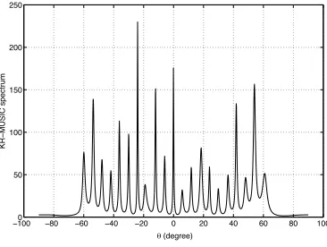
difference co-array (bottom). . . 31 2.2 Theith nesting level containingNisensors in aK-level nested linear array. . . 32 2.3 MUSIC spectrum using the SS-method and the QS-method, as a function of sine of the
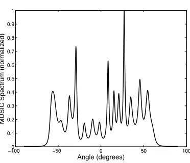
DOA,N = 6,D= 8,T = 4800, SNR= 0dB. . . 44 2.4 MUSIC spectrum using the SS-method and QS-method, as a function of sine of the
DOA. HereN = 6,D= 8,T= 480, SNR= 0dB. . . 44 2.5 RMSE (in degrees) vs. SNR (for the source at30◦) of QS and SS methods applied on2
level nested array and ordinary MUSIC on a12element ULA, withT = 800,N= 6. . 45 2.6 RMSE (in degrees) vs. SNR (for the source at30◦) of QS and SS methods applied on2
level nested array and ordinary MUSIC on a12element ULA, withT = 4800,N = 6. 45 2.7 RMSE (in degrees) vs. the number of snapshotsT(for the source at30◦) of QS and SS
methods applied on2level nested array and ordinary MUSIC on a12element ULA. Here SNR= 6dB,N = 6. . . 46 2.8 Comparison of detection performance of SS method applied to2 level nested array
and MUSIC applied to12element ULA as a function of number of snapshots. Here SNR= 10dB,N = 6. . . 47 2.9 Comparison of resolution performance of SS-MUSIC method applied to2level nested
array with 6 sensors and traditional MUSIC applied to a12 element ULA and a6 element ULA, as a function of SNR for two closely spaced sources at12◦and14◦. . . . 47 2.10 MUSIC spectrum for QS-method applied to the optimally nested array withN = 6,
2.11 MUSIC spectrum for QS-method applied to the 2 level nested array with N = 6,
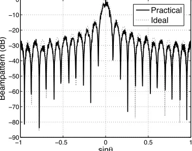
T = 16200,D= 27and SNR= 0dB. . . 49 2.12 Practical deterministic sinc beampattern obtained by non linear beamforming from
the2level nested array,N= 6,T = 100. . . 50 2.13 Signal-to-Jammer-and-noise-ratio (SJNR) vs number of snapshots (averaged over1000
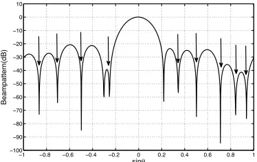
Montecarlo runs) for2level nested array with4sensors and the equivalent ULA with 11sensors, Number of jammers= 6, SNR= 0dB, SJR=−20dB. . . 51 2.14 Practical Beampattern obtained from the2level nested array after nulling6jammers
and noise,N = 4,T= 100. . . 51 2.15 Ideal MVDR-like beampattern obtained by applying spatial smoothing to the2level
nested array,N = 6, usingT = 1000snapshots for computing the smoothed covari-ance matrix. . . 52
3.1 Fundamental parallelepiped (FPD) of the lattice generated by the generator matrix
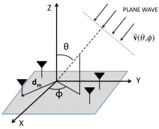
V= [v1 v2] . . . 57 3.2 FPDs of dense lattice generatorN(d)and sparse lattice generatorN(s), whereN(s) =
N(d)P. HereN(d)is randomly generated (with the shaded FPD) andPis as given in the text. Also shown are the sensors belonging to the sparse and dense lattices where
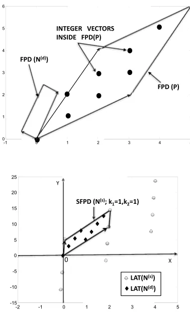
LAT(N(s))is included withinLAT(N(d)). . . 60 3.3 (top) The integer vectors inside F P D(P) (total number of such vectors is det(P))
which denote the locations of the sensors on the dense lattice generated byN(d)(here
N(d) is randomly generated andPis given in the text). Also shown isF P D(N(d)). (bottom) This choice of location of det(P)sensors on the dense latticeLAT(N(d)) com-pletely tilesSF P D(N(s), k
1, k2).In this example,k1= 1, k2= 1. . . 63 3.4 (left) A2D nested array with6sensors on the dense lattice and12sensors on the sparse
lattice, and (right) its corresponding difference co-array elements given byN(s)n(s)−
N(d)n(d). HereN(d)is randomly generated andPis given in the text. . . 64 3.5 (top) A2D nested array with sensor locations as given in Configuration I. (bottom)
3.7 (top) A2Dnested array with sensor locations as given in Configuration II. (bottom) Corresponding difference co-array, where the positive and negative halves form a con-tinuum and also their overlap is reduced to a line with only9sensors. . . 69 3.8 (top) A2Dnested array with sensor locations as given by Offset Configuration.
(bot-tom) Corresponding difference co-array, with no overlap. . . 70 3.9 The FPD ofN(s)andN(d)for the case wherePis a non-diagonal integer matrix. Their
geometries look very different. . . 71 3.10 FPDs ofN˜(s)andN˜(d)obtained by taking the Smith form ofP.The FPDs are scaled
versions of each other with each side ofF P D(N˜(s))being3times that ofF P D(N˜(d)) sinceΛ= 3I. . . 72 3.11 (Top) FPD ofN(d) and circles indicating the index setn(d)
c (Bottom) FPD of N˜(d) =
N(d)U
1and circles indicating the index set˜n
(d)
c =U1−1n
(d)
c which describe contigu-ous elements onLAT(N˜(d)). . . . 75 3.12 (Top)2DNested array designed in Smith domain showing the location of the sparse
and dense sensors onLAT(N˜(s))and LAT(N˜(d))respectively withΛ = 3I, N(s) 1 =
2, N2(s)= 3.There are(2N1(s)+ 1)N2(s)−1 = 14sensors on the sparse and det(Λ) = 9 sensors on the dense lattice. (Bottom) Corresponding difference co-array with2(2N1(s)+ 1)N2(s)λ1λ2−(2N
(s)
1 + 1)λ1= 255sensors onLAT(N˜(d)). . . 76 3.13 The co-array of the Offset Configuration without the physical element at position0,
resulting in holes. . . 78 3.14 An example of the optimal solution where the physical array is union of two1DULAs,
and the corresponding contiguous sensors on the difference co-array. HereK = 9, henceK1= 4,K2 = 5. The total number of contiguous virtual elements in the differ-ence co-array is(K+ 1)2/2−(K+ 1)/2 = 45. . . . 83 3.15 Subarrays of a2Darray with contiguous elements on a lattice. HereS0,0is the
3.16 The virtual difference co-array array of2Dnested array and its subarrays used for the proposed DOA estimation algorithm based on spatial smoothing. The virtual array is of sizeM×NwhereM = 17,N = 17. The fundamental subarray is of size(M+ 1)2× (N+ 1)/2 = 9×9and there are a total of(M + 1)(N + 1)/4 = 81subarrays, each of which is a shifted copy of the fundamental subarray. . . 90 3.17 M N = 30pairs of(ω1, ω2)obtained according to Lemma 3.10.1 by generatingM = 5
random values ofω1andN = 6random values ofω2. . . 95 3.18 2D MUSIC spectrum using the proposed algorithm for identifying D = 36 sources
using the2Dnested array for two values of snapshots. . . 100 3.19 Comparison of RMSE (in degrees, averaged over all D = 36DOA pairs) vs. SNR
between the proposed DOA estimation algorithm applied on the2D nested array, and traditional2DMUSIC applied on the benchmark array. HereT = 500. . . 100 3.20 Comparison of RMSE (in degrees, averaged over allD= 36DOA pairs) vs. the
num-ber of snapshots between the proposed DOA estimation algorithm applied on the 2D nested array, and traditional2D MUSIC applied on the benchmark array. Here SNR= 6dB. . . 101 3.21 Comparison of probability of detecting all theD= 36sources for the2Dnested array
and the benchmark array, as a function of the number of snapshots. Here SNR= 10dB. 102
4.1 An arbitrary physical array and its various higher order virtual arrays (top left) The physical array with3 arbitrarily generated sensor locations (top right) Virtual array (difference co-array) forl = 1, q = 2. (bottom left) Virtual array (sum co-array) for
l= 2, q= 2. (bottom right)2q= 4th order difference co-array. . . 121 4.2 Optimal4level nested array (optimized without considering the extra ULA segment)
with6sensors and its4th order difference co-array. Notice the extra ULA segments that extend out. . . 126 4.3 MUSIC Spectra for D = 8 sources, produced by (top left),(bottom left) Proposed
Method on a 4 level nested array with 6 sensors and (top right),(bottom right)2q
MUSIC on a ULA with6sensors. HereT = 800, for (top left) and (top right), and
4.4 MUSIC Spectra for D = 2 sources, produced by (top left),(bottom left) Proposed Method on a 4 level nested array with 6 sensors and (top right),(bottom right)2q
MUSIC on a ULA with6sensors. HereT = 2000, for (top left) and (top right), and
T = 5000for (bottom left) and (bottom right). SNR= 6dB. . . 140 4.5 RMSE vs number of snapshots (T) of the proposed method and4MUSIC
correspond-ing to (top)D= 6sources, and (bottom)D= 8sources. HereN = 6, SNR= 6dB. No Model Perturbation. . . 140 4.6 RMSE vs SNR (in dB) of the proposed method and4MUSIC corresponding to (top)
D = 6 sources, and (bottom)D = 8 sources. HereN = 6, T = 2000. No Model Perturbation. . . 141 4.7 RMSE vs number of snapshots (T) of the proposed method and4MUSIC for the
per-turbed model. HereN = 6, SNR= 6dB,D= 6. . . 142 4.8 Probability of resolving the two sources at30◦and 32◦ of the proposed method
ap-plied on4level nested array and4MUSIC on ULA. HereN = 6, SNR= 6dB. . . 142 5.1 Comparison of RMSE of the different wideband DOA estimation algorithms v/s SNR
for the source at45◦. . . 163 5.2 Comparison of Bias of the different wideband DOA estimation algorithms v/s SNR
for the source at45◦.. . . 163 5.3 MUSIC spectrum for the three sources at0◦,30◦and45◦using i) proposed
autofocus-ing approach (top) and ii) TOPS (bottom) at SNR=0 dB. . . 164 5.4 Constantθ(0≤θ≤180)contours in (ω1−ω2) plane for different values ofψ. . . 170 5.5 Constantω(π/2≤ω≤π) contours in (ω1−ω2) plane for different values ofψ. . . 170 5.6 Plot of the slopeφof the constantθcontours in the (ω1−ω2) plane vs the spatial angle
θfor different values of the lattice angleψ. . . 172 5.7 Proposed sampling in (ω1−ω2) plane forψ= 10◦. . . 174 5.8 Proposed sampling in (ω1−ω2) plane forψ= 90◦. . . 175 5.9 Frequency Invariant Beampattern as a function ofsinθfor50values ofω uniformly
betweenπ/2andπrealized using lattice withψ= 15◦,M =N = 17. . . . 176 5.10 2dimensional plot of realized frequency invariant beampattern, as a function of
spa-tial directionsinθand temporal frequencyω, realized using a lattice withψ= 15◦and
5.11 Frequency Invariant Beampattern as a function ofsinθfor50values ofω uniformly betweenπ/2andπrealized using lattice withψ= 90◦,M =N = 17. . . 177 5.12 2dimensional plot of realized frequency invariant beampattern, as a function of
spa-tial directionsinθand temporal frequencyω, realized using a lattice withψ= 90◦and
M =N = 17. . . 177 5.13 RMSE of realizing the frequency invariant beam v/s lattice angleψfor two arrays of
size9×9and17×17. . . 178 5.14 Two examples of1Darrays and their cross difference co-array on a2Dlattice. (a) and
(c) denote the physical arrays, (b) and (d) denote the corresponding cross difference co-arrays. . . 183 5.15 Difference co-array based frequency invariant beampattern as a function ofsinθusing
two 17 element ULAs plotted for three values of ω = π/2,3π/4 and π, using200 snapshots. . . 186 5.16 Evolution of jammer nulling with snapshots (T) based on the difference co-array using
two17element ULAs withψ= 45◦with jammer directions given by{60◦,45◦,30◦,15◦}.186 6.1 (a) A multidimensional decimator and expander in cascade. (b) System with
decima-tor and expander interchanged. . . 189 6.2 (a), (b) Two dimensional arrays with sensors on integer lattices, and (c) the coarray. . 190
7.1 Comparison of recovered DOAs by nested array and ULA for different values ofT
(top left) Reconstructed DOAs using nested array withD = 5,T = 200. (top right) Reconstructed DOAs using ULA withD = 5,T = 200. (bottom left) Reconstructed DOAs using ULA with D = 5,T = 800, and (bottom right) Reconstructed DOAs using nested array withD= 8,T = 400. . . 233 7.2 Comparison of resolution performance between nested array and ULA (top)
Recon-structed DOAs using nested array forD = 2,T = 200, and (bottom) Reconstructed DOAs using ULA forD= 2,T = 200. . . 234 8.1 Comparison of recovered support when| S0 |= 34 > M. (top left): True Support.
List of Tables
3.1 Summary of design of nested array in Smith domain. . . . 77 3.2 Solution to Problem (3.10) . . . 79 3.3 Solution to Problem (3.12) Using StrategyS∆ . . . 82 3.4 Solution to Problem (3.13) . . . 82
Chapter 1
Introduction
The theory of statistical estimation is concerned with extraction of meaningful information from available data or measurements. In recent times, there has been an exponential rate of increase in the amount of data that is available in almost every application area, leading to the so called “data deluge” [8]. The “Big Data” routinely arises in sensor networks, genomics, remote sensing, imag-ing, particle physics, web search, social networks, and so forth. This has led to a widening gap between the volume of available data and the capabilities for storing, communicating and process-ing them efficiently. Fortunately however, the amount of information buried in the data acquired by sensors in most scenarios is substantially lower compared to the number of raw samples acquired. This key observation has led to the possibility of sampling strategies and design of sensing systems that can directly capture the information using far fewer samples (typically achieved by random projections). In many natural scenarios, the physics of the problem itself imposes structures on the ensuing acquisition system, leading to the possibility of “structured sampling” strategies. Also of-ten, one can make informed assumptions about the nature of randomness, or statistical distribution of the data which can be possibly exploited to our advantage for extracting information. In fact, in many cases, one is actually interested in estimating parameters of the underlying distribution of the model from the statistics of the data.
complexity does not drastically scale with the volume of the data?
The work presented in this thesis addresses these questions by revisiting a much unexplored frontier of estimation theory, namely that of an underdetermined observation model. The first part of the thesis focuses on underdetermined signal models arising in antenna array processing. It is devoted to development of new theoretical guarantees and practical sampling and estimation schemes to attain those guarantees. In the second part, we consider underdetermined systems which exhibit sparsity and demonstrate that our approach can be generalized to this case as well, leading to a new theory of correlation aware sparse estimation.
In this introductory chapter, we review the history and developments of the problems of interest in this thesis: namely algorithms for antenna array processing, and the theory of sparse signal representation and estimation. Due to the large volume of existing literature, the summary here is only directly related to the current thesis and is by no means a complete treatment of all past work. Please refer to [186, 104, 96, 187, 24, 56] for a more comprehensive treatment.
1.1
Estimation in Array Processing
We present a broad review of estimation algorithms used in array processing. Many of these tech-niques apply to more general estimation problems beyond the particular application of sensor ar-rays. The space-time model of array processing also has a more general interpretation which will be revisited in the context of sparse estimation and will be shown to find applications in many other problems.
1.1.1
Signal Model and Role of Autocorrelation
1.1.1.1 The Array Signal Model
Consider a plane wavef(t;d)propagating in the direction pointed by the unit vectorv∈R3
v(θ, φ) =
sinθcosφ
sinθsinφ
cosθ (1.1)
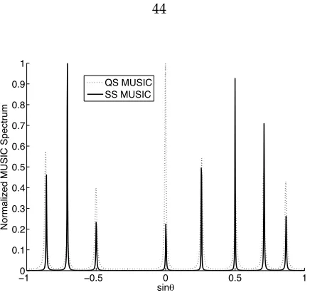
Hereθdenotes the elevation angle andφdenotes the azimuthal angle as represented in Fig. 1.1. Consider an array ofMsensors where the position vector of themth sensor is given bydm∈R3.
PLANE WAVE
θ
ϕ
dm
€ v (θ,φ)
Z
Y
X
Figure 1.1: Figure showing plane wave propagating along the directionv(θ, φ)and received by an array of sensors. Hereθdenotes the elevation andφdenotes the azimuthal angle.
The signal received at theM sensors can be represented as a vector
y(t) =
f(t−τ1)
f(t−τ2) .. .
f(t−τM)
, f(t−τi),f(t;dm), τm= 1
cv
T
dm (1.2)
wherecis the velocity of propagation in the medium andvis as in (1.1). For a narrowband signal model, we can write
whereωcrepresents the carrier frequency (in radians/s) ands(t;d)is the complex envelope with a bandwidth ofBs. In array processing, anarrowbandsignal model is defined as one where
max m τm
1
Bs
This is true if the bandwidthBsof the envelope is considerably small. Under this assumption,
s(t−τm)≈s(t), ∀mand (1.2) reduces to
y(t) =a(θ, φ)s(t)ejωct (1.3)
wherea(θ, φ)∈ CM×1is defined as thesteering vectorof the antenna array and its elements are
given by ωc
c v Td
m,1 ≤ m≤M. Equation (1.3) is widely known as the narrowband signal model for far field wave propagation for a single source. For multiple plane waves propagating through a linear medium, the superposition principle applies. ConsiderDplane wavesfk(t;d)with propa-gation vectors given byv(θk, φk), k= 1,· · ·, D. With additive noisen(t)∈CM×1at theM sensors,
the signal model given by (1.2) becomes
y(t) = D
X
k=1
fk(t−τ (k) 1 )
fk(t−τ (k) 2 ) .. .
fk(t−τM(k))
+n(t) (1.4)
and the narrowband model (1.3) becomes
y(t) =A(Θ,Φ)s(t) +n(t) (1.5) whereA(Θ,Φ) ∈ CM×D is known as theArray Manifoldmatrix whose columns are comprised
ofDsteering vectorsa(θk, φk), k = 1,· · ·, D, and the vectors(t)∈ CD×1contains theD complex
envelopes. For the special case of1D arrays, the position vectors of the elements are given by
vector corresponding to the direction(θ, φ)depends only on the elevation angleθand is given by
a(θ) =
jπd1sinθ
ejπd2sinθ
.. .
ejπdMsinθ
1.1.1.2 Autocorrelation and Spectral Estimation
The spatio-temporal signal model received by an array of sensors often has a statistical representa-tion. For the narrowband signal model, this implies that the waveforms{sk(t)}Dk=1are represented as jointly Wide Sense Stationary (WSS) random processes with a correlation matrix
Rss(τ),E[s(t)s(t−τ)] (1.6) For narrowband signal model, the signals are primarily temporal stochastic processes. However, for wideband signals, the model corresponds to a random field [96] and the autocorrelation matrix of WSS s(t;d) has a spatio-temporal structure Rss(τ,δ) = E[s(t;d)s(t−τ;d−δ)]. Under the narrowband WSS assumption, the autocorrelation matrix is given by
Ryy(τ) =A(Θ,Φ)Rss(τ)AH(Θ,Φ) +σ2nI
(also called pseudo-spectrum) from the autocorrelation function.
1.1.2
Parametric Estimation
The random multichannel signal modely(t)carries bothspatial and temporal informationin the form of unknown quantities of interest such as the number of sourcesD, the Directions of Arrival (DOA) {(Θk,Φk)}Dk=1, the signal waveformssk(t), and the noise powerσ2n. A central goal in array process-ing is to develop powerful algorithms to estimate or extract information from the spatio-temporal observation.
The parametric approach to estimation assumes a probabilistic model for the underlying signal and applies Maximum Likelihood (ML) estimation to extract the unknown parameters of the dis-tribution. Two different assumptions about the source signalss(t)lead to different ML approaches. They are known as deterministic ML (DML) and stochastic ML (SML) algorithms. For the deter-ministic model, the source signals are modeled as unknown deterdeter-ministic quantities and the ran-domness ofy(t)in (1.3) is entirely due to the noise with unknown varianceσ2n. Modeling the noise as spatially white circularly symmetric Gaussian random vector, one can derive the Deterministic ML (DML) estimate [195]( ˆΘ,Φˆ,σˆ2
n,{s(t)}Lt=1)as one that maximizes the log-likelihood function computed overLtime samples
−Llogσ2n+ 1
σ2 nL
L
X
t=1
ky(t)−A(Θ,Φ)s(t)k2
The stochastic approach however consists of modeling the sources as jointly WSS Gaussian random processes with covariance matrixRss. The negative log likelihood function is shown proportional to [17]
1
L
L
X
t=1
kΠ⊥A(Θ,Φ)y(t)k2
ac-curacy, robustness and optimality (in terms of achieving CRB), they are computationally expensive and require multidimensional search over the parameter space. In contrast, the spectral methods as described below provide a computationally attractive and simpler alternative to the ML methods.
1.1.3
Spectral Estimation
As mentioned earlier, the spectral approaches largely operate on the spatial correlation matrixRyy and compute spectrum-like functions for estimation of the parameters of interest. They can be broadly classified as (a) beamforming, and (b) subspace-based methods. The former is linear while the latter is non linear and has distinct advantages over beamforming.
Beamforming [187] is a spatial filtering technique where the observed signals at the output of
M sensors are linearly weighted by a weight vector w ∈ CM×1 and then summed to produce a
scalar output. In its simplest form, the weight vectorwis chosen to steer the array to a particular direction(θ0, φ0).This is obtained by choosingw=a(θ0, φ0)and computing the output as
z(t) =wHy(t).
By changingwto steer at different directions, one obtains an estimate of the spatial spectrum as
P(θ, φ) =aH(θ, φ) L
X
t=1
x(t)xH(t)a(θ, φ)
A different type of beamforming based on an optimal weighting was proposed by Capon [30, 209] and it is called the minimum variance distortionless beamformer (MVDR) which solves forwas
min
w P(w)
such thatwHa(θ0, φ0) = 1 whereP(w) =wHPL
t=1x(t)x
including the adaptive versions, the interested reader is referred to [187].
In contrast to beamforming, subspace based methods for spectral estimation rely upon the eigen structure of the correlation matrix to estimate the spatial paremeters (DOA) of interest. Pisarenko’s harmonic retrieval [152] was one of the earliest algorithms belonging to this family. However, the MUSIC algorithm [160] is probably the most popular subspace based technique for direction finding which gave rise to a family of other algorithms exploiting the low rank structure of the covariance matrix. The covariance matrixRyy =ARssAH+σ2nI(we drop the dependency ofA onΘandΦ) can be decomposed (via eigenvalue decomposition) intoUsΛUHs +σ
2
nUnUHn.The columns ofUn ∈CM×(M−D)are orthogonal to the range space ofA, denotedR(A). The MUSIC
spatial spectrum is defined as
PM(θ, φ) =
1
aH(θ, φ)Π
na(θ, φ)
whereΠn denotes the projection operator on R(Un).It can be shown that for certain array ge-ometries, the MUSIC spectrum exhibits peaks exactly at the true DOA locations with no false or missing peaks. Note that PM(θ, φ)is not a true spectrum but represents a measure of distance between two subspaces. Also notice that estimating the DOAs now merely involves a2Dsearch over(θ, φ)space. There are several other families of subspace based methods such as ESPRIT, Min-Norm algorithm, Root-MUSIC, IQML etc. One important observation on subspace based methods is that the number of sourcesDneed to satisfyD < M. Beamforming algorithms also have this assumption implicitly. Hence,most estimation algorithms in array processing consider an overdetermined
signal model (1.3) whereM > D. This indicates that the number of sourcesDthat can be resolved is
upper bounded by the number of sensorsM.
1.1.4
Sampling and Underdetermined Estimation
While a large body of literature in array processing only considers the overdetermined signal model, a few lines of work consider the underdetermined model where the number of unknown sources can be actually less than the number of physical sensors. In all these cases,the geometry of
the array or the spatial samples plays a vital role in efficient representation of the underdetermined system.
co-array, can be either a sum co-array for an active sensing system or a difference co-array for a passive sensing system. The number of elements in the co-array plays the primary role in determining how many sources can be resolved. For an array withM physical sensors, both the sum and difference co-array can have uptoO(M2)elements, depending on the geometry of the underlying physical array.
One popular application which explicitly uses a virtual array is that of synthetic aperture radar (SAR) where the effect of an artificial larger aperture is created by virtue of the motion of the radar [165]. The use of sum and difference co-arrays respectively in coherent and incoherent imaging was extensively discussed in [89]. The difference co-array also arises in direction finding problems in array processing when one considers the correlation between the signals received at the output of the antennas. Underdetermined models for direction finding using only the second order statistics (correlation) was proposed in [149, 150] and thoroughly investigated in [1, 2]. They propose the use of special one dimensional array geometry known as the minimum redundancy array (MRA) [126] (we shall review this structure in Chapter 2). Given a fixed number (say,M) of sensors, MRA is theoretically the optimum linear geometry which produces the maximum possible number of elements in the difference co-arraywithout any missing elements in between. However, there is no closed form expression for the structure of the MRA or the number of elements in its difference co-array and hence this geometry is not analytically tractable. Also, there is no obvious way to extend this geometry to higher dimensions, or to the so-called higher order difference co-arrays (which arise in estimation problems utilizing higher order statistics of the signal). In the latter case, a number of different virtual arrays can arise depending on the order of statistics used. They constitute the general class ofhigher order difference co-arrays[42, 43]. In the context of active sensing, MIMO radar [38, 39, 16] explicitly utilizes the concept of a sum co-array to create the effect of a virtual array by transmitting orthogonal waveforms and subsequently processing them with a bank of matched filters at the receiver.
1.1.5
New Questions in Array processing
The preceding discussion on existing approaches to underdetermined estimation in array process-ing brprocess-ings us to the followprocess-ing questions.
which has no closed form) that has a simple structure and is capable of producing O(M2) elements in its difference co-array. Also, it is desirable that the structure can be generalized to higher dimensions and be easily extended to the case of higher order statistics. In this thesis, we will propose such a geometry, namely the nested arrays, which will be shown to satisfy all these conditions.
2. Is there an algorithm that can exploit the co-array? Previous attempts at this problem have used variations of an augmented covariance matrix [1, 2, 149], which, for finite number of measurements, is unfortunately not positive semidefinite and hence does not represent a valid covariance matrix. In this thesis, we will propose a new subspace based algorithm which will produce a positive semidefinite matrix representing the covariance matrix corre-sponding to the co-array even for finite number of snapshots. This algorithm will be shown to be generic enough to be applied to two dimensional arrays, as well as to the case of higher order statistics.
3. Can the ideas in one dimension be extended to multiple dimensions? Array processing in two dimensions (2D) can be considerably different from its one dimensional (1D) counter-part. Also, there can be numerous geometries for spatial sampling in2D, which do not arise in1D. In this thesis, we will show that the proposed nested array can be easily extended to 2Dif we consider sampling on2Dlattices. We will also consider another sampling strategy, namely, coprime sampling, which when extended to2D, necessitates the use of coprime and commuting integer matrix pairs. This gives rise to theoretical questions on the existence and construction of such matrix pairs which will be extensively discussed in Chapter 6.
1.2
Sparse Estimation and Compressive Sensing
The problem of underdetermined estimation has received great attention in recent times particu-larly due to its connection with the theory of sparse sampling and recovery, also popuparticu-larly known as “Compressive Sensing”. Fundamentally, it seeks to solve forx∈CN×1from
y=Ax (1.7)
whereA∈CM×N is a fat matrix withN M. As such, the problem is ill defined and the number
of solutions is infinite. However, with more assumptions on the particularxthat is desired, the problem actually can permit a unique answer. A very common assumption is that ofsparsity.
1.2.1
The Ubiquitous Sparse Model
of multi band signals [125], image and video processing [117, 67], radar [87, 40], multivariate re-gression [130], sparse Bayesian estimation [95], monitoring and inferring from networked data [84], and channel estimation [48, 7].
1.2.2
A Brief Review of Sparse Estimation
Sparse estimation is concerned with finding the sparsestx satisfying (1.7). The problem can be readily solved if we knew which elements inx are non zero. However, lack of this knowledge makes the problem very difficult to solve in a computationally efficient manner. The problem of recovering the sparsest solution to (1.7) is also known as the l0 minimization problem and is often cast as minx:y=Axkxk0 where kxk0 denotes the number of non zero elements in x. This
problem in its most general form is NP hard. An alternative approach is to solve the l1 norm minimization problem: minx:y=Axkxk1 and hope the solution is the same as that obtained from
thel0problem. Thel1normkxk1denotes the sum of absolute values ofxand it is the smallestp such that thep−normkxkpis convex. Thel1minimization problem is a linear program which can be solved efficiently by algorithms with polynomial time complexity. In fact,l1minimization has been used for several decades in order to seek sparse solution to the underdetermined problems. However, for a long time, there was a lack of rigorous analytic results for equivalence of the l1 andl0problems. These results were finally established in the 2000s which led to the emergence of “Compressed Sensing” [24, 56] as an active field of research. It has been shown that under certain conditions on the matrixA, the solution obtained froml1minimization problem is identical to that from thel0norm minimization problem. These conditions are characterized by different properties of the matrixAsuch as mutual coherence [58], Restricted Isometry Property (RIP) [25], Exact Reconstruction Condition (ERC) [177] and the Null Space Property [47]. In the following, we present a brief history of algorithmic developments for sparse estimation over the last few decades.
1.2.2.1 A Brief History of Sparse Recovery Algorithms
neuromag-netic imaging. As an alternative to the convexl1minimization, subspace based techniques such as MUSIC [160] were also introduced for recovery of multi band signals with sparse spectrum [76]. Meanwhile, Matching Pursuit (MP) [122, 52] was introduced as a greedy algorithm for denoising signals in redundant dictionaries. Tibshirani proposed al1regularized least squares minimization LASSO [175] for sparse regression in a noisy setting. In what was to follow, extensions of MP and LASSO would become popular means for sparse recovery with analytically provable guarantees.
It was not until the 2000s that a series of breakthrough results demonstrated that the NP hardl0 minimization problem can be exactly solved by the convexl1minimization problem, under certain conditions on the matrixA. As a result, the field of Compressive Sampling [56, 24] emerged, partly building upon the past work (mostly empirical) on sparse recovery, and largely due to the analytic results on the equivalence ofl0 andl1 minimization. These results are undoubtedly among the most important contributions in recent times. In order to establish the power ofl1minimization in recovering the sparse solution, theoretical guarantees based on mutual coherence ofAwere devel-oped in [59, 60, 58] proving the stability of the BP algorithm in presence of noise. Independently, a series of theoretical results onl1minimization [28, 27, 26] provided sufficient conditions for exact reconstruction of sparse vectors using random measurement matrices, in terms of the newly coined term “Restricted Isometry Property” (RIP) of the matrixA[28, 25]. In particular, it was shown that exact reconstruction ofs-sparse vectors is possible using random matrices as projection operators provided the size of projections isO(slogN). Such analysis was also extended for the noisy sce-nario [27, 26]. The work of Donoho et al established necessary and sufficient conditions for sparse recovery and provided stronger guarantees than RIP by using the notion ofk-neighborlypolytopes [57, 61, 62]. For noisy observations, the performance of LASSO was well studied in [190, 205]. A set of necessary and sufficient conditions were established for the solution of LASSO to yield the true support, either exactly or with high probability. A number of papers have also focused on deriving information theoretic bounds on the possibility of recovering sparse vectors, irrespective of any particular algorithm used. These formulations consider a statistical model and derive prob-abilistic guarantees on the sparse recovery by deriving fundamental relations between number of measurements, size of dictionary, sparsity and the noise level. The results of [189, 5, 172] develop such guarantees.
comparable to the convex counterparts. Most notable among these is the Matching Pursuit (MP) al-gorithm [122]. It was modified to Othogonal Matching pursuit (OMP) [147, 52] in the 1990s to yield superior performance. OMP was revisited by Tropp [177, 180] in the context of sparse recovery and thoroughly analyzed. A sufficient condition called the Exact Reconstruction Condition (ERC) was proposed under which OMP can exactly solve thel0problem. It was also shown that for random Gaussian ensembles, the number of measurements required by OMP to recover sparse vectors with high probability, is the same as BP.
1.2.2.2 Extensions
While most algorithms cast the sparse recovery problem in a deterministic setting, a few of them considers a Bayesian approach for the sparse estimation problem. The work in [176, 95, 199, 207] belongs to this class of algorithms. They use a sparse Bayesian learning approach to formulate a MAP estimate for the sparse unknown vector. The sparsity is explicitly characterized in terms of a weight function (which can be zero) on the distribution ofxand it is considered as a hyper-parameter in the estimation problem which can be “learnt” via various approaches. The learning algorithms can be shown to enforce sparsity and recover the true solution. This body of work con-stitutes an alternative to the majority of existing work on convex relaxation based sparse recovery techniques.
sparse recovery by using multiple hypothesis testing framework and also derived a converse re-sult by using information theoretic argument.
1.2.3
New Questions in Sparse Estimation
In this thesis, we will address some new questions in sparse estimation from a statistical point of view. Bayesian approaches to compressive sensing [95, 176] provide one way of incorporating a statistical model and form a fundamental connection between statistical estimation and sparse reconstruction theory. This perspective gives rise to many new questions that can be asked beyond the purview of existing sparse sampling and recovery techniques. In this thesis, we will specifically ask the following questions and explore new possibilities along their lines:
1. What kind of priors can we exploit besides sparsity? The solution to underdetermined systems becomes unique under the prior knowledge about sparsity of the solution. In the literature, several other forms of prior have been considered such as non uniform support [99], partial knowledge of support [188], model based approaches [9] or use of rank of the data [53]. However, the statistical framework offers the possibility of using a much wider variety of priors. In this thesis, we will consider such a prior in terms ofcorrelation between the
variablesand develop new theoretical guarantees.
2. How can we reduce the requirement on the number of samples?The answer to this question will constitute a major contribution of this thesis. Almost every approach to sparse recovery, deterministic or Bayesian, seems to indicate that the number of samples M cannot be less than the sparsity level to be recovered. But, we will show that by designing suitable sampling schemes, it is possible to recovery sparsity levels as large asO(M2)by exploiting the statistical priors.
1.3
Outline and Scope of the Thesis
In this dissertation, we visit the relatively less explored frontiers of underdetermined estimation theory in the context of statistical signal processing as well as sparse reconstruction theory. There are two main problems considered in this thesis. The first problem of focus is estimation in antenna array processing (Chapters 2, 3, 4, 5 and 6). We consider a strictly underdetermined signal model where the number of sensors or antennas can be considerably fewer than the number of unknown spatial parameters. Different variations of this problem are studied. They include correlation based direction finding and extension to distributions with higher order statistics, beamforming and di-rection finding for wideband signals, and didi-rection finding for two dimensional arrays. We propose novel spatial sampling structures in one and multiple dimensions and develop new algorithms to solve the underdetermined estimation problem in an efficient and systematic fashion. The second part of the thesis considers the problem of sparse recovery in compressive sensing (Chapters 7 and 8). By introducing a statistical framework to this problem, we will develop new results for the problem of sparse sampling and reconstruction which will be shown to have better performance guarantees than existing ones. Below is a brief description of the scope of each chapter.
1.3.1
Nested Arrays in One Dimension (Chapter 2)
structure is derived for maximizing the degrees of freedom offered by such an array. It is shown to be order optimal over any array geometry in terms of the maximum number of resolvable sources using only the correlation of the data. We also develop a new subspace based algorithm which is capable of estimating the directions of arrival from the covariance matrix of the nested array. Fur-ther applications of the nested array for beamforming in the power domain are also demonstrated. The nested array thereby provides a new sampling approach to array processing with more sources than sensors.
1.3.2
Nested Arrays in Two Dimensions (Chapter 3)
In Chapter 3, we extend the1Dnested array to two dimensions for two dimensional (2D) direction finding (elevation and azimuth) problems [142, 143].2Darray processing differs considerably from that in one dimension due to some unique problems that arise only in two dimensions. Among many possible sampling geometries in2D, we focus on lattices and propose a family of two di-mensional Nested Arrays on Lattices. The concept of1Dnested array is extended to2D lattices via integer matrices. Various orientations of the proposed structure are considered and optimized. It is further shown that the construction of nested arrays for separable and non separable lattices can be directly related via Smith Form of integer matrices. We also develop a new subspace al-gorithm for2Ddirection estimation using the nested structure. One of the unique issues in two dimensions is the absence of exact conditions on parameter identifiability. We address this prob-lem and develop new insights into two dimensional parameter identification and prove guarantees for different scenarios.
1.3.3
Higher Order Statistics and Extension of Nested Arrays (Chapter 4)
proportional to the order of the statistics used. However, the size also depends on the underlying physical array and the ULA is again shown to be a sub-optimal choice. We propose an extension of the nested array which works for every order of statistics and the size of its virtual array is shown to be order optimal. This demonstrates the flexibility of the proposed nested array in being adapted to every order of statistic. The subspace algorithm proposed in Chapter 2 is also shown to be extensible to this case and it can provably resolve larger number of sources than the previously known algorithms. We also revisit Cramer Rao Bound analysis for underdetermined estimation and examine its applicability to the current model under both deterministic and stochastic setting. The performance of the extended nested array coupled with the new subspace algorithm is shown to be significantly better than previously known approaches, particularly when large number of temporal samples are available.
1.3.4
Wideband Beamforming and Estimation (Chapter 5)
The problems of direction finding and beamforming for wideband signals are significantly dif-ferent from their narrowband versions. This is due to the fact that the response of the array is different at every frequency and incorporation of the information from all different frequencies in the most effective way remains a challenging task. In Chapter 5, we propose two new approaches for wideband array processing. One of them focuses on direction finding from wideband signals [131, 132]. The other one explores new directions in frequency invariant beamforming where the goal is to make the beampattern of the array appear identical across the frequencies. Our approach to wideband direction finding is based on coherently combining the signals in the subbands before performing the estimation. Usually such combination requires some coarse estimtates of the direc-tions. However, we propose a new approach to coherent combination DOA estimation which does not require such estimates. This approach, called autofocusing, is shown to provide better perfor-mance when the coarse estimates are not available. In the second part, we develop new approaches
tofrequency invariantbeamforming using2Dlattices for wideband signals. Wideband beamforming
1.3.5
Commuting Coprime Matrix Pairs (Chapter 6)
Coprime sampling [184, 185] has been recently proposed as a sub Nyquist sampling scheme which enables the autocorrelation sequence to be sampled at the Nyquist rate. Hence, one can employ significantly slower A/D converters (and save power) or deploy fewer sensors and yet retain all the information about the spectrum of the signal. Coprime sampling when extended to two dimen-sions, requires the use of integer matrix pairs which are commuting and coprime. It is challenging to fully characterize the entire family of such matrices. In this chapter, we investigate several fam-ilies of commuting matrix pairs and establish necessary and sufficient conditions for their copri-mality [137]. In particular, we look into circulant, skew circulant, adjugate and triangular pairs of matrices and derive simplified conditions on their entries. The results obtained in this chapter can lead to constructive techniques for commutive coprime matrices.
1.3.6
Correlation Aware Sparse Recovery (Chapters 7 and 8)
to the number of measurement vectors available [145]. This chapter provides a first step towards explicit use of correlation priors in sparse recovery and leads to many future directions for prior aware sparse recovery techniques.
1.4
Notations
Matrices are denoted by uppercase letters in boldface (e.g.,A). Vectors are denoted by lowercase letters in boldface (e.g.,a). SuperscriptH denotes transpose conjugate, whereas superscript∗ de-notes conjugation without transpose. The notation[A]i,jdenotes the(i, j)th elements of matrixA. For a setS,| S |denotes its cardinality. Similarly, given two setsS1andS2,S1\S2 denotes the difference of the sets,S1∩S2denotes their intersection andS∪S2denotes their union. Given a set of integersS⊂ {1,2,· · ·, N}and a vectorv∈CN×1, the vector[v]S ∈
C|S|×1consists of elements
ofvindexed byS. Similarly given a matrixA∈ CM×N, the matrixAS ∈CM×|S|consists of the
columns ofAindexed byS.
The symboldenotes the Khatri-Rao product [186] between two matrices of appropriate size and the symbol⊗is used to denote the left Kronecker product (p.1353of [186]). For two matrices
AandBof same dimensions,A◦Bdenotes the Hadamard product [91]. For example, consider
2×2 matricesA ∈ CM×N =
a1 a2
a3 a4
andB ∈ C
M×N =
b1 b2
b3 b4
. Then, the Kronecker,
Khatri Rao, and Hadamard products are respectively given by
A⊗B=
Ab1 Ab2
Ab3 Ab4
, AB=
a1b1 a2b2
a1b3 a2b4
a3b1 a4b2
a3b3 a4b4
, A◦B=
a1b1 a2b2
a3b3 a4b4
Chapter 2
Nested Arrays in One Dimension
2.1
Introduction
In this chapter, we will consider a classical parameter estimation problem, namely simultaneous direction finding using antenna arrays. Contrary to the traditional scenario, we will consider the case where the model is highly underdetermined. This happens when the number of spatial sam-ples of the impinging electromagnetic waveform (equivalently the number of antennas) is less than the number of unknown directions to be resolved. We will develop a systematic theory of such an estimation problem and propose a new antenna geometry which is fundamentally capable of resolving more sources than the number of antennas. This underdetermined model will be revis-ited in Chapter 7 in the context of finding sparse solutions for linear underdetermined system of equations. This problem arises in a wide variety of applications such as sub Nyquist sampling and reconstruction, multivariate regression, imaging, source localization etc. The proposed spatial nested sampling will be shown to play an important role in such problems as well.
hence can resolve significantly more sources than the actual number of physical sensors. We call this class of arrays as “nested arrays” because they are obtained by combining two or more ULAs with increasing inter-sensor spacing. We shall demonstrate that using only second order statistics of the impinging sources, it is possible to obtainO(N2)DOF from onlyN physical sensors.
The main idea behind the ability to resolve more sources than physical sensors is based upon the concept of adifference co-array. This helps in performing array processing with increased de-grees of freedom in a completely passive scenario. The difference co-array becomes visible as one computes the correlation between the signals received at the different antennas. Hence the new direction finding and beamforming algorithms proposed in this chapter work entirely in the cor-relation domain. The co-array concept has previously been treated for specific array geometries in [89],[103]. In Section 2.5, we propose our nested array structure which can greatly increase the degrees of freedom of the corresponding co-array. It will be shown in Section 2.5 that the nested array is extremely easy to construct and it is possible to provide exact closed form expressions for the sensor locations and the degrees of freedom for a given number (N) of sensors, unlike the so called Minimum Redundancy Arrays (MRAs) used in [149, 1, 2]. We shall also propose a novel spatial smoothing based technique in Section 2.6 which utilizes only second order statistics to ex-ploit the degrees of freedom offered by the array and works well even for stationary sources. Our technique constructs a suitable covariance matrix (which we shall refer to as the spatially smoothed matrix) corresponding to a longer array on which subspace based methods can be applied directly to perform detection and estimation of more sources than sensors.
As another potential application of the signal model based on the nested array, a new approach to beamforming is proposed in Section 2.7, which directly makes use of the degrees of freedom offered by the co-array. This approach spatially filters thepowerof the sources (instead of their am-plitude) and hence it is inherently non-linear in nature. Another major advantage of the proposed approach to beamforming is that, assuming perfect knowledge of the signal covariance matrix, it can eliminate noise, which is never possible using conventional linear approach to beamforming. It should be pointed out that the proposed spatial smoothing based method as well as the beam-forming are applicable to any array whose difference co-array is a filled ULA and hence they can be applied even to MRAs.
arrays [126] and an augmented covariance matrix, degrees of freedom can be improved. How-ever, the constructed augmented covariance matrix is not positive semidefinite for finite number of snapshots (and hence violates the condition for being a covariance matrix.) Unlike the augmented matrix in [149], the spatially smoothed matrix proposed in this thesis isguaranteed to be positive
semidefinite for any finite number of snapshots. In [1],[2], a transformation of the augmented matrix
into a suitable positive definite Toeplitz matrix was suggested and an elaborate algorithm was pro-vided to construct this matrix. However, there are two issues with this approach. To gain more degrees of freedom required for detection of more thenN −1 sources withN sensors, they rely on the class of Minimum Redundancy Arrays (MRAs), for which, unfortunately, there is no closed form expression for either the array geometry or the achievable degrees of freedom for a givenN. The optimum design of such arrays is not easy and in most cases, they are restricted to computer simulations or complicated algorithms for sensor placement [96],[110],[148],[159],[39]. Also, the al-gorithm for finding the suitable covariance matrix corresponding to the longer array is a lengthy and complicated iterative algorithm, which converges only to a local optmimum [1, 2]. In [154], the use of fourth order cumulants was suggested to completely remove the Gaussian noise term and perform better DOA estimation. It was later shown that through the use of fourth order cumulants, one can also achieve significant increase in degrees of freedom [63],[42],[43]. But one weakness of this approach is that it is restricted to non Gaussian sources. Recently, using the concept of Khatri-Rao (KR) product and assuming quasi stationary sources, it has been shown that one can identify upto2N −1sources using aN element ULA [118] without computing higher order statistics. It is to be noted that using the augmented array approach of [149] or with the construction of suit-able positive definite Toeplitz matrices as done in [1], it will not be possible to obtain this many degrees of freedom using a ULA. Unfortunately, this method based on quasi stationary sources, is not applicable to stationary signals. In [16], degrees of freedom were increased by generating a virtual sum co-array using a MIMO radar. However, the generation of the sum co-array needs active sensing, i.e., both transmit and receive antennas, and is not applicable to the case of passive sensing.
2.2
Outline
In Sec. 2.3, a new signal model based on the concept of a difference co-array is developed. In Sec. 2.4, we discuss the role of difference co-array of the physical antenna array which plays an important role for resolvingO(N2)sources usingN sensors. In Sec. 2.5, we propose a new array geometry, namely, the nested array and optimize the degrees of freedom offered by it under a fixed budget of available physical sensors. In Sec. 2.6, we propose a new subspace


![Figure 3.1: Fundamental parallelepiped (FPD) of the lattice generated by the generator matrix V[ =v1v2]](https://thumb-us.123doks.com/thumbv2/123dok_us/1120513.1141180/81.612.235.417.258.368/figure-fundamental-parallelepiped-fpd-lattice-generated-generator-matrix.webp)