Volume 2008, Article ID 593216,10pages doi:10.1155/2008/593216
Research Article
Adaptive S-Method for SAR/ISAR Imaging
LJubiˇsa Stankovi´c,1Thayananthan Thayaparan,2Vesna Popovi´c,1Igor Djurovi´c,1and Miloˇs Dakovi´c1
1Electrical Engineering Department, University of Montenegro, 81000 Podgorica, Montenegro
2Radar Applications and Space Technology, Defence Research and Development, Ottawa, Ontario, Canada K1A 0Z4
Correspondence should be addressed to Igor Djurovi´c,[email protected]
Received 8 June 2007; Accepted 8 November 2007
Recommended by Sven Nordholm
We propose the adaptive S-method-based technique for imaging of SAR and ISAR targets. This approach can be applied in the 1D and 2D modes. It is a postprocessing technique, since the first stage is the standard radar imaging with the 2D Fourier transform. In addition, selection of the adaptive parameter in this technique is efficient and can be performed based on simple rules in real time. The proposed technique produces highly concentrated (focused) radar image without interferences commonly associated with time-frequency representations and without defocusing target images that are already focused in the 2D Fourier domain.
Copyright © 2008 LJubiˇsa Stankovi´c et al. This is an open access article distributed under the Creative Commons Attribution License, which permits unrestricted use, distribution, and reproduction in any medium, provided the original work is properly cited.
1. INTRODUCTION
When radar transmits an electromagnetic signal to a tar-get, the signal reflects from it and returns to radar. The re-flected signal, as compared to the transmitted signal, is de-layed, changed in amplitude, and possibly shifted in fre-quency. These parameters of the received signal contain in-formation about the target’s characteristics. For example, de-lay is related to the target’s distance from the radar. The syn-thetic aperture radar (SAR) and the inverse synsyn-thetic aper-ture radar (ISAR) are systems for obtaining high-resolution image of a target based on the changes in viewing angle of the target with respect to the radar. Relative motion between radar and target produces these viewing angle changes. In the case of ISAR, radar is fixed while the target is moving, while in the SAR case radar is carried on an aircraft or spacecraft
platform, moving at uniform speed and constant altitude [1].
Common technique for SAR and ISAR imaging is based on the 2D Fourier transform (FT). This technique is appro-priate for imaging nonmoving SAR targets and for rigid body
imaging of ISAR targets [1–4]. However, for fast
maneuver-ing ISAR targets [1,5] and targets with 3D motion [1,6],
radar image can be spread in the 2D FT domain. Similar
de-focusing effects are observed in the SAR systems for moving
targets [7,8]. In addition, image of moving targets in SAR
systems can be dislocated from the proper position [1,7,8].
An additional problem in both SAR and ISAR systems is the
micro-Doppler effect caused by fast rotation and vibration of
the radar target parts [9,10]. Thus, some more sophisticated
techniques should be employed for focusing radar images. One group of techniques is based on the motion compen-sation. These techniques may be based on direct estimation of the target motion parameters, or these parameters can be extracted indirectly by estimating parameters of received sig-nals. Excellent results can be achieved using these techniques,
but at the expense of the high computational load [11–15].
An alternative group of techniques is based on the
time-frequency (TF) representations [1,10,16]. Some of the most
common TF representations, such as the Wigner distribution (WD), produce highly concentrated signal terms but with drawback in appearance of undesired interference (cross)
terms [17–19]. The S-method (SM), as a TF
representa-tion that can produce significant improvement in imaging of radar targets (as in the WD) without introducing cross-terms (as in the standard 2D FT technique), is proposed recently
[20]. This method has a parameter that represents a
win-dow width in the frequency domain [21]. Results achieved
by the SM, although computational simple, may depend on this parameter. Namely, for a very narrow window the ob-tained radar image could still be spread, while for a very wide window the obtained image can be corrupted by cross-terms. In this paper, we propose a technique for adaptive se-lection of the window width in the SM. This technique is
very effective. It is based on simple rules and brings major
2D forms of the adaptive SM are proposed with implementa-tion issues discussed. An important step in the adaptive SM calculation is threshold determination. The threshold value can be determined in various manners. The Otsu algorithm
[22] based procedure for automatic threshold determination
is used here. The proposed technique is tested on several ex-amples of the SAR and ISAR images. Note that special pur-pose hardware for both 1D and 2D adaptive SM is propur-posed
and analyzed in details recently in [23]. All these facts
con-firm that this is a very promising technique for both SAR and ISAR imaging.
The manuscript is organized as follows. Brief review of
the signal model in considered systems is given inSection 2
along with standard imaging techniques. The proposed
tech-nique is presented in Section 3. Results of simulations are
given inSection 4.
2. SIGNAL MODEL
In both SAR and ISAR systems series of signals is transmit-ted toward radar target. Commonly, these signals are chirps (linear frequency modulated (FM) signals), but some other waveforms are also used in practice. After receiving, these signals are demodulated to the baseband with possible dis-tance compensation and some other preprocessing opera-tions (such as pulse compression). Let the preprocessed
re-ceived signal be denoted asq(m,t), wheretis the time
in-dex (so-called fast-time coordinate) whilem∈[0,M)
corre-sponds to the signal number transmitted toward a target (so-called slow-time coordinate). Commonly, for simpler pro-cessing, signal is sampled in the fast-time with the properly
selected sampling intervalq(m,n)=q(m,nΔt).
The received signal for point scatterer model [1,6] can
be presented as a sum of the FM signals:
q(m,n)=
i
σiexp
jφi(m,n), (1)
whereσi is reflection coefficient of the corresponding
scat-terer. Form of the phase functionsφi(m,n) depends on the
type of the corresponding radar scatterer. Here, we will give approximative forms of the phase function for some typical cases in both SAR and ISAR systems.
(1) For nonmoving targets in SAR systems and for con-stant velocity targets in ISAR systems, the phase func-tion can be approximated by:
φi(m,n)=a(1)i m+b
(1)
i n. (2)
So, the received signal is a 2D complex sinusoid. (2) Phase function of moving targets in the SAR systems
is analyzed in [1]. Similar results are observed in some
ISAR systems with uniform acceleration of targets:
φi(m,n)=a(2)i m2/2 +a
(1)
i m+b
(1)
i n. (3)
Corresponding signal is the linear FM one alongmand
complex sinusoid alongn.
(3) Recent surveys in [24, 25] have shown that returns
from nonuniform moving targets in the SAR systems
can be accurately represented only with higher-order polynomial phase FM signals:
φi(m,n)=
P
p=1 a(ip)
mp
p! +b (1)
i n, (4)
whereP >2.
(4) ISAR targets with fast and 3D maneuvers can produce phase function of the form
φi(m,n)=a(1)i m+b
(1)
i n+ P
p=1
K
k=1 di(p,k)
mp
p!
nk
k!, (5)
where parameters in slow and fast-time cannot be treated as independent like in the previous cases. (5) For fast rotating or vibrating parts of the SAR/ISAR
target, the phase function can be modeled as a sinu-soidally modulated FM signal:
φi(m,n)=a(1)i m+b
(1)
i n+cisin
αim+βin+ϕi
. (6)
In all considered cases, the phase functions can be written as
φi(m,n)=a
(1)
i m+b(1)i n+ψi(m,n), whereψi(m,n)
repre-sents higher-order terms in the signal phase, while
parame-ters (a(1)i ,bi(1)) correspond to the position of scatterers. Other
introduced parametersa(ip),d
(p,k)
i ,ci,αi,βi, andϕidepend on
the position of the targets, relative motion, radar systems pa-rameters, parameters of the target motion, and some other
effects.
The radar image can be obtained by using the 2D FT1as:
Qm,n=
m
n
q(m,n)w(m,n)
×exp−j2πmm/M−j2πnn/N, (7)
whereNis the number of samples in the fast-time direction,
whilew(m,n) is a window function used to reduce spectral
leakage effects in the FT domain. For a single scatterer return
that corresponds to the nonmoving targets in the SAR sys-tems and rigid body parts in the ISAR syssys-tems (case 1) the 2D FT is
Qi
m,n=σiW
m−Ma(1)i /2π,n−Nb
(1)
i /2π
, (8)
whereW(·) is 2D FT of the window function. Since a
win-dow is commonly designed to be highly concentrated in the FT domain, we can assume that, for stationary targets, radar image is highly concentrated around position that is
propor-tional to (a(1)i ,b(1)i ), and these parameters are proportional
to the position of the scatterer point.
For other forms of the phase function the 2D FT can be represented in the following form:
Qi
m,n=σiW
m−Ma(1)i /2π,n−Nb(1)i /2π
∗m∗nFTexpjψi(m,n),
(9)
1Recently, backprojection techniques are used for the SAR imaging. Since
where ∗m∗n represents 2D convolution, while the term
FT{exp(jψi(m,n))}causes spreading and possible
dislocat-ing component from the proper position. The motion com-pensation techniques compensate this term based on the es-timation of motion parameters of the targets. Alternatively, it
can be performed by estimating higher-order coefficients in
the signal phase [11–15]. However, these techniques are very
computationally demanding. The TF representations are an-other approach that will be considered in the next section.
3. RADAR IMAGING BY USING TF REPRESENTATIONS
3.1. Background
It has already been shown that the imaging based on the 2D FT causes spreading of radar images. In order to avoid complex valued nature of the 2D FT, its squared magnitude |Q(m,n)|2
is commonly used for imaging that is equiva-lent to the periodogram in spectral analysis (or to the spec-trogram in the TF analysis). In the TF analysis, the WD is a tool that can be used to improve concentration of the radar image, that is, to reduce spreading. However, the WD has a serious drawback in the form of appearance of spurious com-ponents called cross-terms. The cross-terms may be so em-phatic that they mask the useful components. Then, design of the TF representations that have more concentrated com-ponents than in the standard image but without undesired
effects is the goal of this paper.
3.2. SM
The SM is technique widely used in the TF analysis for cross-terms free TF representation (or representation with reduced cross-terms) giving highly concentrated TF
compo-nents [26]. The SM can be defined for radar images as [20]
SM1
m,n=
k
Π(k)Qm+k,nQ∗m−k,n,
(10)
whereΠ(k) is window in the frequency domain. For fixedn
this form is the 1D SM for fixed-range cell. In similar manner, radar image based on the 1D SM for fixed cross-range cell is
[20]
SM2
m,n=
l
Π(l)Qm,n+lQ∗m,n−1.
(11)
Also, the 2D SM is [20]
SM3
m,n=
k
l
Π(k,l)Qm+k,n+l
×Q∗m−k,n−l.
(12)
Commonly, the frequency window function is rectangular,
and for 1D SM given with (10) exhibits
Π(k)= 1, |k| ≤K,
0, elsewhere. (13)
Then, the corresponding SM form can be calculated as
SM1
m,n
=Qm,n2+ 2Re
K
k=1
Qm+k,nQ∗m−k,n
.
(14)
ForK = 0 we obtain the standard radar image (defocused
but without spurious terms), while for large K the radar
image approaches the WD-based image (focused but with
interfering cross-terms). Fortunately, for relatively smallK
the radar image could be significantly improved without in-troducing the interference. A drawback of this technique is demonstrated in the next subsection on a simple example.
3.3. Illustrative example
Consider three point targets. The first and third targets are moving with constant velocity in SAR (equivalent to the uni-form acceleration in ISAR), while the second is nonmoving target in SAR (equivalent to the constant velocity in ISAR). The returned radar signal from these three targets can be
modelled as (Section 2)
x(n)=A(n)e−j(0.4/256)πn2
e−j(π/2)n+A(n)ej(π/8)n
+A(n)ej(0.2/256)πn2
ej(π/3)n, (15)
where the amplitudeA(n) is slow-varying, defined asA(n)=
1/2 + (1/2) cos(2π/256)n. The signal is observed for−128≤
n ≤ 127. For the considered time instantn = 0, it will be
ω1(0)= −π/2,ω2(0)=π/8, andω3(0)=π/3.
The spectrogram of the analyzed signal is shown in Figure 1(a). The first and third targets are spread and not vis-ible compared to the second target. Note that the radar signal returned from the second target is constant-frequency com-ponent, while the radar signals returned from the first and third targets are linear FM.
The spectrogram corresponds to the SM withK = 0.
By increasing the value ofK concentration of the first and
third targets is improved,Figure 1(b)K = 4, but these
tar-gets are still spread compared to the second one. For higher
value ofK,K =16, concentration of the components
con-tinue to increase, but the cross-term appears between close
targets, the second and third inFigure 1(c). The desired
con-centration of the first and third components is achieved by
using the WD, SM with K equal to the signal length, but
this value generates very strong cross-terms between
com-ponents, see Figure 1(d). The cross-term between the
0.5 0
−0.5
Normalized frequency
−20 0 20 40 60 80 100
M
ag
nitude
(a)
0.5 0
−0.5
Normalized frequency
−20 0 20 40 60 80 100
M
ag
nitude
(b)
0.5 0
−0.5
Normalized frequency
−20 0 20 40 60 80 100
M
ag
nitude
(c)
0.5 0
−0.5
Normalized frequency
−20 0 20 40 60 80 100
M
ag
nitude
(d)
0.5 0
−0.5
Normalized frequency 0
20 40 60 80 100
M
ag
nitude
(e)
0.5 0
−0.5
Normalized frequency 0
5 10 15 20 25 30 35
K
(f)
Figure1: Representation of the three-component signal by using: (a) spectrogram (S-method withK=0), (b) S-method withK=4, (c) S-method withK=16, (d) Wigner distribution (S-method withKequal to the signal length), and (e) adaptive S-method. (f) Values ofK used for obtaining the adaptive S-method.
technique for radar imaging in order to achieve high concen-tration without interferences. Fortunately, one possible so-lution, the adaptive SM, is quite simple. The resulting
rep-resentation of the analyzed signal is given in Figure 1(e).
Here, we assumed that value of K depends on the
con-sidered frequency. It can be observed that high values of
K are used where concentration improvement is necessary
(aroundω1(0) andω3(0)), while in the case when the
com-ponent is well concentrated in the spectrogram, very low
values of K (or K = 0) are used. In the next subsection
3.4. Adaptive 1D SM
Here, we give a form of the adaptive SM for fixed-range cell, but in the same manner it can be evaluated for fixed cross-range cell. The adaptive SM is originally developed for
im-proving the TF representation in [21].
The adaptive 1D SM for radar images can be defined as
SM1
m,n
=Qm,n2+2Re
K(m,n)
k=1
Qm+k,nQ∗m−k,n
.
(16)
The main problem here is determination of K(m,n).
K(m,n) can be simply obtained as a maximal value ofkfor
which the term Re{Q(m+k,n)Q∗(m−k,n)}used for the
SM calculation is greater than a specific thresholdR(m,n),
and where all Re{Q(m+k,n)Q∗(m−k,n)}for|k|<|k|
are greater than the threshold. This can be written as
Km,n
=arg max
k k
k=1
ReQm+k,nQ∗m−k,n≥Rm,n,
(17)
where∧k
k=1represents logical operation AND applied to
log-ical expressions from argument for variousk=1,. . .,k.
The threshold value can be determined in various ways.
The global threshold is proposed in [21] as
R=εmax
m,nQ
m,n2, (18)
whereεcan be adopted as a small value, for example,ε ∈
[0.1%, 5%]. Of course, this threshold can be calculated in
the same manner for considered range or cross-range cell. In this way components having small energy are removed and they are indication of the end of the useful radar component. In the case of images corrupted by a noise we can select global threshold as
R=maxεmax
m,nQ(m ,n)2
,κ2σ2m,n, (19)
whereσ2(m,n) is variance of the radar image caused by the
noise. An analysis of noise in the SM can be found in [27]. In
this case we can remove all weak components, as well as the
components influenced by noise. Parameterκis commonly
selected to be aroundκ=3 (three sigma rule).
This thresholding approach can be applied locally for re-gions of the radar image. In addition, well-described tech-niques from the digital image processing can be used in this
application [22]. The procedure for the threshold
determi-nation based on the Otsu algorithm [22, pages 598–600] is
used here. The 2D FT magnitude|Q(m,n)|is taken as
im-age pixels intensity needed for the algorithm.
Step 1. Estimate initial value for threshold. Here, initial value
for threshold is set to the half of the pixels intensity maxi-mum:
ρ=1
2maxm,nQ
m,n. (20)
Step 2. Calculate two sumsS1 andS2, whereS1 is a sum of
intensity values of the pixels whose intensity is larger than
the current thresholdρ:
S1=
m,n Q
m,n| ∀m,n,Qm,n|> ρ,
(21)
whileS2is a sum of intensity values of the pixels whose
in-tensity is smaller than the current thresholdρ:
S2=
m,n Q
m,n ∀m,n,Qm,n< ρ.
(22)
Step 3. Calculate two new thresholds,ρ1andρ2, as average
values of the obtained sums:
ρ1= S1 N1
, ρ2=
S2 N2
, (23)
whereN1andN2 are number of elements summed in (21)
and (22), respectively.
Step 4. Compute a new threshold value
ρ=1 2
ρ1+ρ2. (24)
Step 5. Repeat Steps2through4until the difference inρin
successive iterations is smaller than a predefined parameter, or for a specified number of iteration.
The thresholds used in our simulations are obtained after
five iterations. Its squared value,R=ρ2, is used in both 1D
and 2D adaptive SM calculation.
3.5. Adaptive 2D SM
The adaptive 2D SM can be evaluated as [28]
SM3
m,n =Qm,n2
+2Re
K(m,n)
k=0
L(m,n)
l=1
Qm+k,n+lQ∗m−k,n−l
+2Re
K(m,n)
k=1 0
l=−L(m,n)
Qm+k,n+lQ∗m−k,n−l
.
(25)
Here, we have to determine two adaptive valuesK(m,n)
andL(m,n) for each pixel in the radar image. However,
multiparameter optimization in this case is difficult and it
could lead to nonoptimal solutions. Instead, we will use
I(m,n) = K(m,n) = L(m,n), so just one adaptive
value for width of the used square window has to be
deter-mined. The adaptive square window width I(m,n) = I
for the considered radar image pixel can be determined as
a maximal value of I for which all terms Q(m +k,n+
Table1: The motion parameters for the targets used in the SAR example.
Scatterer no. 1 2 3 4 5 6 7 8
x0[m] −34 0 34 −34 34 −34 0 34
y0[m] 120 120 120 0 0 −120 −120 −120
vx
m
s
−25 0 −30 0 40 0 0 0
vy
m
s
40 30 −30 60 0 20 30 −50
ax
m
s2
0 0 2 0 0 0 0 0
ay
m
s2
1 0 0 0 0 0 0 1
the used square window) are greater than a specific threshold
R(m,n). This can be written as
Im,n=arg max
I I
k,l=1
Qm+k,n+lQ∗m−k,n−l
≥Rm,n.
(26)
The adaptive 2D SM can improve concentration of the radar image using information from both the range and cross-range cells and it can be useful in the case of images with significant spreading in both directions. This spreading can occur in the case of very complicated maneuvers or in the case when radar and target are relatively close to each other, and also in some other setups.
Now, we overview all advantages of the proposed tech-niques. The adaptive SM is a postprocessing technique that modifies standard radar image calculated by using the 2D FT. Additional processing consists of two parts: threshold evalu-ation and adding terms to the standard radar image. Both these steps require just a moderate calculation burden since they consist of simple multiplications, additions, and logi-cal operations. In addition, hardware realization of the SM is
well developed for both 1D and 2D signals [23]. This
hard-ware requires just a moderate modification to be used in
the proposed application. As it will be seen fromSection 4,
achieved results with the SM are quite accurate and we see this approach as one of the main candidates to be used as a
trade-offbetween accuracy and quality of radar images and
computational demands.
4. EXAMPLES
In this section we illustrate the advantages of the proposed technique on the two examples for SAR and ISAR images ob-tained by using simulated setups. Application of the adaptive 1D SM to the MIG target model is also illustrated at the end of the section.
4.1. SAR example
The eight targets setup, where each target can be modeled as point scatterer, is considered in this example. Radar sig-nal reflected from the 8 point scatterers can be obtained by using superposition principle as a sum of individual echoes.
All targets are moving. The position of the radar targets
can be described as xi(t) = xi0+ vxi(0)t+ (1/2)axit2 and
yi(t)=yi0+vyi(0)t+(1/2)ayit2, where the motion parameters
are given inTable 1.
The radar parameters of the Environment Canada’s
air-borne CV 580 SAR system described in [24] are used as a
basis for this example. The radar operates at the frequency
f0=5.3 GHz, which corresponds to the frequency of C-band
of the CV 580 SAR system. The bandwidth of linear FM
sig-nals isB=50 MHz, the pulse repetition time isT=1/300 s,
with M = 256 pulses in one revisit. Number of samples
within one pulse is N = 256. The aircraft with a radar is
moving alongx-axis with velocityV =130 m/s. Radar
alti-tude ish=6 km, while radar ground distance to the target is
9400 m.
The conventional SAR image is obtained by 2D FT
pro-cessing and it is shown in Figure 2(a). Since all targets are
moving, the obtained radar image is blurred, while some of the targets are also dislocated from the true position. By ap-plying the signal independent 1D SM-based postprocessing of the obtained 2D FT, the resulting radar image will be more
focused,Figure 2(b). By increasing the value ofK(in this
ex-ampleK = 8 is used), the improved concentration is
ob-tained. The 1D SM will produce good performance in the case when the targets are not very close. In the case of close targets (no. 1 and no. 2, and no. 6 and no. 7), the undesired cross-terms will appear between them as a result of its mu-tual influence. The SAR image obtained by using the adaptive 1D SM will result in the well-concentrated targets, and
with-out undesired cross-terms, seeFigure 2(c). Here, the SM and
the adaptive SM are calculated along the cross-range. Since target velocities induce spreading in the cross-range, focus-ing along this axis is needed. Spreadfocus-ing along range direc-tion can also appear in convendirec-tionally processed radar
im-age, see Figure 2(a). This spreading appears as a result of
fast moving targets and radar setup. In this case, the adap-tive 2D SM should be used. Namely, information from both range and cross-range cells are used for adaptive 2D SM
cal-culation. Achieved results are shown inFigure 2(d). The
150 100 50 0
−50
−100
−150
Cross-range
−150
−100
−50 0 50 100 150
Range
(a)
150 100 50 0
−50
−100
−150
Cross-range
−150
−100
−50 0 50 100 150
Range
(b)
150 100 50 0
−50
−100
−150
Cross-range
−150
−100
−50 0 50 100 150
Range
(c)
150 100 50 0
−50
−100
−150
Cross-range
−150
−100
−50 0 50 100 150
Range
(d)
Figure2: Simulated SAR image obtained by using (a) 2D FT, (b) 1D SM withK=8, (c) adaptive 1D SM, and (d) adaptive 2D SM.
Table2: The positions of the reflectors used for the ISAR target simulation.
Reflector No. 1 2 3 4 5 6 7
x[m] −3.4642 0 3.4642 1.7320 −1.7320 0 1.5541
y[m] 2.3094 2.3094 2.3094 −1.1547 −1.1547 −4.6189 0.6414
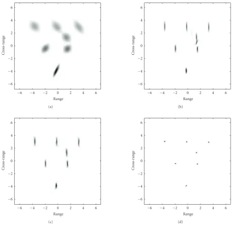
4.2. ISAR example
The radar setup used in [3] is considered as a basis for
this example. The high-resolution radar operates at the
fre-quency f0 =10.1 GHz, the bandwidth of linear FM signals
isB=1410 MHz, the coherent integration time isT =2 s,
withM = 128 pulses in one revisit. The number of
sam-ples within one pulse is N = 128. The target consisted of
seven reflectors is atR=2 km distance from the radar, and
rotates at ωR=4◦/sec. The nonuniform rotation with
fre-quencyΩ=1 Hz,ωR(t)=ωR+Asin(2πΩt), and amplitude
A=1◦/sec is superimposed for each reflector. In addition, all
reflectors have uncompensated range velocity vx = 1 m/s.
The distance between radar and targets after range compen-sation is
di(t)=xicos
θR(t)
+yisin
θR(t)
+vxt, i=1,. . ., 7,
(27)
whereθR(t)=ωRt−A/(2πΩ)cos(2πΩt). The positions for
each reflector at the beginning of the observation interval are
given inTable 2.
The ISAR images obtained by different radar signal
pro-cessing methods are shown inFigure 3. The 2D FT will result
in blurred image, seeFigure 3(a). Improved concentration is
obtained by using the 1D SM, seeFigure 3(b). Here,K =8
is used for the 1D SM calculation. Since some of the reflec-tors are very close, the cross-terms will appear before obtain-ing satisfyobtain-ing concentration. The adaptive 1D SM is used in order to avoid cross-terms, while achieving good
concentra-tion, seeFigure 3(c). It can be seen fromFigure 3(a)that the
6 4 2 0
−2
−4
−6
Range
−6
−4
−2 0 2 4 6
C
ross-r
ange
(a)
6 4 2 0
−2
−4
−6
Range
−6
−4
−2 0 2 4 6
C
ross-r
ange
(b)
6 4 2 0
−2
−4
−6
Range
−6
−4
−2 0 2 4 6
C
ross-r
ange
(c)
6 4 2 0
−2
−4
−6
Range
−6
−4
−2 0 2 4 6
C
ross-r
ange
(d)
Figure3: Simulated ISAR image obtained by using (a) 2D FT, (b) 1D SM withK=8, (c) adaptive 1D SM, and (d) adaptive 2D SM.
using information from both range and cross-range direc-tions, the adaptive 2D SM is applied and the resulting radar
image is shown inFigure 3(d). The resulting radar image is
better concentrated and without undesired cross-terms. The threshold obtained by performing the previously described Otsu algorithm-based procedure is used for the adaptive 2D SM and adaptive 1D SM calculation.
4.3. Application to the MIG target model
The advantage of the adaptive 1D SM is illustrated on the MIG target model. This model is commonly used as a
stan-dard benchmark for comparison of different ISAR
imag-ing methods. The ISAR image of the MIG obtained by
us-ing the 2D FT is shown inFigure 4(a), while the ISAR
im-age obtained after applying the SM withK = 6 is given in
Figure 4(b). The points on the nose of the MIG and the up-per part of the wings are blurred in the ISAR image obtained by using the 2D FT as a result of maneuvers they perform. The points on the tail of the MIG and lower part of the wings are well concentrated and no additional focusing is neces-sary. After the SM is applied to the radar signal, the concen-tration of the target’s points which belong to the nose and upper part of the wings is improved, but cross-terms appear between the close points on the tail of the MIG and lower
part of the wings. InFigure 4(c), the ISAR image of the MIG
(a)
(b)
(c)
Figure4: ISAR image of MIG obtained by using (a) 2D FT, (b) 1D SM withK=6, and (c) adaptive 1D SM.
5. CONCLUSION
An efficient adaptive technique for postprocessing SAR/ISAR
images obtained using 2D FT is proposed. This technique is based on the adaptive 1D and 2D SM. It has been shown that simple strategy for adaptive selection of the frequency win-dow width in the SM produces excellent results with highly focused radar images and with avoiding undesired inter-ference terms. The adaptive selection of frequency window width is an important part of the proposed technique. The threshold determination issue is discussed and the procedure
based on the Otsu algorithm appears to be very efficient.
Nu-merical examples confirm quality of the proposed technique.
REFERENCES
[1] V. C. Chen and H. Ling,Time-Frequency Transforms for Radar Imaging and Signal Analysis, Artech House, Boston, Mass, USA, 2002.
[2] W. G. Carrara, R. S. Goodman, and R. M. Majewski, Spot-light Synthetic Aperture Radar—Signal Processing Algorithms, Artech House, Norwood, Ohio, USA, 1995.
[3] S. Wong, E. Riseborough, and G. Duff, “Experimental investi-gation on the distortion of ISAR images using different radar waveforms,” Technical Memorandum TM 2003-196, Defence Research and Development Canada, Ottawa, Canada, 2003. [4] S. R. DeGraaf, “SAR imaging via modern 2-D spectral
estima-tion methods,”IEEE Transactions on Image Processing, vol. 7, no. 5, pp. 729–761, 1998.
[5] Z. S. Lieu, R. Wu, and J. Li, “Complex ISAR imaging of ma-neuvering targets via the Capon estimator,”IEEE Transactions on Signal Processing, vol. 47, no. 5, pp. 1262–1271, 1999. [6] V. C. Chen and W. J. Miceli, “Simulation of ISAR imaging of
moving targets,”IEE Proceedings: Radar, Sonar and Navigation, vol. 148, no. 3, pp. 160–166, 2001.
[7] R. K. Raney, “Synthetic aperture imaging radar and moving targets,”IEEE Transactions on Aerospace and Electronic Systems, vol. 7, no. 3, pp. 499–505, 1971.
[8] M. Kirscht, “Detection and imaging of arbitrarily moving tar-gets with single-channel SAR,”IEE Proceedings: Radar, Sonar and Navigation, vol. 150, no. 1, pp. 7–11, 2003.
[9] V. C. Chen, F. Li, S.-S. Ho, and H. Wechsler, “Analysis of micro-Doppler signatures,”IEE Proceedings: Radar, Sonar and Navi-gation, vol. 150, no. 4, pp. 271–276, 2003.
[10] T. Sparr and B. Krane, “Micro-Doppler analysis of vibrating targets in SAR,”IEE Proceedings: Radar, Sonar and Navigation, vol. 150, no. 4, pp. 277–283, 2003.
[11] I. Djurovi´c, T. Thayaparan, and L. Stankovi´c, “Adaptive local polynomial Fourier transform in ISAR,”EURASIP Journal on Applied Signal Processing, vol. 2006, Article ID 36093, 15 pages, 2006.
[12] H. L. Chan and T. S. Yeo, “Comments on non-iterative qual-ity phase-gradient autofocus (QPGA) algorithm for spotlight SAR imagery,” IEEE Transactions on Geoscience and Remote Sensing, vol. 40, no. 11, p. 2517, 2002.
[13] H. L. Chan and T. S. Yeo, “Noniterative quality phase-gradient autofocus (QPGA) algorithm for spotlight sar imagery,”IEEE Transactions on Geoscience and Remote Sensing, vol. 36, no. 5, part 1, pp. 1531–1539, 1998.
[14] W. Haiqing, D. Grenier, G. Y. Delisle, and F. Da-Gang, “Trans-lational motion compensation in ISAR image processing,” IEEE Transactions on Image Processing, vol. 4, no. 11, pp. 1561– 1571, 1995.
[15] J. K. Jao, “Theory of synthetic aperture radar imaging of a moving target,”IEEE Transactions on Geoscience and Remote Sensing, vol. 39, no. 9, pp. 1984–1992, 2001.
[16] Y. Wang, H. Ling, and V. C. Chen, “ISAR motion compen-sation via adaptive joint time-frequency techniques,” IEEE Transactions on Aerospace and Electronics Systems, vol. 34, no. 2, pp. 670–677, 1998.
[17] L. Cohen,Time-Frequency Analysis, Prentice Hall, Upper Sad-dle River, NJ, USA, 1995.
[19] B. Boashash, “Estimating and interpreting the instantaneous frequency of a signal—Part 1,”IEEE Proceedings, vol. 80, no. 4, pp. 519–538, 1992.
[20] LJ. Stankovi´c, T. Thayaparan, M. Dakovi´c, and V. Popovi´c, “S-method in radar imaging,” inProceedings of the 14th European Signal Processing Conference (EUSIPCO ’06), Florence, Italy, September 2006.
[21] S. Stankovi´c and LJ. Stankovi´c, “An architecture for the real-ization of a system for time-frequency signal analysis,”IEEE Transactions on Circuits and Systems—Part II, no. 7, pp. 600– 604, 1997.
[22] R. C. Gonzalez and R. E. Woods, Digital Image Processing, Prentice Hall, Upper Saddle River, NJ, USA, 2002.
[23] V. N. Ivanovi´c, R. Stojanovi´c, and LJ. Stankovi´c, “Multiple clock cycle architecture for the VLSI design of a system for time-frequency analysis,”EURASIP Journal on Applied Signal Processing, vol. 2006, Article ID 60613, 18 pages, 2006. [24] J. J. Sharma, C. H. Gierull, and M. J. Collins, “Compensating
the effects of target acceleration in dual-channel SAR-GMTI,” IEE Proceedings: Radar, Sonar and Navigation, vol. 153, no. 1, pp. 53–62, 2006.
[25] J. J. Sharma, C. H. Gierull, and M. J. Collins, “The influ-ence of target acceleration on velocity estimation in dual-channel SAR-GMTI,”IEEE Transactions on Geoscience and Re-mote Sensing, vol. 44, no. 1, pp. 134–147, 2006.
[26] LJ. Stankovi´c, “A method for time-frequency analysis,”IEEE Transactions on Signal Processing, vol. 42, pp. 225–229, 1994. [27] L. Stankovi´c, V. Ivanovi´c, and Z. Petrovi´c, “Unified approach
to noise analysis in the Wigner distribution and spectro-gram,”Annales des Telecommunications/Annals of Telecommu-nications, vol. 51, no. 11–12, pp. 585–594, 1996.