Audio Signal Processing Using Time-Frequency Approaches: Coding, Classification, Fingerprinting, and Watermarking

Volume 2010, Article ID 451695,28pages doi:10.1155/2010/451695

Research Article

Audio Signal Processing Using Time-Frequency Approaches:

Coding, Classification, Fingerprinting, and Watermarking

K. Umapathy, B. Ghoraani, and S. Krishnan

Department of Electrical and Computer Engineering, Ryerson University, 350, Victoria Street, Toronto, ON, Canada M5B 2k3

Correspondence should be addressed to S. Krishnan,[email protected]

Received 24 February 2010; Accepted 14 May 2010

Academic Editor: Srdjan Stankovic

Copyright © 2010 K. Umapathy et al. This is an open access article distributed under the Creative Commons Attribution License, which permits unrestricted use, distribution, and reproduction in any medium, provided the original work is properly cited.

Audio signals are information rich nonstationary signals that play an important role in our day-to-day communication, perception of environment, and entertainment. Due to its non-stationary nature, time- or frequency-only approaches are inadequate in

analyzing these signals. A joint time-frequency (TF) approach would be a better choice to efficiently process these signals. In this

digital era, compression, intelligent indexing for content-based retrieval, classification, and protection of digital audio content are few of the areas that encapsulate a majority of the audio signal processing applications. In this paper, we present a comprehensive array of TF methodologies that successfully address applications in all of the above mentioned areas. A TF-based audio coding scheme with novel psychoacoustics model, music classification, audio classification of environmental sounds, audio fingerprinting, and audio watermarking will be presented to demonstrate the advantages of using time-frequency approaches in analyzing and extracting information from audio signals.

1. Introduction

A normal human can hear sound vibrations in the range of 20 Hz to 20 kHz. Signals that create such audible vibrations qualify as an audio signal. Creating, modulating, and inter-preting audio clues were among the foremost abilities that differentiated humans from the rest of the animal species. Over the years, methodical creation and processing of audio signals resulted in the development of different forms of communication, entertainment, and even biomedical diagnostic tools. With the advancements in the technology, audio processing was automated and various enhancements were introduced. The current digital era furthered the audio processing with the power of computers. Complex audio processing tasks were easily implemented and performed in blistering speeds. The digitally converted and formatted audio signals brought in high levels of noise immunity with guaranteed quality of reproduction over time. However, the benefits of digital audio format came with the penalty of huge data rates and difficulties in protecting copyrighted audio content over Internet. On the other hand, the ability to use computers brought in great power and flexibility in analyzing and extracting information from audio signals.

This contrasting pros and cons of digital audio inspired the development of variety of audio processing techniques.

of the external message (or key) should be in such a way that the addition does not cause perceptual distortions and remains robust from attacks to remove it. Considering the above requirements it would be difficult to address all the above application areas with a universal methodology unless we could model the audio signal as accurately as possible in a joint TF plane and then adaptively process the model parameters depending upon the application. In line with the above 3 application areas, this paper presents and discusses a TF-based audio coding scheme, music classification, audio classification of environmental sounds, audio fingerprinting, and audio watermarking.

The paper is organized as follows.Section 2 is devoted to the theories and the algorithms related to TF analysis.

Section 3 will deal with the use of TF analysis in audio coding and also will present the comparisons among some of the audio coding technologies including adaptive time-frequency transform (ATFT) coding, MPEG-Layer 3 (MP3) coding and MPEG Advanced Audio Coding (AAC). In

Section 4, TF analysis-based music classification and envi-ronmental sounds classification will be covered. Section 5

will present fingerprinting and watermarking of audio signals using TF approaches and summary of the paper will be provided inSection 6.

2. Time-Frequency Analysis

Signals can be classified into different classes based on their characteristics. One such classification is deterministic and random signals. Deterministic signals are those, which can be represented mathematically or in other words all information about the signals are known a priori. Random signals take random values and cannot be expressed in a simple mathematical form like deterministic signals, instead they are represented using their probabilistic statistics. When the statistics of such signals vary over time, they qualify to form another subdivision called nonstationary signals. Nonstationary signals are associated with time-varying spectral content and most of the real world (including audio) signals fall into this category. Due to the time-varying behavior, it is challenging to analyze nonstationary signals.

Early signal processing techniques were mainly using time-domain operations such as correlation, convolution, inner product, and signal averaging. While the time-domain operations provided some information about the signal they were limited in their ability to extract the frequency content of a signal. Introduction of Fourier theory addressed this issue by enabling the analysis of signals in the frequency domain. However, Fourier technique provided only the global frequency content of a signal and not the time occur-rences of those frequencies. Hence neither time-domain nor frequency domain analysis were sufficient enough to analyze signals with time-varying frequency content. To over come this difficulty and to analyze the nonstationary signals effectively, techniques which could give joint time and frequency information were needed. This gave birth to the TF transformations.

In general, TF transformations can be classified into two main categories based on (1) Signal decomposition approaches, and (2) Bilinear TF distributions (also known as Cohen’s class). In decomposition-based approach the signal is approximated into small TF functions derived from translating, modulating, and scaling a basis function having a definite time and frequency localization. Distributions are two dimensional energy representations with high TF resolution. Depending upon the application in hand and the feature extraction strategies either the TF decomposition approach or TF distribution approach could be used.

2.1. Adaptive Time-Frequency Transform (ATFT) Algorithm— Decomposition Approach. The ATFT technique is based on the matching pursuit algorithm with TF dictionaries [1,2]. ATFT has excellent TF resolution properties (better than Wavelets and Wavelet Packets) and due to its adaptive nature (handling non-stationarity), there is no need for signal segmentations. Flexible signal representations can be achieved as accurately as possible depending upon the characteristics of the TF dictionary.

In the ATFT algorithm, any signal x(t) is decomposed into a linear combination of TF functionsgγn(t) selected from

a redundant dictionary of TF functions [2]. In this context, redundant dictionary means that the dictionary is overcom-plete and contains much more than the minimum required basis functions, that is, a collection of nonorthogonal basis functions, that is, much larger than the minimum required basis functions to span the given signal space. Using ATFT, we can model any given signalx(t) as

x(t)= ∞

n=0

angγn(t), (1)

where

gγn(t)=

1

√ sn g

_t−p

n

sn

expj2π fnt+φn

(2)

and an are the expansion coefficients. The choice of the

window functiong(t) determines the characteristics of the TF dictionary. The dictionary of TF functions can either suitably be modified or selected based on the application in hand. The scale factor sn, also called as octave parameter,

is used to control the width of the window function, and the parameter pn controls the temporal placement. The

parameters fn and φn are the frequency and phase of the

exponential function, respectively. The indexγnrepresents a

particular combination of the TF decomposition parameters (sn, pn, fn andφn). In the TF decomposition-based works

that will be presented at later part of this paper, a Gabor dictionary (Gaussian functions, i.e.,g(t) = exp(−2πt2_{) in}

(2)) was used which has the best TF localization properties [3] and in the discrete ATFT algorithm implementation used in these works, the octave parameter sn could take

any equivalent time-width value between 90μs to 0.4 s; the phase parameter φn could take any value between 0 to 1

scaled to 0 to 180 degrees; the frequency parameter fncould

(i.e., sampling frequency of 44,100 Hz for wideband audio); the temporal position parameter pn could take any value

between 1 to the length of the signal.

The signalx(t) is projected over a redundant dictionary of TF functions with all possible combinations of scaling, translations, and modulations. Whenx(t) is real and discrete, like the audio signals in the presented technique, we use a dictionary of real and discrete TF functions. Due to the redundant or overcomplete nature of the dictionary it gives extreme flexibility to choose the best fit for the local signal structures (local optimization) [2]. This extreme flexibility enables to model a signal as accurately as possible with the minimum number of TF functions providing a compact approximation of the signal. At each iteration, the best matched TF function (i.e., the TF function that captured maximum fraction of signal energy) was searched and selected from the Gabor dictionary. The best match depends on the choice function and in this work maximum energy capture per iteration was used as described in [1]. The remaining signal called the residue was further decomposed in the same way at each iteration subdividing them into TF functions. Due to the sequential selection of the TF functions, the signal decomposition may take longer times especially for longer signals. To overcome this, there exists faster approaches in choosing multiple TF functions in each of the iterations [4]. AfterMiterations, signalx(t) could be expressed as

x(t)=

M−1

n=0

Rnx,gγn

gγn(t) +R

M_{x(t), (3)}

where the first part of (3) is the decomposed TF functions until M iterations, and the second part is the residue which will be decomposed in the subsequent iterations. This process is repeated till all the energy of the signal is decomposed. At each iteration some portion of the signal energy was modeled with an optimal TF resolution in the TF plane. Over iterations it can be observed the captured energy increases and the residue energy falls. Based on the signal content the value of M could be very high for a complete decomposition (i.e., residue energy = 0). Examples of Gaussian TF functions with different scales and modulation parameters are shown in Figure 1. The order of computational complexity for one iteration of the ATFT algorithm is given by O(NlogN) where N is the length of the signal samples. The time complexity of the ATFT algorithm increases with the increase in the number of iterations required to model a signal, which in turn depends on the nature of the signal. Compared to this the computational complexity of Modified Discrete Cosine Transform (MDCT) used in few of the state-of-the-art audio coders is onlyO(NlogN) (same as FFT).

Once the signal is modeled accurately or decomposed into TF functions with definite time and frequency localiza-tion, the TF parameters governing the TF functions could be analyzed for extracting application-specific information. In our case we process the TF decomposition parameters of the audio signals to perform both audio compression and classification as will be explained in the later sections.

2.2. TF Distribution Approach. TF distribution (TFD) indi-cates a two-dimensional energy representations of a signal in terms of time-and frequency-domains. The work in the area of TFD methods is extensive [2,5–7]. Some well-known TFD techniques are as follows.

2.2.1. Linear TFDs. The simplest linear TFD is the squared modulus of STFT of a signal, which assumes that the signal is stationary in short durations and multiplies the signal by a window, and takes the Fourier transform on the windowed segments. This joint TF representation represents the localization of frequency in time; however, it suffers from TF resolution tradeoff.

2.2.2. Quadratic TFDs. In quadratic TFDs, the analysis window is adapted to the analyzed signal. To achieve this, the quadratic TFD transforms the time varying autocorrelation of the signal to obtain a representation of the signal energy distributed over time and frequency

XWV(τ,ω)=

x

t+1 2τ

x∗

t−1

2τ

exp−jωtdt, (4)

where XWV is Wigner-Ville distribution (WVD) of the

signal. WVD offers higher resolution than STFT; however, when more than one component exists in the signal, the WVD contains interference cross terms. Interference cross terms do not belong to the signal and are generated by the quadratic nature of the WVD. They generate highly oscillatory interference in the TFD, and their presence will lead to incorrect interpretation of the signal properties. This drawback of the WVD is the motivation for introduc-ing other TFDs such as Pseudo Wigner-Ville Distribution (PWVD), SPWVD, Choi-Williams Distribution (CWD), and Cohen kernel distribution to define a kernel in ambiguity domain that can eliminate cross terms. These distributions belong to a general class called the Cohens class of bilinear TF representation [3]. These TFDs are not always positive. In order to produce meaningful features, the value of the TFD should be positive at each point; otherwise the extracted features may not be interpretable, for example, the WVD always results in positive instantaneous frequency, but it also gives that the expectation value of the square of the frequency, for a fixed time, can become negative which does not make any sense [8]. Additionally, it is very difficult to explain negative probabilities.

Time position pn

Centre frequency fn

Higher centre frequency

Scale or octave sn

TF functions with smaller scale

Figure1: Gaussian TF function with different scale, and modulation parameters.

2.2.4. Matching Pursuit TFD. (MP-TFD) is constructed from matching pursuit as proposed by Mallat and Zhang [2] in 1993. As shown in (3), matching pursuit decomposes a signal into Gabor atoms with a wide variety of frequency modulated, phase and time shift, and duration. After M

iteration, the selected components may be concluded to represent coherent structures, and the residue represents incoherent structures in the signal. The residue may be assumed to be due to random noise, since it does not show any TF localization. Therefore, in MP-TFD, the decompo-sition residue in (3) is ignored, and the WVD of each M

component is added as the following:

X(τ,ω)=

M−1

n=0

Rn

x,gγn 2

Wgγn(τ,ω), (5)

where Wgγn(τ,ω) is the WVD of the Gabor atom gγn(t),

and X(τ,ω) is the constructed MP-TFD. As previously mentioned, the WVD is a powerful TF representation; however when more than one component is present in the signal, the TF resolution will be confounded by cross terms. In MP-TFD, we apply the WVD to single components and add them up, therefore, the summation will be a cross-term free distribution.

Despite the potential advantages of TFD to quantify nonstationary information of real world signals, they have been mainly used for visualization purposes. We review the TFD quantification in the next section, and then we explain our proposed TFD quantification method.

2.3. TFD-Based Quantification. There have been some attempts in literature to TF quantification by removing the

redundancy and keeping only the representative parts of the TFD. In [9], the authors consider the TF representation of music signals as texture images, and then they look for the repeating patterns of a given instrument as the representative feature of that instrument. This approach is useful for music signals; however, it is not very efficient for environmental sound classification, where we can not assume the presence of such a structured TF patterns.

Another TF quantification approach is obtaining the instantaneous features from the TFD. One of the first works in this area is the work of Tacer and Loughlin [10], in which Tacer and Loughlin derive two-dimensional moments of the TF plane as features. This approach simply obtains one instantaneous feature for every temporal sample as related to spectral behavior of the signal at each point. However, the quantity of the features is still very large. In [11,12], instead of directly applying the instantaneous features in the classification process, some statistical prop-erties of these features (e.g., mean and variance) are used. Although this solution reduces the dimension of instanta-neous features, its shortcoming is that the statistical analysis diminishes the temporal localization of the instantaneous features.

Figure 2 depicts our proposed TF quantification approach. As shown in this figure, signal (x(t)) is transformed into TF matrix V, where V is the TFD of signalx(t) (V=X(τ,ω)). Next, a MD is applied to the TFM to decompose the TF matrix into its base and coefficient matrices (WandH, resp.) in a way that V = W×H. We then extract some features from each vector of the base matrix, and use them as joint TF features of the signal (x(t)). This approach significantly reduces the dimensionality of the TFD compared to the previous TF quantification approaches. We call the proposed methodology as TFM decomposition feature extraction technique. In our previous paper [16], we applied TF decomposition feature extraction methodology to speech signals in order to automatically identify and measure the speech pathology problem. We extracted meaningful and unique features from both base and coefficient matrices. In this work, we showed that the proposed method extracts meaningful and unique joint TF features from speech, and automatically identifies and measures the abnormality of the signal. We employed TFM decomposition technique to quantify TFD, and proposed novel features for environmental audio signal classification [17]. Our aim in the present work is to extract novel TF features, based on TFM decomposition technique in an attempt to increase the accuracy of the environmental audio classification.

2.4. TFM Decomposition. The TFM of a signalx(t) is denoted with VK×N, where N is signal length and K is frequency

resolution in the TF analysis. An MD technique with r

decomposition is applied to a matrix in such a way that each element in the TFM can be written as follows:

VK×N=WK×rHr×N = r

i=1

wihi, (6)

where the decomposed TF matrices,WandH, are defined as:

WK×r=[w1w2· · ·wr],

Hr×N=

⎡ ⎢ ⎢ ⎢ ⎢ ⎢ ⎢ ⎢ ⎣

h1 h2

.. .

hr

⎤ ⎥ ⎥ ⎥ ⎥ ⎥ ⎥ ⎥ ⎦

.

(7)

In (6), MD reduces the TF matrix (V) to the base and coefficient vectors ({wi}i=1,...,rand{hi}i=1,...,r, resp.) in a way

that the former represents the spectral components in the TF signal structure, and the latter indicates the location of the corresponding spectral component in time.

There are several well-known MD techniques in liter-ature, for example, Principal Component Analysis (PCA), Independent Component Analysis (ICA), and Non-negative Matrix Factorization (NMF). Each MD technique considers different sets of criteria to choose the decomposed matrices with the desired properties, for example, PCA finds a set of orthogonal bases that minimize the mean squared error of the reconstructed data; ICA is a statistical technique that

decomposes a complex dataset into components that are as independent as possible; and NMF technique is applied to a negative matrix, and decomposes the matrix to its non-negative components.

A MD technique is suitable for TF quantification that the decomposed matrices produce representative and meaning-ful features. In this work, we choose NMF as the MD method because of the following two reasons.

(1) In a previous study [18], we showed that the NMF components promise a higher representation and localization property compared to the other MD techniques. Therefore, the features extracted from the NMF component represent the TFM with a high-time and-frequency localiza-tion.

(2) NMF decomposes a matrix into non-negative com-ponents. Negative spectral and temporal distributions are not physically interpretable and therefore do not result in meaningful features. Since PCA and ICA techniques do not guarantee the non-negativity of the decomposed factors, instead of directly using W and H matrices to extract features, their squared values, W and H are used [19]. In other words, rather than extracting the features fromV ≈ WH, the features are extracted from TFM ofV as defined below

V≈

r

i=1

_wi

f|hi(t)|. (8)

It can be shown thatV=/ V, and the negative elements ofW

andHcause artifacts in the extracted TF features. NMF is the only MD techniques that guarantees the non-negativity of the decomposed factors and it therefore is a better MD technique to extract meaningful features compared to ICA and PCA. Therefore, NMF is chosen as the MD technique in TFM decomposition.

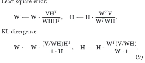
NMF algorithm starts with an initial estimate forWand

H, and performs an iterative optimization to minimize a given cost function. In [20], Lee and Seung introduce two updating algorithms using the least square error and the Kullback-Leibler (KL) divergence as the cost functions.

Least square error:

W←−W· VHT

WHHT, H←−H·

WT_V

WT_WH.

KL divergence:

W←−W·(V/WH)HT

1·H , H←−H·

WT_(V/WH)

W·1 .

(9)

Train MP-TFD

Audio signal x(t)

VM×N WM×r

Hr×N

NMF

Feature extraction

Fr×20

Fr×20

LDA classifier

{C}

Test Audio signal

x(t)

MP-TFD

VM×N

NMF

Feature extraction

LDA classifier

WM×r

Hr×N

1. Aircraft 2.Helicopter 3.Drum 4.Flute 5.Piano 6.Male 7.Female 8.Animal 9.Bird 10.Insect

Figure2: This block diagram represents the TFM quantification technique. In this approach, first the TFD (VK×N) of a signal (x(t)) is

estimated. Then a MD technique decomposes the estimated TF matrix intorbases components (WK×randHr×N). Finally, a discriminant

and representative feature vectorFis extracted from each decomposed component.

Wideband audio

TF modeling

TF parameter processing

Perceptual filtering Threshold

in quiet (TIQ)

Masking Quantizer

Media or channel

Figure3: Block diagram of ATFT audio coder.

We apply the TFM decomposition of the audio signals to perform environmental audio classification as is explained in

Section 4.2.

3. Audio Coding

In order to address the high demand for audio com-pression, over the years many compression methodologies were introduced to reduce the bit rates without sacrificing much of the audio quality. Since it is out of scope of this paper to cover all of the existing audio compression methodologies, the authors recommend the work of Painter and Spanias in [24] for a comprehensive review of most of the existing audio compression techniques. Audio signals are highly nonstationary in nature and the best way to analyze them is to use a joint TF approach. The presented coding methodology is based on ATFT and falls under the transform-like coder category. The usual methodology of a transform-based coding technique involves the following steps: (i) transforming the audio signal into frequency or TF-domain coefficients, (ii) processing the coefficients using psychoacoustic models and computing the audio masking thresholds, (iii) controlling the quantizer resolution using the masking thresholds, (iv) applying intelligent bit allocation schemes, and (v) enhancing the compression ratio with further lossless compression schemes. The ATFT-based coder nearly follows the above general transform coder methodology; however, unlike the existing techniques, the major part of the compression was achieved by exploiting the joint TF properties of the audio signals. The block

diagram of the ATFT coder is shown inFigure 3. The ATFT approach provides higher TF resolution than the existing TF techniques such as wavelets and wavelet packets [2]. This high-resolution sparse decomposition enables us to achieve a compact representation of the audio signal in the transform domain itself. Also, due to the adaptive nature of the ATFT, there was no need for signal segmentation.

Psychoacoustics were applied in a novel way on the TF decomposition parameters to achieve further compression. In most of the existing audio coding techniques the funda-mental decomposition components or building blocks are in the frequency domain with corresponding energy associated with them. This makes it much easier for them to adapt the conventional, well-modeled psychoacoustics techniques into their encoding schemes. On the other hand, in ATFT, the signal was modeled using TF functions which have a definite time and frequency resolution (i.e., each individual TF function is time limited and band limited), hence the existing psychoacoustics models need to be adapted to apply on the TF functions [25].

cannot be easily modeled since they do not have a definite TF localization or correlation with dictionary elements. Hence these noncoherent structures are broken down by the ATFT into smaller components to search for coherent structures. This process is repeated until the whole residue information is diluted across the whole TF dictionary [2]. From a compression point of view, it would be desirable to keep the number of iterations (M ≪ N), as low as possible and at the same time sufficient enough to model the audio signal without introducing perceptual distortions. Considering this requirement, an adaptive limit has to be set for controlling the number of iterations. The energy capture rate (signal energy capture rate per iteration) could be used to achieve this. By monitoring the cumulative energy capture over iterations we could set a limit to stop the decomposition when a particular amount of signal energy was captured. The minimum number of iterations required to model an audio signal without introducing perceptual distortions depends on the signal composition and the length of the signal. In theory, due to the adaptive nature of the ATFT decomposition, it is not necessary to segment the signals. However, due to the computational resource limitations (Pentium III, 933 MHZ with 1 GB RAM), we decomposed the audio signals in 5 s durations. The larger the duration decomposed, the more efficient is the ATFT modeling. This is because if the signal is not sufficiently long, we cannot efficiently utilise longer TF functions (highest possible scale) to approximate the signal. As the longer TF functions cover larger signal segments and also capture more signal energy in the initial iterations, they help to reduce the total number of TF functions required to model an audio signal. Each TF function has a definite time and frequency localization, which means all the information about the occurrences of each of the TF functions in time and frequency of the signal is available. This flexibility helps us later in our processing to group the TF functions corresponding to any short time segments of the audio signal for computing the psychoacoustic thresholds. In other words, the complete length of the audio signal can be first decomposed into TF functions and later the TF functions corresponding to any short time segment of the signal can be grouped together. In comparison, most of the DCT- and MDCT-based existing techniques have to segment the signals into time frames and process them sequentially. This is needed to account for the non-stationarity associated with the audio signals and also to maintain a low signal delay in encoding and decoding.

In the presented technique for a signal duration of 5 s, the decomposition limit was set to be the number of iterations (Mx) needed to capture 99.5% of the signal energy or to a

maximum of 10,000 iterations and is given by

Mx=

⎧ ⎪ ⎪ ⎪ ⎨ ⎪ ⎪ ⎪ ⎩

M, ifM <10000, .995=

M−1

n=0 Rnx,gγn 2

_∞

−∞|x(t)|2dt

,

10000, otherwise.

(10)

For a signal with less noncoherent structures, 99.5% of signal energy could be modeled with a lower number of TF

functions than a signal with more noncoherent structures. In most cases a 99.5% of energy capture nearly characterises the audio signal completely. The upper limit of the iterations is fixed to 10,000 iterations to reduce the computational load.

Figure 4demonstrates the number of TF functions needed for a sample audio signal. In the figure, the lower panel shows the energy capture curve for the sample audio signal in the top panel with number of TF functions in theX-axis and the normalised energy in theY-axis. On average, it was observed that 6000 TF functions are needed to represent a signal of 5 s duration sampled at 44.1 kHz.

3.2. Implementation of Psychoacoustics. In the conventional coding methods, the signal is segmented into short time segments and transformed into frequency domain coeffi -cients. These individual frequency components are used to compute the psychoacoustic masking thresholds and accordingly their quantization resolutions are controlled. In contrast, in our approach we computed the psychoa-coustic masking properties of individual TF functions and used them to decide whether a TF function with certain energy was perceptually relevant or not based on its time occurrence with other TF functions. TF functions are the basic components of the presented technique and each TF function has a certain time and frequency support in the TF plane. So their psychoacoustical properties have to be studied by taking them as a whole to arrive at a suitable psychoacoustical model. More details on the implementation of psychoacoustics is covered in [25,26].

3.3. Quantization. Most of the existing transform-based coders rely on controlling the quantizer resolution based on psychoacoustic thresholds to achieve compression. Unlike this, the presented technique achieves a major part of the compression in the transformation itself followed by perceptual filtering. That is, when the number of iterations

M needed to model a signal is very low compared to the length of the signal, we just needM×Lbits. WhereLis the number of bits needed to quantize the 5 TF parameters that represent a TF function. Hence, we limited our research work to scalar quantizers as the focus of the research mainly lies on the TF transformation block and the psychoacoustics block rather than the usual sub-blocks of the data compression application.

As explained earlier each of the five parameters Energy (an), Center frequency (fn), Time position (pn), Octave

(sn), and Phase (φn) are needed to represent a TF function

and thereby the signal itself. These five parameters were to be quantized in such a way that the quantization error introduced was imperceptible while, at the same time, obtaining good compression. Each of the five parameters has different characteristics and dynamic range. After careful analysis of them the following bit allocations were made. In arriving at the final bit allocations informal Mean Opinions Score (MOS) tests were conducted to compare the quality of the audio samples before and after quantization stage.

−0.2

−0.1 0 0.1 0.2

A

m

plitude

(a.u.)

0.2 0.4 0.6 0.8 1 1.2 1.4 1.6 1.8 2 2.2

×105 Time samples

Sample signal

(a)

0 0.2 0.4 0.6 0.8 1

×10−3

Energ

y

(a.u.)

0 1000 2000 3000 4000 5000 6000 7000 8000 9000 10000 Number of TF functions

Energy curve

99.5% of the signal energy

(b)

Figure4: Energy cutoffof the sample signal in panel 1. a.u.: arbitrary units.

noise in the reconstructed signal. The final form of data for

MTF functions will contain the following.

(i) Energy parameter (Log companded)=M∗12 bits. (ii) Time position parameter=M∗15 bits.

(iii) Center frequency parameter=M∗13 bits. (iv) Phase parameter=M∗10 bits.

(v) Octave parameter=M∗4 bits.

The sum of all the above (= 54 ∗ M bits) will be the total number of bits transmitted or stored representing an audio segment of duration 5 s. The energy parameter after log companding was observed to be a very smooth curve. Fitting a curve to the energy parameter further reduces the bit rate [25, 26]. With just a simple scalar quantizer and curve fitting of the energy parameter, the presented coder achieves high-compression ratios. Although a scalar quantizer was used to reduce the computational complexity of the presented coder, sophisticated vector quantization techniques can be easily incorporated to further increase the coding efficiency. The 5 parameters of the TF function can be treated as one vector and accordingly quantized using predefined codebooks. Once the vector is quantized, only the index of the codebook needs to be transmitted for each set of TF parameters resulting in a large reduction of the total number of bits. However designing the codebooks would be challenging as the dynamic ranges of the 5 TF parameters are drastically different. Apart from reducing the number of total bits, the quantization stage can also be utilized to control the bit rates suitable for CBR (Constant Bit Rate) applications.

3.4. Compression Ratios. Compression ratios achieved by the presented coder were computed for eight sample wideband audio signals (of 5 s duration) as described below. These eight sample signals (namely, ACDC, DEFLE, ENYA, HARP, HARPSICHORD, PIANO, TUBULARBELL, and VISIT) were representatives of wide range of music types.

(i) As explained earlier, the total number of bits needed to represent each TF function is 54.

(ii) The energy parameter is curve fitted and only the first 150 points in addition to the curve fitted point need to be coded.

(iii) So the total number of bits needed forM iterations for a 5 s duration of the signal isTB1 =(M∗42) +

((150 +C)∗12), whereC is the number of curve fitted points, andM is the number of perceptually important functions.

(iv) The total number of bits needed for a CD quality 16 bit PCM technique for a 5 s duration of the signal sampled at 44100 Hz is TB2 = 44100∗5∗16 =

3, 528, 000.

(v) The compression ratio can be expressed as the ratio of number of bits needed by the presented coder to the number of bits needed by the CD quality 16 bit PCM technique for the same length of the signal, that is,

Compression ratio=TB2 TB1

. (11)

The presented coder is based on an adaptive signal trans-formation technique, that is, the content of the signal and the dictionary of basis functions used to model the signal play an important role in determining how compact a signal can be represented (compressed). Hence, VBR (Variable Bit Rate) is the best way to present the performance benefit of using an adaptive decomposition approach. The inherent variability introduced in the number of TF functions required to model a signal and thereby the compression is one of the highlights of using ATFT. Although VBR would be more appropriate to present the performance benefit of the presented coder, CBR mode has its own advantages when using with applications that demand network transmissions over constant bitrate channels with limited delays. The presented coder can also be used in CBR mode by fixing the number of TF functions used for representing signal segments, however due to the signal adaptive nature of the presented coder this would compromise the quality at instances where signal segments demand a higher number of TF functions for perceptually lossless reproduction. Hence we choose to present the results of the presented coder using only the VBR mode.

We compared the presented coder with two existing popular and state-of-the-art audio coders, namely, MP3 (MPEG 1 layer 3) and MPEG-4 AAC/HE-AAC. Advanced audio coding (AAC) is the current industrial standard which was initially developed for multichannel surround signals (MPEG-2 AAC [27]). As there are ample studies in the literature [27–32] available for both MP3 and MPEG-2/4 AAC more details about these techniques are not provided in this paper. The average bit rates were used to calculate the compression ratio achieved by MP3 and MPEG-4 AAC as described below.

(i) Bitrate for a CD quality 16 bit PCM technique for 1 s stereo signal is given byTB3=2∗44100∗16.

(ii) The average bit rate/s achieved by (MP3 or MPEG-4 AAC) in VBR mode=TB4.

(iii) Compression ratio achieved by (MP3 or MPEG-4 AAC)=TB3/TB4.

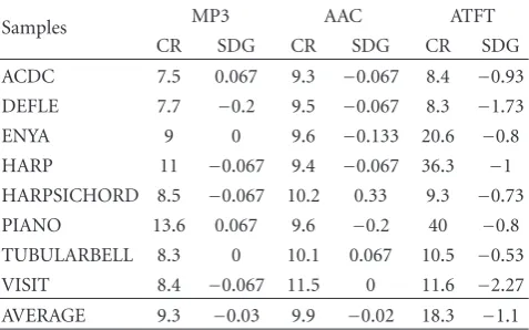
The 2nd, 4th and 6th columns of Table 1 show the compression ratio (CR) achieved by the MP3, MPEG-4 AAC and the presented ATFT coders for the set of 8 sample audio files. It is evident from the table that the presented coder has better compression ratios than MP3. When comparing with MPEG-4 AAC, 5 out of 8 signals are either comparable or have better compression ratios than the MPEG-4 AAC. It is noteworthy to mention that for slow music (classical type) the ATFT coder provides 3 to 4 times better comparison than MPEG-4 AAC or MP3.

The compression ratio alone cannot be used to evaluate an audio coder. The compressed audio signals has to undergo a subjective evaluation to compare the quality achieved with respect to the original signal. The combination of the subjective rating and the compression ratio will provide a true evaluation of the coder performance.

Before performing the subjective evaluation, the signal has to be reconstructed. The reconstruction process is a

Table1: Compression ratio (CR) and subjective difference grades (SDGs). MP3: Moving Picture Experts Group I Layer 3, MPEG-4 AAC: Moving Picture Experts Group 4 Advanced Audio Coding, VBR Main LTP profile, and ATFT: Adaptive Time-Frequency Transform.

Samples MP3 AAC ATFT

CR SDG CR SDG CR SDG

ACDC 7.5 0.067 9.3 −0.067 8.4 −0.93

DEFLE 7.7 −0.2 9.5 −0.067 8.3 −1.73

ENYA 9 0 9.6 −0.133 20.6 −0.8 HARP 11 −0.067 9.4 −0.067 36.3 −1

HARPSICHORD 8.5 −0.067 10.2 0.33 9.3 −0.73

PIANO 13.6 0.067 9.6 −0.2 40 −0.8

TUBULARBELL 8.3 0 10.1 0.067 10.5 −0.53

VISIT 8.4 −0.067 11.5 0 11.6 −2.27

AVERAGE 9.3 −0.03 9.9 −0.02 18.3 −1.1

straightforward process of linearly adding all the TF func-tions with their corresponding five TF parameters. In order to do that, first the TF parameters modified for reducing the bit rates have to be expanded back to their original forms. The log compressed energy curve was log expanded after recovering back all the curve points using interpolation on the equally placed 50 length points. The energy curve was multiplied with the normalization factor to bring the energy parameter as it was during the decomposition of the signal. The restored parameters (Energy, Time-position, Center frequency, Phase and Octave) were fed to the ATFT algorithm to reconstruct the signal. The reconstructed signal was then smoothed using a 3rd-order Savitzky-Golay [33] filter and saved in a playable format.

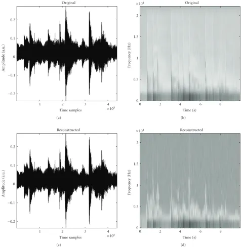
Figure 5demonstrates a sample signal (/“HARP”/) and its reconstructed version and the corresponding spectro-grams. It can be clearly observed from the reconstructed signal spectrogram compared with the original signal spec-trogram, how accurately the ATFT technique has filtered out the irrelevant components from the signal (evident fromTable 1—(/“HARP”/)—high-compression ratio versus acceptable quality). The accuracy in adaptive filtering of the irrelevant components is made possible by the TF resolution provided by the ATFT algorithm.

−0.2

−0.1 0 0.1 0.2

A

m

plitude

(a.u.)

1 2 3 4

×105 Time samples

Original

(a)

0 0.5 1 1.5 2

×104

Fre

q

u

en

cy

(H

z)

0 2 4 6 8

Time (s) Original

(b)

−0.2

−0.1 0 0.1 0.2

A

m

plitude

(a.u.)

1 2 3 4

×105 Time samples

Reconstructed

(c)

0 0.5 1 1.5 2

×104

Fre

q

u

en

cy

(H

z)

0 2 4 6 8

Time (s) Reconstructed

(d)

Figure5: Example of a sample original (/“HARP”/) and the reconstructed signal with their respective spectrograms.X-axes for the original

and reconstructed signal are in time samples, andX-axes for the spectrogram of the original and the reconstructed signal are in equivalent

time in seconds. Note that the sampling frequency=44.1 kHz. au: arbitrary units.

Difference Grade (SDG) [24] was computed by subtracting the absolute score assigned to the hidden reference audio signal from the absolute score assigned to the compressed audio signal. It is given by

SDG=Grade{compressed}−Grade{reference}. (12)

Accordingly the scale of SDG will range from (−4 to 0) with the following interpretation: (−4): Unsatisfactory (or) Very Annoying, (−3): Poor (or) Annoying, (−2): Fair

(or) Slightly annoying, (−1): Good (or) Perceptible but not annoying, and (0): Excellent (or) Imperceptible. Fifteen listeners (randomly selected) participated in the MOS studies and evaluated all the 3 audio coders (MP3, AAC and ATFT in VBR mode). The average SDG was computed for each of the audio sample. The 3rd, 5th and 7th columns of the

3.6. Results and Discussion. The compression ratios (CRs) and the SDG for all three coders (MP3, AAC and ATFT) are shown inTable 1. All the coders were tested in the VBR mode. For the presented technique, VBR was the best way to present the performance benefit of using an adaptive decomposition approach. In ATFT, the type of the signal and the characteristics of the TF functions (type of dictionary) control the number of transformation parameters required to approximate the signal and thereby the compression ratio. The inherent variability introduced in the number of TF functions required to model a signal is one of the highlights of using ATFT. Hence we choose to present comparison of the coders in the VBR mode.

The results show that the MP3 and AAC coders per-form well with excellent SDG scores (Imperceptible) at a compression ratio around 10. The presented coder does not perform well with all of the eight samples. Out of the 8 samples, 6 samples have an SDG between −0.53 to

−1 (Imperceptible—perceptible but not annoying) and 2 samples have SDG below −1. Out of the 6 samples with SDGs between (−0.53 and−1), 3 samples (ENYA, HARP and PIANO) have compression ratios 2 to 4 times higher than MP3 and AAC and 3 samples (ACDC, HARPSICHORD and TUBULARBELL) have comparable compression ratios with moderate SDGs.

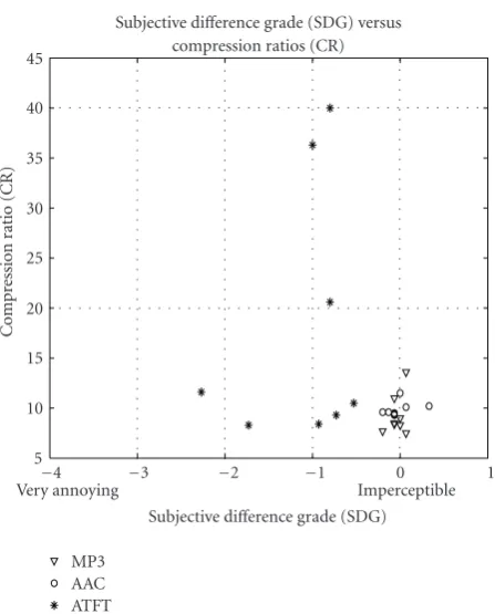
Figure 6 shows the comparison of all three coders by plotting the samples with their SDGs in X-axis and compression ratios in theY-axis. If we can virtually divide this plot in segments of SDGs (horizontally) and the compression ratios (vertically), then the ideal desirable coder performance should be in the right top corner of the plot (high-compression ratios and excellent SDG scores). This is followed next by the right bottom corner (low-compression ratios and excellent SDG scores) and so on as we move from right to left in the plot. Here the terms “Low”- and “High”-compression ratios are used in a relative sense based on the compression ratios achieved by all the 3 coders in this study. From the plot it can be seen that MP3 and AAC coders occupy the right bottom corner, whereas the samples from ATFT coder are spread over. As mentioned earlier 3 out the 8 samples of the ATFT coder occupy the right top corner only with moderate SDGs that are much less than the MP3 and the AAC. 3 out of the remaining 5 samples of the ATFT coder occupy the right bottom corner, again with only moderate SDGs that are less than MP3 and AAC. The remaining 2 samples perform the worst occupying the left bottom corner. We analyzed the poorly performing ATFT coded signals DEFLE and VISIT. DEFLE is a rapidly varying rock-like signal with minimal voice components and VISIT is a signal with dominant voice components. We observed that the symmetrical and smooth Gaussian dictionary used in this study does not model the transients well, which are the main features of all rapidly varying signals like DEFLE. This inefficient modeling of transients by the symmetrical Gaussian TF functions resulted in the poor SDG for the DEFLE. A more appropriate dictionary would be a damped sinusoids dictionary [35] which can better model the transient-like decaying structures in audio signals. However a single dictionary alone may not be sufficient to model

5 10 15 20 25 30 35 40 45

C

o

mpr

ession

ra

tio

(CR)

−4 −3 −2 −1 0 1

Very annoying Imperceptible

Subjective di_fference grade (SDG) Subjective difference grade (SDG) versus

compression ratios (CR)

MP3 AAC ATFT

Figure6: Subjective Difference Grade (SDG) versus Compression ratios (CRs).

all types of signal structures. The second signal VISIT has significant amount(s) of voice components. Even though the main voice components are modeled well by the ATFT, the noise-like hissing and shrilling sounds (noncoherent structures) could not be modeled within the decomposition limit of 10,000 iterations. These hissing and shrilling sounds actually add to the pleasantness of the music. Any distortion in them is easily perceived which could have reduced the SDG of the signal to the lowest of the group −2.27. The poor performances with the two audio sample cases could be addressed by using a hybrid dictionary of TF functions and residue coding the noncoherent structures separately. However this would increase the computational complexity of the coder and reduce the compression ratios.

From the results presented for the ATFT coder, the signal adaptive performance of the coder for a specific TF dictionary is evident, that is, with a Gaussian TF dictionary the coder performed moderately well for slow-varying classical signals than fast slow-varying rock-like signals. In other words the ATFT algorithm demonstrated notable differences in the decomposition patterns of classical and rock-like signals. This is a valid clue and a motivating factor that these differences in the decomposition patterns if quantified using TF decomposition parameters could be used as discriminating features for classifying audio signals. We apply this hypothesis in extracting TF features for classifying audio signals for a content-based audio retrieval application as will be explained inSection 4.

3.7. Summary of Steps Involved in Implementing ATFT Audio Coder

Step 1 (ATFT algorithm and TF dictionaries). Existing implementation of Matching Pursuits can be adapted for the purposes; (1) LastWave (http://www.cmap.polytechnique.fr/

∼bacry/LastWave/), (2) Matching Pursuit Package (MPP) (ftp://cs.nyu.edu/pub/wave/software/mpp.tar.Z), and (3) Matching Pursuit ToolKit (MPTK) [36].

Step 2 (Control decomposition). The number of TF func-tions required to model a fixed segment of audio signal can be arrived using similar criteria described inSection 3.1.

Step 3 (Perceptual Filtering). The TF functions obtained fromStep 2can be further filtered using the psychoacoustics thresholds discussed inSection 3.2.

Step 4 (Quantization). The simple quantization scheme presented in Section 3.3can be used for bit allocation or advanced vector quantization methods can also be explored.

Step 5 (Lossless schemes). Further lossless schemes can be applied to the quantized TF parameters to further increase the compression ratio.

4. Audio Classification

Audio feature extraction plays an important role in analyzing and characterizing audio content. Auditory scene analysis, content-based retrieval, indexing, and fingerprinting of audio are few of the applications that require efficient feature extraction. The general methodology of audio classification involves extracting discriminatory features from the audio data and feeding them to a pattern classifier. Different approaches and various kinds of audio features were pro-posed with varying success rates. Audio feature extraction serves as the basis for a wide range of applications in the areas of speech processing [37], multimedia data management and distribution [38–41], security [42], biometrics and bioacous-tics [43]. The features can be extracted either directly from the time-domain signal or from a transformation domain depending upon the choice of the signal analysis approach. Some of the audio features that have been successfully

Audio

signal Adaptive signal decomposition

Feature extraction

Linear discriminant

analysis

Rock Classical Country Folk Jazz Pop

Figure 7: Block diagram of the proposed music classification scheme.

used for audio classification include mel frequency cepstral coefficients (MFCCs) [40, 41], spectral similarity [44], timbral texture [41], band periodicity [38], LPCC (Linear Prediction Coefficient-derived cepstral coefficients) [45], zero crossing rate [38,45], MPEG-7 descriptors [46], entropy [12], and octaves [39]. Few techniques generate a pattern from the features and use it for classification by the degree of correlation. Few other techniques use the numerical values of the features coupled to statistical classification methods.

4.1. Music Classification. In this section, we present a content-based audio retrieval application employing audio classification and explain the generic steps involved in performing successful audio classification. The simplest of all retrieval techniques is the text-based searching where the information about the multimedia data is stored with the data file. However the success of these type of text-based searches depend on how well they are text indexed by the author and they do not provide any information on the real content of the data. To make the retrieval system automated, efficient, and intelligent, content-based retrieval techniques were introduced. The presented work focuses on one such way for automatic classification of audio signals for retrieval purposes. The block diagram of the proposed technique is shown inFigure 7.

In content-based retrieval systems, audio data is ana-lyzed, and discriminatory features are extracted. The selec-tion of features depends on the domain of analysis and the perceptual characteristics of the audio signals under consideration. These features are used to generate subspaces dividing the audio signal types to fit in one of the subspaces. The division of subspaces and the level of classification vary from technique to technique. When a query is placed the similarity of the query is checked with all subspaces and the audio signals from the highly correlated subspace is returned as the result. The classification accuracy, and the discriminatory power of the features extracted determine the success of such retrieval systems.

−0.2

−0.1 0 0.1 0.2

A

m

plitude

(a.u.)

0.2 0.4 0.6 0.8 1 1.2 1.4 1.6 1.8 2 2.2

×105 Time samples

Sample music signal

(a)

−0.2

−0.1 0 0.1 0.2

A

m

plitude

(a.u.)

0.2 0.4 0.6 0.8 1 1.2 1.4 1.6 1.8 2 2.2

×105 Time samples

Reconstructed signal with 10 TF functions

Octave or scale

(b)

Figure8: A sample music signal, and its reconstructed version with 10 TF functions.

multiple features are used for classification, in the proposed technique, only one TF decomposition parameter is used to generate a feature set from different frequency bands for classification. Due to its strong discriminatory power, just one TF decomposition parameter is sufficient enough for accurate classification of music into six groups.

4.1.1. Audio Database. A database consisting of 170 audio signals was used in the proposed technique. Each audio signal is a segment of 5 s duration extracted from individual original CD music tracks (wide band audio at 44100 samples/second) and no more than one audio signal (5 s duration) was extracted from the same music track. The 170 audio signals consist of 24 rock, 35 classical, 31 country, 21 jazz, 34 folk, and 25 pop signals. As all signals of the database were extracted from commercial CD music tracks, they exhibited all the required characteristics of their respective music genre, such as guitars, drumbeats, vocal, and piano. The signal duration of 5 s was arrived at using the rationale that the longer the audio signal analyzed, the better the extracted feature which exhibits more accurate music characteristics. As the ATFT algorithm is adaptive and does not need any segmentation, theoretically there is no limit for the signal length. However considering the hardware (Pentium III @ 933 MHz and 1.5 GB RAM) limitations of the processing facility, we used 5 s duration samples. In the proposed technique first all the signals were chosen between 15 s to 20 s of the original music tracks. Later by inspection those segments, which were inappropriately selected were replaced by segments (5 s duration) at random locations of the original music track in such way their music genre is exhibited.

4.1.2. Feature Extraction. All the signals were decomposed using the ATFT algorithm. The decomposition parameters provided by the ATFT algorithm were analyzed, and the octave sn parameter was observed to contain significant

information on different types of music signals. In the decomposition process, the octave or scaling parameter is decided by the adaptive window duration of the Gaussian function that is used in the best possible approximation of the local signal structures. Higher octaves correspond to longer window durations and the lower octaves correspond to shorter window duration. In other words combinations of these octaves represent the envelope of the signal. The envelope (temporal structures) [47] of an audio signal provides valid clues such as rhythmic structure [41], indirect pitch content [41], phonetic composition [48], tonal and transient contributions. Figure 8 demonstrates a sample piece of a music signal and its reconstructed version using 10 TF functions. The relation between the octave parameter and the envelope of the signal is clearly seen. Based on the composition of different structures in a signal, the octave mapping or distribution varies significantly. For example, more lower-order octaves are needed for signals containing lot of transient-like structures and on the other hand more higher-order octaves are needed for signal containing rhythmic tonal components. As an illustration, fromFigure 9

0 0.5 1

Fre

q

u

en

cy

0 2 4 6 8 10

Time Signal 1

(a)

0 0.5 1

Fre

q

u

en

cy

0 2 4 6 8 10

Time Signal 2

(b)

0 0.5 1

N

o

rm

alised

dist

ribution

1 2 3 4 5 6 7 8 9 10 11 12 13 Octaves

Octave distribution signal 1

(c)

0 0.5 1

N

o

rm

alised

dist

ribution

1 2 3 4 5 6 7 8 9 10 11 12 13 Octaves

Octave distribution signal 2

(d)

0 0.5 1

Fre

q

u

en

cy

0 2 4 6 8 10

Time Signal 3

(e)

0 0.5 1

Fre

q

u

en

cy

0 2 4 6 8 10

Time Signal 4

(f)

0 0.5 1

N

o

rm

alised

dist

ribution

1 2 3 4 5 6 7 8 9 10 11 12 13 Octaves

Octave distribution signal 3

(g)

0 0.5 1

N

o

rm

alised

dist

ribution

1 2 3 4 5 6 7 8 9 10 11 12 13 Octaves

Octave distribution signal 4

(h)

0 100 200 D ist ri but ion of octa ve s

1 2 3 4 5 6 7 8 9 10 11 12 13 14 Octaves

Rock sample signal

Frequency band (10–20 kHz)

(a) 0 500 1000 D ist ri but ion of octa ve s

1 2 3 4 5 6 7 8 9 10 11 12 13 14 Octaves

Rock sample signal Frequency band (5–10 kHz)

(b) 0 500 1000 D ist ri but ion of octa ve s

1 2 3 4 5 6 7 8 9 10 11 12 13 14 Octaves

Rock sample signal Frequency band (0–5 kHz)

(c)

Figure10: Octave distribution over three frequency bands for a rock signal.

To further improve the discriminatory power of this parameter the distribution of this parameter is grouped into three frequency bands 0–5 kHz, 5–10 kHz, and 10–20 kHz. This is done since analyzing the audio signals in subbands will provide more precise information about their audio characteristics [49]. The bounds for frequency bands were arrived considering the fact that most of the audio content lies well within 10 kHz range so this band needs to be looked more in detail hence broken further into 0–5 kHz and 5 kHz to 10 kHz and the remaining as one band between 10 kHz to 20 kHz. By this frequency division we get an indirect measure of signal envelope contribution from each frequency band. From Figure 9even though we see difference in the distribution of octaves between rock-like and classical music, it becomes more evident when the distribution is divided into three frequency bands as shown for a sample rock and a classical signal in Figures 10 and 11. Dividing the octave distribution into frequency bands basically reveal the pattern in which the temporal structures occur over the range of frequencies. As music is the combination of different temporal structures with different frequencies occurring at same or different time instants, each type of music exhibit a unique average pattern. Based on the subtle differences between patterns to be detected, the division of octave distribution over fine frequency intervals and the dimension of the feature set can be controlled.

0 5 10 15 20 D ist ri but ion of octa ve s

1 2 3 4 5 6 7 8 9 10 11 12 13 14 Octaves

Classical sample signal Frequency band (10–20 kHz)

(a) 0 5 10 15 20 D ist ri but ion of octa ve s

1 2 3 4 5 6 7 8 9 10 11 12 13 14 Octaves

Classical sample signal Frequency band (5–10 kHz)

(b) 0 5 10 15 20

×102

D ist ri but ion of octa ve s

1 2 3 4 5 6 7 8 9 10 11 12 13 14 Octaves

Classical sample signal Frequency band (0–5 kHz)

(c)

Figure11: Octave distribution over three frequency bands for a classical signal.

After decomposing all the audio signals using ATFT, the TF functions were grouped into three frequency bands based on their center frequencies fn. Then the distribution of each

of the 14 octave parametersnvalues were calculated over the

3 frequency bands to get a total of 14×3 = 42 different distribution values. All these 42 values of each audio segment were used as a feature set for classification. As an illustration, in Figures 10 and 11 the X-axis represents the 14 octave parameters and theY-axis represents the distribution of the octave parameters over three frequency bands for 10,000 iterations. Each of the distribution value forms one of 42 elements in the feature set.

4.1.3. Pattern Classification. The motivation for the pattern classification is to automatically group audio signals of same characteristics using the discriminatory features derived as explained in previous subsection.

Pattern classification was carried out by linear dis-criminant analysis (LDA)-based classifier using the SPSS software [50]. In discriminant analysis, the feature vector derived as explained above were transformed into canonical discriminant functions such as

Table 2: Classification results. Method: Regular: linear discrim-inant analysis, Cross-validated: linear discrimdiscrim-inant analysis with leave-one-out method, CA%: Classification Accuracy Rate, Gr: Groups, Ro: Rock, Cl: Classical, Co: Country, Ja: Jazz, Fo: Folk and Po: Pop.

Method Gr Ro Cl Co Ja Fo Po CA%

Regular Ro 24 0 0 0 0 0 100

Cl 0 35 0 0 0 0 100

Co 0 0 31 0 0 0 100

Ja 0 2 0 19 0 0 90.5

Fo 1 0 0 1 32 0 94.1

Po 0 0 0 0 0 25 100

Overall 97.6

Cross- Ro 23 0 1 0 0 0 95.8

Validated Cl 0 34 0 1 0 0 97.1

Co 1 0 29 0 1 0 93.5

Ja 0 3 0 18 0 0 85.7

Fo 1 1 0 2 30 0 88.2

Po 2 0 2 0 0 21 84

Overall 91.2

where{u}is the set of features,{b}andaare the coefficients and constant, respectively. The feature dimension q repre-sents the number of features used in the analysis. Using the discriminant scores and the prior probability values of each group, the posterior probabilities of each sample occurring in each of the groups were computed. The sample was then assigned to the group with the highest posterior probability [50].

The classification accuracy was estimated using the leave-one-out method which is known to provide a least bias estimate [51]. In the leave-one-out method, one sample is excluded from the dataset and the classifier is trained with the remaining samples. Then the excluded signal is used as the test data and the classification accuracy is determined. This is repeated for all samples of the dataset. Since each signal is excluded from the training set in turn, the independence between the test and the training set are maintained.

4.1.4. Results and Discussion. A database of 170 audio signals consisting of 24 rock, 35 classical, 31 country, 21 jazz, 34 folk and 25 pop each of 5 s duration was used. All the 170 audio signals were decomposed and the feature set of 42 octave distribution values were extracted. The extracted feature sets for the entire 170 signals were fed to the classifier based on LDA. Six-group classification was performed (rock, classical, country, jazz, folk and pop). Table 2 shows the confusion matrices for different classification procedures. An overall classification accuracy of 97.6% is achieved by the regular LDA method and 91.2% with the leave-one-out-based LDA method. In the regular LDA method, all the 24 rock, 35 classical, 31 country, and 25 pop were correctly classified with 100% classification accuracy. Two out of 21 jazz and 2 out of 34 folk signals were misclassified with a correct classification accuracy of 90.5% and 94.1%, respectively. The classification accuracy of 91.2% with the leave-one-out

−8

−6

−4

−2 0 2 4 6

Fu

n

ct

io

n

2

−10 −8 −6 −4 −2 0 2 4 6 Function 1

Rock Classical Country

Folk Jazz Pop

Figure 12: All-groups scatter plot with the first two canonical discriminant functions.

method proves the robustness of the proposed technique and independence of the achieved results irrespective of the dataset size.Figure 12shows the all-groups scatter plot with the first two canonical discriminant functions. One can clearly observe the significant separation between the group spaces explaining the high-discriminatory power of the feature set based on the octave distribution.

The misclassified signals were analyzed but could not identify a clear auditory clue to why they were misclassified. However their differences are observed in the feature set. Considering the known fact that no music genre has clear hard line boundaries and the perceptual boundaries are often subjective (e.g., rock and pop often have overlaps and likewise jazz and classical too have overlaps), we may attribute the classification error of these signals on the natural overlap of the music genre and the amount of knowledge imparted to the classifier with the given database. In this section, we have covered details involved in a simple audio classification task using a time-frequency approach. The high-classification accuracies achieved by the proposed technique clearly demonstrate the potential of a true nonstationary tool in the form of a joint TF approach for audio classification. More interestingly a single TF decomposition parameter is used for feature extraction proving the high-discriminatory power provided by TF approach compared to the existing techniques.

the content of multimedia. Therefore, developing audio clas-sification techniques that better characterize audio signals plays an essential role in many multimedia implications such as (a) multimedia indexing and retrieval, and (b) auditory scene analysis.

4.2.1. Audio Database. The lack of a common dataset does not allow researchers to compare the performance of different audio classification methodologies in a fair manner. Some literatures report an impressive accuracy rate, but they use only a small number of classes and/or a small dataset in their evaluations. The number of classes used in literature varies from study to study. For example, in [52], the authors use two classes (i.e., speech and music) while audio content analysis at Microsoft research [53] uses four audio classes (i.e., speech, music, environment sound, and silence). Free-man et al. [54] uses four classes of speech (i.e., babble, traffic noise, typing, and white noise) while the authors in [55] use 14 different environmental scenes (i.e., inside restaurants, playground, street traffic, train passing, inside moving vehi-cles, inside casinos, street with police car siren, street with ambulance siren, nature daytime, nature nighttime, Ocean waves, running water, rain, and thunder). In this work we use an environmental audio dataset that was developed and compiled in our signal analysis research (SAR) group at Ryer-son University. This database consists of 192 audio signals of 5 s duration each with a sampling rate of 22.05 kHz and a resolution of 16 bits/sample. It is designed to have 10 diff er-ent classes including 20 aircraft, 17 helicopters, 20 drums, 15 flutes, 20 pianos, 20 animals, 20 birds and 20 insects, and the speech of 20 males and 20 females. Most of the music samples were collected from the Internet and suitably processed to have uniform sampling frequency and duration.

4.2.2. Feature Extraction. All signals were decomposed using the TFM decomposition method. First, we perform the MP-TFD on 3 s duration of each signal, and construct the TFM of each signal. Next, NMF with decomposition order of 15 (r = 15) is performed on each MP-TF matrix, and 15 base vectors and 15 coefficient vectors are extracted for each signal. Figures13and14show the decomposition vectors of an aircraft and a piano signal, respectively.

20 features are extracted from each decomposed base and coefficient vector. 13 of the features are the first 13 MFCC of each base vector, and the next six features are

Sh, Sw, Dh, Dw, MOh, MOw, and MP. These features are

explained as follows:

(a)ShiandSwiare the sparsity of coefficient and base

vec-tors, respectively. This feature helps to distinguish between transient and continuous components. Several sparseness measures have been proposed and used in the literature. We propose a sparsity function as follows

Shi=Log10 √

N−N n=1hi(n)

/Nn=1h2i(n)

√

N−1 ,

(14)

Swi=Log10 √

K−K k=1wi(k)

/Kk=1w2i(k)

√

K−1 .

(15)

The sparsity is zero if and only if a vector contains a single nonzero component, and is negative infinity if and only if all the components are equal. The sparsity measure in (15) has been used for applications such as NMF matrix decompo-sition with more part-based properties [56]; however, it has never been used for feature extraction application.

(b)Dh andDwrepresent the discontinuities and abrupt

changes in each vector. These features are calculated as follows:

Dhi=Log10

N−1

n=1 hi(n)2,

Dwi=Log10

K−1

k=1 wi(k)2,

(16)

where hi and wi are derivatives of coefficient and base

vectors, respectively

hi(n)=hi(n+ 1)−hi(n), n=1,. . .,N−1,

wi(k)=wi(k+ 1)−wi(k), k=1,. . .,K−1.

(17)

(c) MOh and MOw represent the temporal and spectral

moments, respectively. Our observation showed that the temporal and spectral spread of the TF energy are discrim-inant characteristics for different audio groups. To quantify this property, we extract the second moment around the mean of each coefficient and base vectors as follows:

MOhi=Log10

N

n=1

n−μhi 2

hi(n),

MOwi =Log10

K

k=1

k−μwi 2

wi(k),

(18)

whereμhi andμwi are the mean of the coefficient and base

vectori, respectively.

(d) MP is the Matching Pursuit Feature. Using M

iterations of MP, we project an audio signal into a linear combination of Gaussian functionsgγn(t) as shown in (3).

The amount of signal energy that is projected at each iteration depends on the signal structure. The signal with coherent structure needs less number of iterations, while noncoherent structured signals take more iterations to get decomposed. In order to calculate MP feature in a way that it discriminates coherent signals from noncoherent ones, and it is independent from the signal’s energy, we calculate sum of the normalized projected energy per iteration as MP. The MP feature for piano and aircraft signals is calculated as 2.9 and 10.6, respectively. As it is expected, MP feature is high for the noncoherent segment (aircraft), and low for the coherent segment (piano).