On the Hardness of Learning With Errors with Binary Secrets
Daniele Micciancio∗ October 14, 2018
Abstract
We give a simple proof that the decisional Learning With Errors (LWE) problem with binary secrets (and an arbitrary polynomial number of samples) is at least as hard as the standard LWE problem (with unrestricted, uniformly random secrets, and a bounded, quasi-linear number of samples). This proves that the binary-secret LWE distribution is pseudorandom, under standard worst-case complexity assumptions on lattice problems. Our results are similar to those proved by (Brakerski, Langlois, Peikert, Regev and Stehl´e, STOC 2013), but provide a shorter, more direct proof, and a small improvement in the noise growth of the reduction.
1
Introduction
The Learning With Errors (LWE) problem [21, 22] plays a central role in lattice cryptography, its secure instantiation, and its most advanced applications. The usefulness of LWE in cryptography is due in large part to its pseudorandomness properties, captured by the standard decisional LWE problem defined as follows. An LWE instance is described by a matrixA∈Zm×n
q (chosen uniformly
at random) and a vectorb∈Zmq which may be chosen either uniformly at random, or asb=As+e
(modq), where s ∈Zn
q is a random secret and e∈ Zm is a “small” error vector, typically chosen
with independent discrete Gaussian entries of standard deviation σ≈√n. The (Decisional) LWE problem asks to distinguish between these two cases.
Several variants of LWE exist in the literature, depending on how s and e are chosen, all motivated by specific cryptographic applications. In the most standard formulation of LWE, the secret s∈Zn
q is chosen uniformly at random. But this is often undesirable in many cryptographic
applications, e.g., those making use of modulus-switching techniques, where large secrets result in substantial ciphertext quality degradation. Ideally, it would be best to choose s ∈ {0,1}n as a
vector with binary entries, as used for example in many Fully Homomorphic Encryption schemes (e.g., see [9, 8]). This binary-secret LWE also plays a fundamental role in theoretical studies, like the proof that LWE is leakage resilient [11], and the proof that LWE with polynomial modulus q is at least as hard as worst-case lattice problems under classical (i.e., non-quantum) reductions [6]. This last work [6] is the best currently known hardness result for binary-secret LWE, and gives a reduction from (standard) LWE with arbitrary secret in Znq, to LWE with secret in {0,1}nlogq,
∗
i.e., the secret can be restricted to binary vectors at the cost of increasing the dimension1 from n to nlogq. This reduction is a major part of the main result of [6] on the classical hardness of LWE, and takes a good half of that paper, going through a careful hybrid argument involving some technical (“first-is-errorless” and “extended-LWE”) problem variants.
In this paper we present a direct and substantially shorter proof of this important result. In fact, while the proof of this result given in [6] is over 7 pages long, spanning multiple subsections, and involving a number of intermediate problems, our proof has a more direct structure and it is much shorter. A key insight leading to our simpler proof is the formulation of the binary LWE problem (denotedLWE±) using secrets in{±1}n, rather than{0,1}n. This is easily seen (for odd2modulus
q) to be equivalent to the more common{0,1}formulation via the affine transformations7→(2s−1), but has the technical advantage that all secrets have exactly the same Euclidean length, simplifying the application of discrete Gaussian convolution theorems. Given the equivalence between the two problems, we will keep referring to LWE± informally as the binary LWE problem. Other than presenting a simpler and shorter proof, we do not claim any new results over previous work: our results, and the range of parameters for which we reduceLWEtoLWE±, are essentially the same as in [6, Theorem 4.1], except possibly for reducing some constants, e.g., in our reduction the error grows by a factor 2√n+ 1, while in [6, Theorem 4.1] it grows by√10n.
Given the important role played by binary LWE in many cryptographic applications, we hope that our simplified treatment will make the theoretical hardness of this problem more easily acces-sible, and stimulate further research.
Related work The LWE problem with small secret was first formally considered by Applebaum, Cash, Peikert and Sahai in [3], who proved that, without loss of generality, one may assume that the secret follows the same distribution as the LWE errors. This allows the secret coordinates to be as small as √n, but not as small as {0,1}. For a list of applications using LWE with small secrets see [1].
Reducing LWE to have a binary secret was first considered by Goldwasser, Kalai, Peikert and Vaikuntanathan in [11], motivated by questions in leakage-resilient cryptography, where the problem is proved hard using “noise-flooding” techniques. A stronger reduction is given by Brakerski, Langlois, Peikert, Regev and Stehl´e in [6], in the context of proving classical hardness results for LWE.
A different (and much harder) problem is that of proving that LWE is computationally hard when the error (and not just the secret) follows the binary distribution [17, 7]. In fact, LWE with small errors can be efficiently solved when sufficiently many samples are available [4, 2, 13]. In this paper, we do not study LWE with binary errors.
Attacks against LWE with binary secret (and Gaussian errors) are considered in [1, 5]. The-oretically, the secret can be assumed binary by increasing the LWE dimension to nlogq [6], but experimental results in [5] suggest that, heuristically, increasing the secret dimension by a log logn factor may already be enough to counter the best known cryptanalytic attacks for common param-eter settings.
1
As remarked in [6], this increase seems unavoidable, as it preserves the bit-length of the secret.
2Hardness results for binary LWE withevenmodulusqare easily obtained by modulus switching, i.e., scaling and
(randomly) rounding each entryx∈Zq ofAorbbx·((q−1)/q)e$ ∈Zq−1. This increases the error roughly by an
Paper organization In Section 2 we introduce the notation used in this paper, provide a formal definition of the LWE problem, and present some background results, including a simple lemma on the projection of discrete Gaussians (Lemma 6), and the construction of a gadget matrix needed in our main reduction (Lemma 7). The proof that LWE with binary secrets is pseudorandom is given in Section 3. Section 4 concludes with a discussion of open problems.
2
Preliminaries
We use bold lowercase letters a for vectors, and bold uppercase A for matrices. Probability dis-tributions are denoted using calligraphic letters A. We write vectors as columns v ∈Zn =
Zn×1.
The transpose of a vector or matrix A is denoted At. We write [A1, . . . ,An] for the horizontal
concatenation of matrices Ai ∈ Zk×mi, and use transpose notation [A
1, . . . ,An]t for the
verti-cal concatenation of At1, . . . ,Atn. Let e1, . . . ,en be the standard basis of Zn, I = [e1, . . . ,en] the n×n identity matrix, and u = P
iei the all-ones vector. The Euclidean norm of a vector is
kvk=
q P
ix2i, and the max norm iskxk∞= maxi|xi|.
For any vector z = (z1, . . . , zn) ∈ Zn, we write diag(z) = [z1 ·e1, . . . , zn·en] for the diagonal
matrix with the entries of z along the diagonal. So, for example, diag(u) = I. For any integer matrix Q ∈Zn×m and for any positive integer k ≤m, we write Q
[k] for the matrix consisting of
the first k columns of Q, and Q]k[ for the matrix obtained by removing the firstk columns from Q. So,Q= [Q[k],Q]k[] whereQ[k]∈Zn×k andQ
]k[∈Zn×(m−k).
For any integer matrix Q ∈ Zk×m, we write ker(Q) = {x ∈
Zm:Qx = 0} for the kernel of
Q:Zm →Zk as an integer linear map. We say that a matrixQ∈Zk×m isprimitive ifQZm =Zk,
i.e., if Q:Zm →Zk is surjective. As a special case, a row vector wt∈Z1×k is primitive if and only
if the greatest common divisor of its entries equals gcd(w) = 1.
2.1 Probabilities and Asymptotics
We use standard asymptotic notation,O(·), Ω(·) andω(·), and all asymptotics refer to a (possibly implicit) integer variablen. For example, we may writenO(1)for an arbitrary polynomially bounded
function ofn, andn−ω(1) for a negligible function. Other parameters defining the size of a problem instance are always assumed to be polynomial inn. So, ifA∈Zk×mis a matrix with integer entries,
the number of rowsk=nO(1), the number of columns m=nO(1), and the bitsize max
i,jlog|ai,j|= nO(1) of the matrix entries are all assumed to be (at most) polynomial in n.
A probability ensemble is a sequence An of probability distributions over setsAn, forn∈N= {1,2, . . .}. We always assume that all elements of An⊆ {0,1}`(n) can be represented by strings of
some fixed length`(n). We write x ← A for the operation of sampling an elementx according to distributionA, and Pr{x← A} for the probability of x underA. The uniform distribution over a set Ais denoted U(A).
The statistical distance between two distributions A,A0 over a setA is
∆(A,A0) = 1 2
X
x∈A
|Pr{x← A} −Pr{x← A0}|.
Two distribution ensembles An,A0
n are statistically close (written An ≈ A0n) if the statistical
The gap ∆(P(An),P(A0
n)) = |Pr{P(An)} −Pr{P(A0n)}| is called the advantage of P in
distin-guishing between the two distributions. An ensemble An over sets An is pseudorandom if it is
computationally indistinguishable from the uniform distributions U(An). If An ≈ U(An) are
sta-tistically close, then we say that An is almost uniform or statistically pseudorandom.
We typically leave the parameter n implicit, and talk about individual distributions A over a single set A, but all asymptotic statements should be interpreted as referring to ensembles An
parameterized by an integer n in some obvious way. For example, we may say that a distribution
A over a setA is pseudorandom if no efficient algorithm can distinguishAfrom U(A) with better than negligible advantage. More precisely, an efficiently sampleable ensemble{An}n>0over the sets
{An}n>0 is pseudorandom if any predicate P computable in probabilistic polynomial time nO(1)
has at most negligible advantage|Pr{P(An)} −Pr{P(U(An))}| ≤n−ω(1) in distinguishingAnfrom
the uniform distribution U(An).
We write Z for the set of integers, and Zq = Z/(qZ) for the integers modulo q. We will need
the following version of the leftover hash lemma, and a bound on the probability that a random vector is primitive moduloq.
Lemma 1 (Leftover Hash Lemma, [12]) For any odd integerq, positive real >0and integers k and n ≥ log2(qk/2), the distribution X = {(A,Az):A ← U(Zkq×n),z ← U({±1}n)} is within statistical distance ∆(X,U)≤from the uniform distribution U =U(Zkq×n×Zkq). In particular, if n≥klog2(q) +ω(logn), then X ≈ U is (statistically) pseudorandom.
Lemma 2 (Primitive Vectors) For any positive integers q= 2nO(1) andk=ω(logn), if w∈Zk q is chosen uniformly at random, thengcd(w, q) = 1 except with negligible probability.
Proof: The probability that gcd(w, q)6= 1 is at most
X
p|q
p−k≤(logq)/2k≤nO(1)/nω(1)=n−ω(1)
where the summation is over all prime factors of q. We used the fact that all prime factors are at least p ≥ 2, and there are at most log2q of them. Better bounds are possible, but this crude estimate is more than enough for the purposes of this paper.
2.2 Gaussian Distributions
Let ρ(x) = exp(−πx2) be the Gaussian function with total mass R
x∈Rρ(x)dx = 1, and ρσ(x) =
ρ(x/σ) its scaling by a factor σ >0. For a set A, we writeρσ(A) as a shorthand for Px∈Aρσ(A).
The discrete Gaussian distribution of parameter σ, denoted3 Dσ, picks each integer x ∈ Z with probability proportional to ρσ(x), i.e., Pr{x← Dσ} =ρσ(x)/ρσ(Z). The product distribution Dkσ
selects eachx∈Zk with probability proportional to ρσ(x) =ρσ(kxk) =Qiρσ(xi). If xand y are
orthogonal vectors (xty= 0), then by the Pythagorean theorem ρσ(x+y) =ρσ(x)·ρσ(y).
A rank-ninteger lattice is the set Λ =BZn⊆Zdof all integer linear combinations ofnlinearly
independent vectors B= [b1, . . . ,bn] in Zd. The last successive minimum of a rank-n lattice Λ is
3
In the literature,Dσ is often used for the continuous Gaussian distribution over the real numbersR, while the discrete Gaussian is denotedDZ,σ. Since here we do not use continuous Gaussians, for brevity we useDσ to denote
the smallest positive real λn such that Λ containsnlinearly independent vectors of length at most λn. Another standard quantity associated to a lattice is the smoothing parameterη(Λ), which is
parameterized by a positive real > 0. In this paper, all we need to know about the smoothing parameter are the following two bounds.
Lemma 3 (See [18, Lemma 4.1] and [10, Lemma 2.4]) For any latticeΛ,∈(0,1), and vec-tor c in the linear span of Λ, if σ > η(Λ), then ρσ(Λ +c)∈[(1−)/(1 +),1]·ρσ(Λ).
Lemma 4 (Smoothing Parameter Bound, [18, Lemma 3.3]) For any rank-n lattice Λ and positive real >0, the smoothing parameter is at most
η(Λ)≤
r
ln(2n(1 + 1/))
π ·λn(Λ). (1)
In particular, for any ω(√logn) function there is a negligible function (n) = n−ω(1) such that η(Λ)≤ω(
√
logn)·λn(Λ).
When the smoothing parameter η(Λ) is written without specifying the value of, it is assumed that =n−ω(1) is an arbitrary negligible function of the asymptotic variable n. For example, the smoothing parameter of the integer lattice isη(Z)≤pln(2(1 + 1/)/π) =ω(
√
logn). We will also need the following convolution theorems for discrete Gaussians.
Lemma 5 (Convolution, [17, Theorem 3]) For any primitive vectorv∈Zm and positive reals σi ≥
√
2kvk∞η(Z), if yi← Dσi for i= 1, . . . , m, then the sumy= P
ivi·yi is statistically close to
Dσ, where σ =pPi(viσi)2
Lemma 6 (Gaussian Projection) For any primitive matrix T∈Zk×m, positive reals α, σ >0, and negligible =n−ω(1), ifT·Tt=α2·I and η(ker(T))≤σ, then T(Dm
σ)≈ Dασk .
Proof: Let y ∈ Zk be an arbitrary integer vector, and let x ∈
Zm be such that Tx = y. By
linearity, any other z ∈ Zm maps to Tz = y if and only if z ∈x+ ker(T). So, by definition, the
probability ofy=TxunderT(Dm
σ ) is proportional toρσ(x+ ker(T)). Letx1=Tty/α2 ∈Rm and
x0 =x−x1∈Rm, so thatx=x0+x1, andx0 is orthogonal to the rows ofT. It follows thatx1 is
orthogonal tox0 and ker(T). Therefore,ρσ(x+ker(T)) =ρσ(x1)·ρσ(x0+ker(T)). Sincex0 belongs
to the linear span of ker(T), andσ ≥η(ker(T)), by Lemma 3 the Gaussian massρσ(x0+ ker(T)) is
essentially independent ofx0, up to a negligible relative error. So, up to this error, the probability
of y is proportional to ρσ(x1). Finally, we observe that kx1k2 = ytTTty/α4 = kyk2/α2, and
therefore ρσ(x1) = ρσ(kyk/α) = ρασ(y). This proves that T(Dσm) is statistically close to the
discrete Gaussian distribution Dk ασ.
2.3 A Gadget Matrix Construction
Our main proof requires an integer matrix satisfying some special properties. In the following lemma, we state the required properties and give a simple construction. We recall that notation Q[n] (resp. Q]n[) stands for the matrix obtained by taking (resp. dropping) the first ncolumns of
Lemma 7 There is an efficiently computable matrix Q ∈ Zn×(2n+3) such that Q
[n] is invertible,
utQ
[n] = et1, the vector vt =utQ]n[ has norm kvk = 2
√
n, kvk∞ = 2, and the matrix T = Q]1[
satisfiesT(D2n+2
σ )≈ Dn2σ for all σ ≥ω(
√
logn).
Proof: Define the matrix
X=
n−1
X
i=1
(ei+1−ei)·eti=
−1
1 . .. . .. −1
1
∈Zn×(n−1)
The idea is to start with the square matrix Q¯ = Q¯[n] = [e1,X], which is unitriangular (i.e.,
triangular, with unit elements along the diagonal, and, therefore, invertible), and it satisfiesutQ¯ = et1. We would like to use Lemma 6 to analyze the distributionQ¯]1[(Dm
σ ) =X(Dσm). However,X is
not primitive and does not satisfy the propertyXXt=α2Irequired by Lemma 6 because adjacent rows ofX have scalar product −1. Other pairs of rows are orthogonal, so XXt is tridiagonal (i.e., with nonzero entries only on or immediately next to the main diagonal), but not diagonal. To fix this, we extend Q¯ toQ˜ = [Q,¯ Y] = [e1,X,Y] with a block of (n−1) coordinates
Y=
n−1
X
i=1
(ei+1+ei)·eti =
1
1 . .. . .. 1
1
∈Zn×(n−1)
where adjacent rows have scalar product 1, and cancel out with X. This time Q˜]1[ = [X,Y] has
pairwise orthogonal rows, but the first and last rows have a different norm than the rest. So, [X,Y][X,Y]t is diagonal, but it is still not a scalar matrixα2I. We complete the construction by
adding 4 more columns to make each row ofQ]1[ contain precisely 4 nonzero ±1 entries. Our final
construction is
Q= [e1,X,−en,Y,en,e1,e1]
where the position and sign of the new columns have been chosen to highlight the (square) unitri-angular blocks X˜ = [X,−en],Y˜ = [Y,en]∈Zn×n. Notice thatY˜ =X˜ + 2I, and therefore the two
blocks commute, i.e., X ˜˜Y=Y ˜˜X.
We already know that Q[n] = [e1,X] is invertible, utQ[n] = et1, and it is immediate to verify
that the vector vt =utQ]n[ satisfies kvk= 2
√
n and kvk∞= 2. It remains to analyze T(D2σn+2),
where
T=Q]1[= [X,˜ Y,˜ e1,e1].
This matrix is primitive because it starts with a unitriangular block, and it satisfies TTt= 4I by construction. In order to apply Lemma 6, and conclude that T(D2n+2
σ ) ≈ D2σ, we only need to
bound the smoothing parameter of Λ = ker(T). This lattice is defined by a system Tx =0 of n linearly independent equations in 2n+ 2 variables. So, Λ is a rank-(n+ 2) lattice. Moreover, it contains (n+ 2) vectors of length 2 given by the columns of the matrix
V= ˜ Y e1
−X˜ −e1
1 1
1 −1
The columns are linearly independent because the matrix
W=
I I
1 1
1 −1
∈Z(n+2)
×(2n+2)
satisfiesWV= 2I. SoVhas rankn+2. This proves thatλn+2(Λ)≤2, and therefore, by Lemma 4,
η(Λ)≤ω(√logn)≤σ. So, all hypotheses of Lemma 6 are satisfied and T(D2n+2
σ )≈ D2nσ.
2.4 Computational Problems and LWE
All computational problems considered in this paper are decision problems about pseudorandom distributions. Specifically, for any distribution ensemble An over sets An, the An-assumption is
the assumption that An is pseudorandom, and the An-problem is the computational problem of
distinguishing An from the uniform distribution U(An) with non-negligible advantage. So, all
problems will be implicitly specified simply by defining an appropriate set of distributionsAn. A reduction between (the decision problems associated to) two distributions An and A0n over
setsAnandA0n(fromAntoA0n) is an efficient (probabilistic polynomial time) algorithm that solves
problem An (i.e., distinguishes An from the uniform distribution with non-negligible advantage) given access to any oracle that solvesA0
nwith (possibly different, but still) non-negligible advantage.
In the simplest settings (e.g., see Lemmas 9 and 10) a reduction may be specified just by an efficient (probabilistic polynomial-time computable) function ϕ such that ϕ(An) ≈ A0
n and ϕ(U(An)) ≈
U(A0n). Most of our reductions are more complex, and make use of hybrid arguments (see Lemma 8) that require oracle calls on distributions other than A0n orU(A0n).
In this paper, it is convenient to consider a version of the Learning With Errors (LWE) problem where the secret is a matrixS, rather than a vector, defined as follows.
Definition 1 For any positive integers q, n, k, m and real σ, let LWE(q, n×k, m, σ) be the LWE distribution with modulus q, number of samples m, secret dimensionn×k, and error parameter σ, i.e., the distribution of
[A,AS+E]∈Zm×(n+k)
q
obtained by picking A ← U(Zmq×n) and S ← U(Znq×k) uniformly at random, and E ← Dmσ×k with discrete Gaussian distribution.
When k = 1, the secret is just a vector s ∈ Zn
q, and this is the standard version of LWE,
which we write LWE(q, n, m, σ) instead of LWE(q, n×1, m, σ). The m rows of the LWE can be viewed as random noisy labeled samples from a hard-to-learn linear function defined by the secretS. Worst-case to average-case reductions [21, 19, 6, 20] support the conjecture that the LWE problem is hard for an arbitrary (polynomially bounded) number of samples m=nO(1), and some reductions require this extra flexibility. (E.g., the LWE search-to-decision reduction in [21], but see also [16] for a sample-preserving reduction.) This version of the problem is denotedLWE(q, n, σ). The modulusqis always assumed to have bit-size polynomial inn(i.e., log2q≤nO(1)), but in most cryptographic applications it is just a small polynomial (e.g., q ≤n2), and integers modulo q are represented withO(logn) bits.
Lemma 8 There is a polynomial-time reduction from LWE(q, n, m, σ) to LWE(q, n×k, m, σ).
Proof: The intuition behind the proof is that the LWE distribution with secret matrix S ∈ Znq×k
may be regarded as k copies of the standard LWE distribution with secret vectors given by the columns of S, all using the same public random A. More technically, the reduction considers the sequence of hybrid distributions Ai = (A,[ASi +Ei,Bi]) where A ← U(Zmq ×n), Si ← U(Znq×i),
Ei ← Dmσ×i andBi ← U(Zqm×(k−i)), fori= 0, . . . , k. Each pair of neighboring hybridsAi,Ai+1can
be generated by starting from an LWE(q, n, m, σ) challenge sample (A,b), and then computing
A= (A,[AS+E,b,B]) where S ← U(Zqn×i),E ← Dmσ×i and B ← U(Z
m×(k−i−1)
q ). The resulting
distribution equals A = Ai if b is random, and A = Ai+1 if b = As+e is pseudorandom. So,
any distinguisher with advantageagainstLWE(q, n×k, m, σ) will achieve advantage/k against LWE(q, n, m, σ).
Definition 2 The LWE0,1(q, n, m, σ) distribution (and associated decision problem and
pseudo-randomness assumption) is defined just likeLWE(q, n, m, σ), except that the secrets← U({0,1}n) is chosen with random binary entries.
Definition 3 TheLWE±(q, n, m, σ)distribution (and associated decision problem and pseudoran-domness assumption) is defined just like LWE(q, n, m, σ), except that the secret s ← U({±1}n) is chosen with random unit entries.
We remark thatLWE0,1 andLWE±could also be generalized to secret matricesS, and proved
equivalent to the single-vector version exactly as in Lemma 8. But this is not used in this paper, so, for simplicity, we only define the secret-vector version of the problems. The next two lemmas show thatLWE0,1 and LWE± are essentially the same problem. We remark that the lemmas are
even more general than stated, and they apply toLWEproblems with arbitrary error distribution, not just discrete Gaussians. All parameters (including the number of samples, and the exact error distribution) are preserved by the reductions, showing that the two problems are equivalent in a very strong sense.
Lemma 9 For any odd integer q, there is a polynomial-time reduction from theLWE0,1(q, n, m, σ)
problem to the LWE±(q, n, m, σ) problem.
Proof: On input an LWE0,1 instance (A,b), the reduction outputs ϕ(A,b) = (A/2,b0 = b−
(A/2)u) where A/2 is computed modulo q, and u = (1, . . . ,1)∈Znq. Notice that, since q is odd,
the factor 2 is invertible moduloq, andA/2 is uniformly distributed. Ifbis uniform, thenb0 is also uniform. On the other hand, ifb=As+e, then b0 = (A/2)s0+e wheres0 = 2s−u is uniformly random in{±1}n.
Lemma 10 For any odd integerq, there is a polynomial-time reduction from theLWE±(q, n, m, σ)
problem to the LWE0,1(q, n, m, σ) problem.
3
Pseudorandomness of Binary LWE
In this section we present a proof that the binary-secret LWE distributionLWE±is pseudorandom. The idea is to define a simple (efficiently computable) randomized transformation ϕ with the following properties:
• If the input to ϕ is uniformly distributed, then the output ϕ(U) equals (or is statistically close to) the binary LWE distributionLWE±(q, n, m,σˆ) for some ˆσ.
• There are two pseudorandom distributionsB,Bˆsuch thatϕ(B) equals (or is statistically close to) ˆB.
Sinceϕis efficiently computable, the pseudorandomness ofBimplies thatϕ(U)≈LWE±(q, n, m,σˆ) is computationally indistinguishable from ϕ(B) ≈Bˆ. By transitivity, since ˆB is pseudorandom, it follows thatLWE±(q, n, m,σˆ) is also pseudorandom.
As our aim is to give a reduction from the standard LWE problem to binary LWE, we set B
and ˆB to two pseudorandom distributions related to LWE. Specifically, we use the distributions
B = {(AS+E)t | A← U(Z(qn−1)×k), S← U(Zkq×m), E← D(σn−1)×m}
ˆ
B = {(AˆˆS+Eˆ)t | Aˆ ← U(Zq(n+1)×(k+1)), ˆS← U(Zq(k+1)×m), Eˆ ← D
(n+1)×m
2σ }
for some σ related to ˆσ. In other words B and ˆB are the (transposed) “label” component of the LWE distributions LWE(q, k×m, n−1, σ) and LWE(q,(k+ 1)×m, n+ 1,2σ). Notice that any distinguisher between B and the uniform distribution can be immediately transformed into an LWE distinguisher that on input (A,B=AS+E) simply discardsA, and then runs the original distinguishing procedure onBt. So,Bis pseudorandom under the standard LWE assumption, and similarly for ˆB.
Before getting into the details of the transformation, notice the difference between the high level structure of the proof presented here, and a typical reduction between variants of LWE. A typical reduction would mapstandard LWE samples tobinary LWE samples, anduniformsamples to uniform samples. Here, instead, on the one hand the standard LWE distribution is mapped again to astandard LWE distribution (with slightly different parameters). On the other hand, the
uniform distribution is mapped to binary LWE.
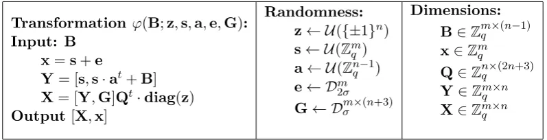
Our randomized transformation ϕis shown in Figure 1. The transformation uses, as random-ness, both a uniform secret vector s and abinary secret vector z. Informally, the intuition is that by simultaneously multiplying by s(on the left) and byz (on theright), the same transformation is able to produce (depending on how the inputB was chosen) either
• a binary LWE distribution with secret z (whenB is uniform), or
• a (transposed4) standard LWE distribution with secret [s,St]t(whenB= (AS+E)t).
Intuitively, one may think of ϕ as mapping B to [B,Bz+e]. So, when B is uniformly random, ϕoutputs the binary LWE distribution by construction. On the other hand, if B= (AS+E)t= StAt+Et, the transformation outputs [B,Bz+e] =St[At,Atz] + [Et,Etz+e], which looks like a standard (transposed) LWE label matrix. In fact, by the Leftover Hash Lemma, one may argue
4
Transformation ϕ(B;z,s,a,e,G): Input: B
x=s+e
Y= [s,s·at+B] X= [Y,G]Qt·diag(z) Output [X,x]
Randomness: z← U({±1}n) s← U(Zmq ) a← U(Znq−1) e← Dm
2σ G← Dσm×(n+3)
Dimensions: B∈Zmq ×(n−1) x∈Zmq
Q∈Znq×(2n+3) Y∈Zm×n
q X∈Zm×n
q
Figure 1: Transformation proving the pseudorandomness of binary LWE, where Q is the matrix specified in Lemma 7.
that [At,Atz] is statistically close to a uniformly distributed matrix. Unfortunately, the error matrix [Et,Etz+e] does not follow the Gaussian distribution5 required by LWE. So, in order to address this and other technical difficulties, the actual transformationϕis a bit more complex. The details of the transformation are somewhat technical, and they are primarily motivated by all the cancellations needed for the proof to work and obtain the proper LWE Gaussian error distribution. One way to gain additional insight into the construction is to notice that the transformation ϕ(B) always outputs a pair [X,x] such that Xz=s+Gv≈s+e=x. (See proof of Claim 1 for details.) So, distribution ˆB=ϕ(B) will also satisfy this property with high probability: there must be a small vector ˆz ∈ {±1}n+1 such that (AˆˆS+Eˆ)tˆz ≈ 0. This shows that the pseudorandom
matrix Bˆ = (AˆˆS+Eˆ)t is already somehow close to a binary LWE instance because there is a ±1 combination of the first n columns of Bˆ that is close to the last column. In fact, something very similar can be proved directly, without using ϕ: matrixAˆt maps a set {0,1}n+1 of size 2n > qk+1
to a setZkq+1 of sizeqk+1. So, by the pigeon-hole principle, there exist two binary inputs such that ˆ
Atˆz0 =Aˆtzˆ1, or, equivalently, a small vectorˆz=ˆz0−ˆz1(withkzk∞= 1) such thatBˆˆz=Eˆtˆz≈0. An informal interpretation of this argument (which, in fact, is closely related to the proof that LWE is robust with respect to the secret distribution [11]) is that matrix Aˆt hashes the binary secret ˆz to an almost uniform (smaller dimensional) secret Aˆtˆz with entries in Zq. But, as before, the
problem with this intuitive approach is that the error distribution Eˆtˆz is not Gaussian, and it is correlated with the secretˆz.
Our theorem below solves these technical problems using a carefully designed gadget matrix Q (described in Lemma 7) which efficiently adjusts the error distribution using some extra randomness G. Notice how, in the process of transforming LWE into binary LWE, the number of samplesn−1 in the presumed hardLWE(q, k×m, n−1, σ) instance becomes the sizenof the secret in the final binary LWE instance LWE±(q, n, m,σˆ). Similarly, the number of columnsm (i.e., the number of parallel LWE instances) in the presumed hardLWE(q,(k+ 1)×m, n+ 1,2σ) instance becomes the number of samples in the final binary LWE instance.
Theorem 1 Assume the distributionsLWE(q, k×m, n−1, σ) andLWE(q,(k+ 1)×m, n+ 1,2σ)
are pseudorandom. If q≤2nO(1), σ≥ω(√logn),k≥ω(logn), andn≥(k+ 1)·log2(q) +ω(logn),
5
then the distribution LWE±(q, n, m,σˆ) is also pseudorandom for σˆ = 2σ√n+ 1.
Proof: We use Zas a shorthand for the diagonal matrixdiag(z). We first show that the transfor-mationϕ maps the uniform distribution to the binary LWE distribution.
Claim 1 If B← U(Zmq×(n−1)) is chosen uniformly at random, then ϕ(B) ∈Zmq×n×Zmq is statis-tically close to theLWE±(q, n, m,σˆ) distribution.
Proof: We show that for any fixed values ofa ∈Zn−1
q and z ∈ {±1}n, the output of the
transfor-mation [X,x] =ϕ(B) is statistically close to theLWE±distribution with secret z, i.e.,X∈Zm×n q
is uniformly random, and the conditional distribution of the noise vectorˆe=x−Xz(givenX and z) is statistically close to Dm
ˆ
σ. All this is over the probability space defined by the random choice
of B,s,e,G. The claim follows by averaging over aand z.
LetQ= [Q[n],Q]n[] be the matrix defined in Lemma 7, and recall thatQ[n]∈Zn×nis invertible,
utQ[n] =et1, and the vector vt =utQ]n[∈Zn+3 has normkvk= 2 √
n, kvk∞ ≤2. Since s and B are uniformly random, the matrix Y is also uniformly distributed, and independent of e and G. Since Qt
[n] and Zare invertible, the matrix
X= [Y,G][Q[n],Q]n[]tZ=Y(Qt[n]Z) + (GQt]n[Z)
is also uniformly distributed, independently of G,e. It remains to analyze the conditional dis-tribution of the error vector ˆe = x−Xz. Using Z·z = u and YQt
[n]u = Ye1 = s, we get
Xz = YQt[n]u+GQt]n[u = s+Gv. So, the error vector equals ˆe = (s+e)−Xz = e−Gv. Since the entries of G and e are independent discrete Gaussians of parameter σ and 2σ (respec-tively), the coordinates ofˆeare independent identically distributed random variables, each follow-ing the distribution D2σ−PiviDσ. By Lemma 5, this distribution is statistically close to Dσˆ for
ˆ
σ=p(2σ)2+P
i(viσ)2 =σ
p
4 +kvk2 = 2σ√n+ 1.
Next, consider the output [X,x] whenB follows distribution B.
Claim 2 The distribution ϕ(B) is statistically close to Bˆ.
Proof: Let B= (AS+E)tforA← U(Zq(n−1)×k),S← U(Zkq×m) and E← D
(n−1)×m
σ . By linearity,
we can writeY= [s,sat+B] =Ys+Ye as the sum of two matrices
Ys= [s,sat+StAt] and Ye= [0,Et].
Similarly, we can also decomposeϕ(B) = [X,x] = [Xs,s] + [Xe,e] as a sum where
Xs=YsQt[n]Z and Xe= [Ye,G]QtZ= [Et,G]Qt]1[Z.
Our goal is to show that [Xs,s]t=AˆˆS and [Xe,e]t=Eˆ forA,ˆ S,ˆ Eˆ distributed as in the definition
of ˆB.
We first look at the distribution of the error matrixEˆt= [X
e,e]. The last columneis a discrete
Gaussian of parameter 2σ by construction. Since [Et,G] has Gaussian distributionDσm×(2n+2), the
rest of the matrix is distributed according to
Xet ←ZtQ]1[(Dσ(2n+2)×m)≈Z(Dn ×m
2σ ) =D n×m
for any fixed value ofz, where we have used the property Q]1[(Dσ2n+2)≈ D2nσ from Lemma 7, and
the symmetry ZDn
2σ =Dn2σ. This proves thatEˆ has Gaussian distribution of parameter 2σ, and it
depends only on E,Gand e.
We now look at the distribution of [Xs,s] = (AˆˆS)t over the random choice ofa,s,z,A and S.
The idea is to set Sˆ = [s,St]t, so thatSˆ is distributed uniformly at random overZ(qk+1)×m. But, in
order to properly randomize Aˆ, we define
ˆ
S=W−1
st S
whereW is a uniformly random invertible matrix inZq(k+1)×(k+1). Since W is invertible,Sˆ is still
uniformly distributed, and independent ofW. Next, define
ˆ A=
I zt
ZQ[n]HW∈Zq(n+1)×(k+1) where H=
1 0t a A
∈Znq×(k+1).
Using the identitiesztZQ[n]=utQ[n]=e1t and HWˆS=H[s,St]t =Yst, we see that our choice of ˆ
A,Sˆ satisfies (AˆˆS)t = [Xs,s] as desired. All that is left to do is to prove that Aˆ is statistically
close to uniform, independently of ˆS. We first look atHW. Letwt be the first row ofW. That’s
also the first row ofHW. The remaining rows ofHWare [a,A]W. The first rowwtis distributed uniformly at random among all primitive vectors in Zkq+1, i.e., all vectors such that gcd(w, q) = 1.
So, by Lemma 2, the vectorwis within negligible statistical distance from the uniform distribution over Zkq+1. Finally, since [a,A] is uniform by construction, and W is invertible, the bottom rows
([a,A]W) ofHWare uniform too, and independent ofw. So,HW is statistically close to uniform overZnq×(k+1). The matrixAˇ = (ZQ[n]HW)tis also statistically close to uniform (and independent
of z) because Q[n] and Z are invertible. Finally, using the Leftover Hash Lemma (Lemma 1) and
the assumptionn≥(k+1) log2(q)+ω(logn), we see thatAˆt=Aˇ[I,z] = [A,ˇ Azˇ ] is also statistically close to uniform. This concludes the proof that ϕ(B) = (AˆˆS+Eˆ)t where A,ˆ ˆS and Eˆ follow the LWE distribution as in the definition of ˆB.
We are now ready to prove the theorem. It follows from pseudorandomness of the LWE(q, k×
m, n−1, σ) that the distribution Bis computationally indistinguishable from the uniform distribu-tion U over Zmq×(n−1). Since ϕis efficiently computable, the distributions ϕ(B) and ϕ(U) are also
computationally indistinguishable. By Claim 1,ϕ(U) is statistically close toLWE±(q, n×1, m,σˆ). Similarly, by Claim 2,ϕ(B) is statistically close to ˆB. So, LWE±(q, n×1, m,σˆ) is computationally indistinguishable from ˆB. Finally, from the pseudorandomness of LWE(q,(k+ 1)×m, n+ 1,2σ), we know that the distribution ˆBis computationally indistinguishable from the uniform distribution overZmq×(n+1). It follows by transitivity that the binary LWE distributionLWE±(q, n, m,σˆ) is
com-putationally indistinguishable from the uniform distribution overZmq×(n+1), i.e.,LWE±(q, n, m,σˆ)
is pseudorandom.
Corollary 1 Assume the distribution LWE(q, k, n+ 1, σ) is pseudorandom for some q ≤ 2nO(1), σ ≥ ω(√logn), k ≥ ω(logn), and (n + 1) ≥ (k + 1)·(log2(q) + 1). Then the distribution LWE±(q, n, nO(1),σˆ) is also pseudorandom forσˆ = 2σ√n+ 1.
Proof: Notice that, under the assumptions in the corollary statement,
n≥(k+ 1) log2q+k≥(k+ 1) log2q+ω(logn)
as required by Theorem 1. In order to invoke the theorem, we also need to verify the pseudorandom-ness conditions. Assume LWE(q, k, n+ 1, σ) is pseudorandom. Dropping the last two rows from the samples [A,b] ← LWE(q, k, n+ 1, σ) shows that LWE(q, k, n−1, σ) is also pseudorandom. The samples [A,b] can also be mapped to LWE(q, k+ 1, n+ 1,2σ) by performing the following two operations:
• Add an extra Gaussian error term e ← Dn√+1
3σ to b. By Lemma 5, this has the effect of
increasing the error rate to√σ2+ 3σ2 = 2σ.
• Append an extra columnatoAand add a random multiplea·stob. This has the effect of extending the secret with an extra coordinates.
Since this transformation also preserves the uniform distribution, it provides a reduction from LWE(q, k, n+ 1, σ) to LWE(q, k+ 1, n+ 1,2σ), and proves that LWE(q, k+ 1, n+ 1,2σ) is pseu-dorandom. Finally, by Lemma 8,LWE(q, k×m, n−1, σ) andLWE(q,(k+ 1)×m, n+ 1,2σ) are also pseudorandom, as required by Theorem 1.
Notice how Corollary 1 establishes the pseudorandomness ofLWE±for any polynomial number of samples m = nO(1), using, as an assumption, only the pseudorandomness of LWE for a fixed number (n+ 1 ≈ klogq) of samples. (This property is also implicit in [6].) We remark that we phrased Theorem 1 and Corollary 1 asymptotically (in terms of polynomial-time distinguishers achieving at most negligible advantage =n−ω(1)) only for simplicity. All statements and proofs are easily adapted to other settings, e.g., to prove hardness of binary LWE against adversaries running in subexponential time.
4
Conclusion
We presented a simple proof that the LWE problem with binary secret of sizen=O(klog2q) is as hard as LWE with uniformly random secret inZkq. More specifically, if LWE with secrets inZkq and n≈klogq samples is pseudorandom, then LWE with secrets in{0,1}nor{±1}n(and an arbitrary
An important open problem is whether similar results can be proved for the structured variants of LWE based on algebraic lattices [15, 14]. The use of structured lattices is of primary importance to make lattice cryptography efficient in practice, and the use of LWE with binary secrets plays an important role in some applications, like Fully Homomorphic Encryption schemes [9, 8], to control the noise growth when computing on encrypted data. We remark that the use of binary secrets and errors does not seem to pose any difficulty in the setting of one-way hash functions based on structured lattices [15]. However, for LWE [21, 14], it is unclear how to adapt the proof in this paper to the algebraic lattice setting. We hope our simple proof for unstructured lattices will bring more attention to this problem, and serve as a possible starting point to establish similar results for ring LWE.
Acknowledgments The author thanks the anonymous Theory of Computing referees and editor Oded Regev for useful comments on earlier drafts of this paper.
References
[1] M. R. Albrecht. On dual lattice attacks against small-secret LWE and parameter choices in HElib and SEAL. In Proceedings of EUROCRYPT 2017, volume 10211 of Lecture Notes in Computer Science, pages 103–129, 2017.
[2] M. R. Albrecht, C. Cid, J. Faug`ere, R. Fitzpatrick, and L. Perret. Algebraic algorithms for LWE problems. ACM Comm. Computer Algebra, 49(2):62, 2015.
[3] B. Applebaum, D. Cash, C. Peikert, and A. Sahai. Fast cryptographic primitives and circular-secure encryption based on hard learning problems. InProceedings of CRYPTO 2009, volume 5677 ofLecture Notes in Computer Science, pages 595–618. Springer, 2009.
[4] S. Arora and R. Ge. New algorithms for learning in presence of errors. InAutomata, Languages and Programming - Proceedings of ICALP 2011, Part I, volume 6755 of Lecture Notes in Computer Science, pages 403–415. Springer, 2011.
[5] S. Bai and S. D. Galbraith. Lattice decoding attacks on binary LWE. In Information Security and Privacy - Proceedings of ACISP 2014, volume 8544 ofLecture Notes in Computer Science, pages 322–337. Springer, 2014.
[6] Z. Brakerski, A. Langlois, C. Peikert, O. Regev, and D. Stehl´e. Classical hardness of learning with errors. InSymposium on Theory of Computing - Proceedints of STOC 2013, pages 575– 584. ACM, 2013.
[7] J. A. Buchmann, F. G¨opfert, R. Player, and T. Wunderer. On the hardness of LWE with binary error: Revisiting the hybrid lattice-reduction and meet-in-the-middle attack. In Proceedings of AFRICACRYPT 2016, volume 9646 of Lecture Notes in Computer Science, pages 24–43. Springer, 2016.
[9] L. Ducas and D. Micciancio. FHEW: bootstrapping homomorphic encryption in less than a second. In Proceedings of EUROCRYPT 2015, Part I, volume 9056 of Lecture Notes in Computer Science, pages 617–640. Springer, 2015.
[10] C. Gentry, C. Peikert, and V. Vaikuntanathan. Trapdoors for hard lattices and new crypto-graphic constructions. In Symposium on Theory of Computing - Proceedings of STOC 2008, pages 197–206. ACM, 2008.
[11] S. Goldwasser, Y. T. Kalai, C. Peikert, and V. Vaikuntanathan. Robustness of the learning with errors assumption. In Innovations in (Theoretical) Computer Science - Proceedings of I(T)CS 2010, pages 230–240. Tsinghua University Press, 2010.
[12] J. H˚astad, R. Impagliazzo, L. A. Levin, and M. Luby. A pseudorandom generator from any one-way function. SIAM J. Comput., 28(4):1364–1396, 1999.
[13] P. Kirchner and P. Fouque. An improved BKW algorithm for LWE with applications to cryptography and lattices. InProceedings of CRYPTO 2015, Part I, volume 9215 of Lecture Notes in Computer Science, pages 43–62. Springer, 2015.
[14] V. Lyubashevsky, C. Peikert, and O. Regev. On ideal lattices and learning with errors over rings. J. ACM, 60(6):43:1–43:35, 2013. Prelim. version in Eurocrypt 2010.
[15] D. Micciancio. Generalized compact knapsacks, cyclic lattices, and efficient one-way functions.
Computational Complexity, 16(4):365–411, 2007. Prelim. version in FOCS 2002.
[16] D. Micciancio and P. Mol. Pseudorandom knapsacks and the sample complexity of LWE search-to-decision reductions. InProceedings of CRYPTO 2011, volume 6841 ofLecture Notes in Computer Science, pages 465–484. Springer, 2011.
[17] D. Micciancio and C. Peikert. Hardness of SIS and LWE with small parameters. InProceedings of CRYPTO 2013, Part I, volume 8042 ofLecture Notes in Computer Science, pages 21–39. Springer, 2013.
[18] D. Micciancio and O. Regev. Worst-case to average-case reductions based on Gaussian mea-sures. SIAM J. Comput., 37(1):267–302, 2007. Prelim. version in FOCS 2004.
[19] C. Peikert. Public-key cryptosystems from the worst-case shortest vector problem: extended abstract. InSymposium on Theory of Computing - Proceedings of STOC 2009, pages 333–342, 2009.
[20] C. Peikert, O. Regev, and N. Stephens-Davidowitz. Pseudorandomness of ring-LWE for any ring and modulus. InSymposium on Theory of Computing - Proceedings of STOC 2017, pages 461–473, 2017.
[21] O. Regev. On lattices, learning with errors, random linear codes, and cryptography. J. ACM, 56(6):34:1–34:40, 2009. Prelim. version in STOC 2005.