Linear Equivalence of Block Ciphers with Partial
Non-Linear Layers: Application to LowMC
Itai Dinur1, Daniel Kales2, Angela Promitzer3, Sebastian Ramacher2, and Christian Rechberger2
1 Department of Computer Science, Ben-Gurion University, Israel 2
Graz University of Technology, Austria
3 Independent
Abstract. LowMC is a block cipher family designed in 2015 by Al-brecht et al. It is optimized for practical instantiations of multi-party computation, fully homomorphic encryption, and zero-knowledge proofs. LowMCis used in the Picnicsignature scheme, submitted to NIST’s post-quantum standardization project and is a substantial building block in other novel post-quantum cryptosystems. ManyLowMCinstances use a relatively recent design strategy (initiated by G´erard et al. at CHES 2013) of applying the non-linear layer to only a part of the state in each round, where the shortage of non-linear operations is partially compen-sated by heavy linear algebra. Since the high linear algebra complexity has been a bottleneck in several applications, one of the open questions raised by the designers was to reduce it, without introducing additional non-linear operations (or compromising security).
In this paper, we considerLowMCinstances with block sizen, partial non-linear layers of size s ≤ n and r encryption rounds. We redesign LowMC’s linear components in a way that preserves its specification, yet improvesLowMC’s performance in essentially every aspect. Most of our optimizations are applicable to all SP-networks with partial non-linear layers and shed new light on this relatively new design methodology. Our main result shows that whens < n, eachLowMCinstance belongs to a large class of equivalent instances that differ in their linear layers. We then select arepresentative instance from this class for which encryption (and decryption) can be implemented much more efficiently than for an arbitrary instance. This yields a new encryption algorithm that is equiv-alent to the standard one, but reduces the evaluation time and storage of the linear layers from r·n2 bits to about r·n2−(r−1)(n−s)2.
Additionally, we reduce the size ofLowMC’s round keys and constants and optimize its key schedule and instance generation algorithms. All of these optimizations give substantial improvements for smallsand a rea-sonable choice ofr. Finally, we formalize the notion of linear equivalence of block ciphers and prove the optimality of some of our results. Comprehensive benchmarking of our optimizations in variousLowMC applications (such asPicnic) reveals improvements by factors that typ-ically range between 2x and 40x in runtime and memory consumption.
1
Introduction
LowMC is a block cipher family designed by Albrecht et al. [ARS+15], and is heavily optimized for practical instantiations of multi-party computation (MPC), fully homomorphic encryption (FHE), and zero-knowledge proofs. In such ap-plications, non-linear operations incur a higher penalty in communication and computational complexity compared to linear ones. Due to its design strategy, LowMCis a popular building block in post-quantum designs that are based on MPC and zero-knowledge protocols (cf. [BEF18,CDG+17a,DRS18b,KKW18,DRS18a]). Most notably, it is used in thePicnicsignature algorithm [CDG+17b] which is a candidate in NIST’s post-quantum cryptography standardization project.4
Instances of LowMC are designed to perform well in two particular met-rics that measure the complexity of non-linear operations over GF(2). The first metric is multiplicative complexity (MC), which simply counts the number of multiplications (AND gates in our context) in the circuit. The second metric is the multiplicative (AND) depth of the circuit.
The relevance of each metric depends on the specific application. For example, in the context of MPC protocols, Yao’s garbled circuits [Yao86] with the free-XOR technique [KS08] (and many of their variants) have a constant number of communication rounds. The total amount of communication depends on the MC of the circuit as each AND gate requires communication, whereas XOR operations can be performed locally. In an additional class of MPC protocols (e.g., GMW [GMW87]), the number of communication rounds is linear in the ANDdepth of the evaluated circuit. The performance of these protocols depends on both the MC and ANDdepth of the circuit.
In order to reduce the complexity of non-linear operations for a certain level of security,LowMCcombines very dense linear layers over GF(2)n (wherenis
the block size) with simple non-linear layers containing 3×3 Sboxes of algebraic degree 2. TheLowMCblock cipher family includes a huge number of instances, where for each instance, the linear layer of each round is chosen independently and uniformly at random from all invertible n×nmatrices.
The design strategy ofLowMCattempts to offer flexibility with respect to both the MC and ANDdepth metrics. In particular, some LowMC instances minimize the MC metric by applying only apartial non-linear layer to the state of the cipher at each round, while the linear layers still mix the entire state. In general, this approach requires to increase the total number of rounds in the scheme in order to maintain a certain security level, but this is compensated by the reduction in the size of the non-linear layers and the total AND count is generally reduced. The global parameters ofLowMCthat are most relevant for this paper are (1) the block size ofnbits, (2) the number of roundsr(which is determined according to the desired security level), and (3) a parameterswhich
4
denotes the domain length of each non-linear layer, namely, the number of bits on which it operates (which may be smaller thann).5
WhileLowMC’s design aims to minimize the non-linear complexity of the scheme at the expense of using many linear algebra (XOR) operations, in several practical applications, XORs do not come for free and may become a bottleneck in the implementation. This phenomenon was already noted and demonstrated in the original LowMC paper. Indeed, due to the large computational cost of LowMC’s dense linear layers, one of the open problems raised by its designers was to reduce their computational cost, presumably by designing more specific linear layers that offer the same security level with improved efficiency.
More recently, the high cost of LowMC’s linear operations influenced the design of the Picnic signature algorithm, where the most relevant metric is the MC that affects the signature size. In order to minimize the AND count (and the signature size), the LowMC instances used byPicnic should have a very small partial non-linear layer in each round (perhaps using only a single 3×3 Sbox). However, such an instance has a large number of roundsrand each encryption requires computation of r matrix-vector products that increase the signing and verification times. Consequently, the Picnic designers settled for non-linear layers of intermediate size in order to balance the signature size on one hand and the signing and verification times on the other.
In fact, in Picnic there is another source of inefficiency due to the heavy cost of the linear operations in LowMC’s key schedule: the computation of LowMC inside Picnic involves splitting the LowMC instance to 3 related instances which are evaluated with a fresh share of the key in each invocation. Therefore, in contrast to standard applications, the key schedule has to be run before each cipher invocation and it is not possible to hard-code the round keys into the LowMCinstance in this specific (and very important) application. In LowMC, each of ther+ 1 round keys is generated by applying an independent n×κrandom linear transformation to theκ-bit master key. Therefore, the total complexity of the key schedule is (r+ 1)·n·κin both time and memory, which is a substantial overhead on the signing and verification processes inPicnic.
Our Contribution In this paper we revisit the open problem of theLowMC designers to reduce the complexity of its linear operations, focusing on instances with partial non-linear layers (i.e., s < n). We consider a generalizedLowMC construction in which ther linear layers are selected uniformly at random from the set of all invertible matrices and the non-linear layers are arbitrary and applied tosbits of the n-bit internal state in each of therrounds. Our results are divided into several parts.
1. The round keys and constants of a generalizedLowMCcipher require mem-ory of (r+ 1)·nbits. We compress them ton+r·sbits. We then consider LowMC’s linear key schedule (with a master key of sizeκbits) and reduce 5
its complexity from (r+ 1)·n·κton·κ+r·(s·κ). This has a substantial effect on the performance ofPicnic, as described above.
2. The linear algebra of the encryption (and decryption) algorithm requires matrices of sizer·n2bits and performs matrix-vector products with about the same complexity. We describe a new algorithm that uses matrices requiring onlyr·n2−(r−1)(n−s)2bits of storage and about the same linear algebra time complexity (using standard matrix-vector products6).
3. We consider the complexity of generating a generalized LowMC instance, assuming its linear layers are sampled at random. We devise a new sampling algorithm that reduces this complexity7from aboutr·n3ton3+(r−1)·(s2·n). Our sampling algorithm further reduces the number of uniform (pseudo) random bits required to sample the linear layers from aboutr·n2ton2+(r− 1)·(n2−(n−s)2). These optimizations are useful in applications that require frequent instance generation, e.g. for the RASTA design strategy [DEG+18]. 4. We address the question of whether the linear layer description we use during encryption is optimal (i.e., minimal) or can be further compressed. Indeed, it may seem that the formulan2+ (r−1)(n2−(n−s)2) is suboptimal, and the formulan2+ (r−1)·s·n2is more reasonable, as it is linear ins(similarly to the reduction in the size of the round keys). However, we prove (under two assumptions which we argue are natural) that no further optimizations that reduce the linear layer sizes are possible without changing their functionality. Table 1 summarizes our improvements and the assumptions under which they can be applied to an SP-network with partial non-linear layers. Surprisingly, al-though the open problem of theLowMCdesigners presumably involved chang-ing the specification ofLowMC’s linear layers to reduce its linear algebra com-plexity, our improvements achieve this without any specification change. All of these improvements are significant forsnandrthat is not too small.
We stress that our optimized encryption algorithm is applicable to any SP-network with partial non-linear layers (such as Zorro8 [GGNS13]) since it does not assume any special property of the linear or non-linear layers. Yet, if the linear layers are not selected uniformly at random, the question of whether our algorithm is more efficient compared to the standard one depends on the spe-cific design. On the other hand, when designing new SP-networks with partial non-linear layers, one may use our optimized linear layers as a starting point for additional improvements. We further note that the reduced complexity of the linear layer evaluation during encryption is also useful for adversaries that attempt to breakLowMCinstances via exhaustive search.
6
Optimizations in matrix-vector multiplications (such as the “method of four Rus-sians” [ABH10]) can be applied to both the standard and to our new encryption algorithm.
7
Using asymptotically fast matrix multiplication and invertible matrix sampling al-gorithms will reduce the asymptotic complexity of both the original and our new algorithm. Nevertheless, it is not clear whether they would reduce their concrete complexity for relevant choices of parameters.
8
Metric Unoptimized Optimized Sect. Assumption RK and RC M (r+ 1)·n n+s·r 3.1 None KS T /M (r+ 1)·(n·κ) n·κ+r·(s·κ) 3.2 Linear KS LL evaluation T /M r·n2 n2+ (r−1)·(n2−(n−s)2) 5 None
LL sampling T r·n
3
n3+ (r−1)·(s2·n)
7 Random LL
R r·n2 n2+ (r−1)·(n2−(n−s)2) sampling
Table 1.Improvements in time/memory/randomness (T /M/R) and assumptions un-der which they are applicable (RK = round keys, RC = round constants, KS = key schedule, LL = linear layer).
Parameters Memory Runtime
n s r LowMC Picnic
128 30 20 2.38x 1.41x 1.34x
192 30 30 3.99x 2.48x 1.72x
256 30 38 4.84x 2.82x 2.01x
128 3 182 16.51x 6.57x 4.74x
192 3 284 31.85x 11.50x 7.97x
256 3 363 39.48x 16.18x 10.83x
Table 2.Multiplicative gains (previous / new) in memory consumption and in runtimes forLowMCencryption andPicnicsigning and verification.
Table 2 compares9 the size of
LowMC’s linear layers in previous implemen-tations to our new encryption algorithm for several instances. The first three instances are the ones used by thePicnicsignature algorithm and for them we obtain a multiplicative gain of between 2.38x and 4.84x in memory consumption. Runtime-wise we obtain an improvement of a factor between 1.41x to 2.82x for LowMC encryption and by a factor between 1.34x to 2.01x forPicnic.
Even more importantly, prior to this work, reducings(in order to optimize the MC metric) while increasingr(in order to maintain the same security level for aLowMC instance) increased the linear algebra complexity proportionally to the increase in the number of rounds, making those instances impractical. One of the main consequences of this work is that such a reduction insnow also reduces the linear algebra complexity per round, such that the larger number of rounds is no longer a limiting factor. In particular, the last three instances in Table 2 correspond to a choice of parameters with a minimal value ofsthat minimizes signature sizes in Picnic. For those instances, we reduce the size of the linear layers by a factor between 16.51x to 39.48x and improve runtimes by up to a factor of 16x. Moreover, compared to the original Picnic instances that uses= 30, using our optimizations, instances with s= 3 reduce memory consumption and achieve comparable runtime results.
9
Our Techniques The first step in reducing the size of the round keys and constants is to exchange the order of the key and constant additions with the application of the linear layer in a round of the cipher. While this is a common technique in symmetric cryptography, we observe that in case s < n, after re-ordering, the constant and key additions of consecutive rounds can be merged through then−sbits of the state that do not go through the non-linear trans-formation. Applying this process recursively effectively eliminates all the key and constant additions onn−s bits of the state (except for the initial key and constant additions). We then exploit the linear key schedule of LowMC and compute the reduced round keys more efficiently from the master key.
In order to derive our new encryption algorithm, we show that each (gen-eralized) LowMC instance belongs to a class of equivalent instances which is of a very large size when s n. We then select a representative member of the equivalence class that can be implemented efficiently using linear algebra optimizations which apply matrices with a special structure instead of random matrices (yet the full cipher remains equivalent). This requires a careful exami-nation of the interaction between linear operations in consecutive rounds which is somewhat related to (but more complex than) the way that round keys and constants of consecutive rounds interact. After devising the encryption algo-rithm, we show how to sample a representative member of an equivalence class more efficiently than a random member. Our new sampling algorithm breaks dependencies among different parts of the linear layers in a generalizedLowMC cipher, shedding further light on its internal structure.
Finally, we formalize the notion of linear equivalence among generalized LowMC ciphers. This allows us to prove (based on two natural assumptions) that we correctly identified the linear equivalence classes and hence our descrip-tion of the linear layers is optimal in size and we use the minimal amount of randomness to sample it. The formalization requires some care and the proof of optimality is somewhat standard (indeed, the claim that we prove is non-standard).
Related Work Previous works [BB02,BCBP03] investigated equivalent rep-resentations of AES and other block ciphers obtained by utilizing the spe-cific structure of their Sboxes (exploiting a property called self-affine equiv-alence [BCBP03]). On the other hand, our equivalent representation and en-cryption algorithm is independent of the non-linear layer and can be applied regardless of its specification. Yet we only deal with block ciphers with partial non-linear layers in this paper.
instance generation algorithm for sampling the linear layers is given in Section 7. Finally, we prove the optimality of our description of the linear layers in Section 8 and conclude in Section 9.
2
Preliminaries
2.1 Notation
Given a string of bits x ∈ {0,1}n, denote by x[|d] its d most significant bits
(MSBs) and byx[d|] itsdleast significant bits (LSBs). Given stringsx, y, denote byxkytheir concatenation. Given a matrixA, denote byA[∗, i] itsi’th column, byA[∗, d|] its firstdcolumns and byA[∗,|d] its lastdcolumns. Given two ma-trices A∈GF(2)d1×d2 andB ∈GF(2)d1×d3 denote by AkB ∈GF(2)d1×(d2+d3)
their concatenation. Denote by Id∈GF(2)d×d the identity matrix.
Throughout this paper, additionx+y between bit stringsx, y∈ {0,1}n is
performed bit-wise over GF(2)n (i.e., by XORing them).
2.2 Generalized LowMC Ciphers
We study generalizedLowMC (GLMC) ciphers where the block size isn bits, and each non-linear layer operates on s≤nbits of the state. Each instance is characterized by a number of roundsr, round keyskifori∈ {0, . . . , r}and round
constantsCi, fori∈ {0, . . . , r}. The cipher consists ofr(partial) invertible
non-linear layersSi :{0,1}s→ {0,1}s andr invertible linear layersLi ∈GF(2)n×n
fori∈ {1, . . . , r}.
A GLMC instance is generated by choosing eachLi independently and
uni-formly at random among all invertiblen×nmatrices.10However, we note that the main encryption algorithm we devise in Section 5 is applicable regardless of the way that the linear layers are chosen. We do not restrict the invertible non-linear layers.
The encryption procedure manipulates n-bit words that represent GLMC states, while breaking them down according to their s LSBs (which we call “part 0 of the state”) and n−s MSBs (which we call “part 1 of the state”). To simplify our notation, given any n-bit stringx, we denote x(0) =x[s|] and x(1)=x[|n−s].
The basic GLMC encryption procedure is given in Algorithm 1. Decryption is performed by applying the inverse operations to a ciphertext.
Key Schedule The key schedule optimization of Section 3.2 assumes that round keys are generated linearly from the master key (as in LowMC) and we now define appropriate notation. The master key k is of lengthκbits. It is used to generate round key ki for i ∈ {0,1, . . . , r} using the matrix Ki ∈ GF(2)n×κ,
namely,ki=Ki·k. During instance generation, each matrix{Ki}ri=0 is chosen uniformly at random among alln×κmatrices.
10
Input :x0 Output :xr+1 begin
x1←x0+k0+C0 fori∈ {1,2, . . . , r}do
yi←Si(x
(0)
i )kx
(1)
i
xi+1←Li(yi) +ki+Ci
end
returnxr+1 end
Algorithm 1:Basic encryption.
2.3 Breaking Down the Linear Layers
Given Li (which is an n×nmatrix), we partition its n-bit input into the first
s LSBs (part 0 of the state that is output bySi) and the remainingn−s bits
(part 1 of the state). Similarly, we partition itsn-bit output into the firstsLSBs (that are inputs ofSi+1) and the remainingn−sbits. We define 4 sub-matrices ofLi that map between the 4 possible pairs of state parts:
L00i ∈GF(2)s×s, Li01∈GF(2)s×(n−s),
L10i ∈GF(2)(n−s)×s, Li11∈GF(2)(n−s)×(n−s). Thus, in our notationLab
i fora, b∈ {0,1}maps the part of the state denoted by
b to the part of the state denoted bya.
Li=
L00
i L01i
L10i |{z}
s
L11i |{z}
n−s
}s }n−s
We extend our notationLab
i by allowinga, b∈ {0,1,∗}, where the symbol ‘∗‘
denotes the full state. Therefore,
Li0∗∈GF(2)s×n, Li1∗∈GF(2)(n−s)×n, L∗i0∈GF(2)n×s, Li∗1∈GF(2)n×(n−s),
are linear transformations which are sub-matrices of Li, as shown below.
Li=
L0i∗ L1∗
i
,Li=
L∗0
i L∗i1
These linear transformation satisfy several basic equalities, e.g., for each y ∈ {0,1}n:
L0i∗(y) =Li(y)(0) =L00i (y(0)) +L01i (y(1)),
L1i∗(y) =Li(y)(1) =L10i (y
(0)) +L11
i (y
2.4 Complexity Evaluation
In this paper, we analyze the complexity of the linear layers of generalized LowMC schemes. We will be interested in the two natural measures of time complexity (measured by the number of bit operations) and memory complexity (measured by the number of stored bits) of a single encryption (or decryption) of an arbitrary plaintext (or ciphertext). The linear layers are naturally repre-sented by matrices, and thus evaluating a linear layer on a state is a simply a matrix-vector product. Since the time and memory complexities of evaluating and storing the linear layers are proportional in this paper, we will typically refer to both as the linear algebra complexity of the linear layers. For algorithms that generate GLMC instances, we will be interested in time complexity and in the number of random bits (or pseudo-random bits) that they use.
3
Optimized Round Key Computation and Constant
Addition
In this section we optimize the round key computation and constant addition in a GLMC cipher. First, we show how to compress the round keys and constants and then we optimize the key schedule of the cipher, assuming it is linear. These optimizations are significant in case we need to run the key schedule for every cipher invocation (which is the case inPicnic).
3.1 Compressing the Round Keys and Constants
We combine the last two linear operations in encryption Algorithm 1 and obtain xi+1←Li(yi)+ki+Ci. Moreover,yi ←Si(x
(0)
i )kx
(1)
i , namelySionly operates on
the firstsbits of the state and does not changex(1)i . Based on this observation, we perform the following:
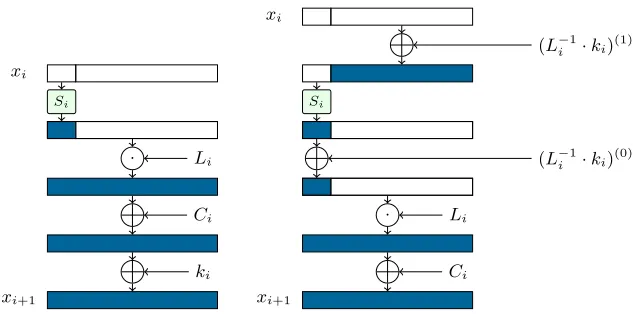
– Modifyxi+1←Li(yi) +ki+Ci toxi+1←Li(yi+Li−1·ki) +Ci.
– SplitL−i1·ki into the lower sbits (the “non-linear part”, i.e., (L−i 1·ki)(0))
and the uppern−sbits (the “linear part”, i.e., (L−i1·ki)(1)) and move the
addition of the uppern−sbits before the Sbox layer.
Figure 1 demonstrates one round of the cipher with the above modifications (which do not change its output).
Next, we observe that the addition of (L−i1·ki)(1) at the beginning of the
xi
Si
· Li
Ci
ki
xi+1
xi
(L−1
i ·ki)(1)
Si
(L−1
i ·ki)(0)
· Li
Ci
xi+1
Fig. 1.One round before (left) and after (right) splitting the round key addition.
In total, the size of the round keys is reduced fromn·(r+ 1) ton+s·r. We remark that the same optimization can be performed to the constant additions, reducing their size by the same amount. We denote the new reduced round key of roundibyk0iand the new reduced round constant byCi0. The new encryption procedure is given in Algorithm 2. Observe that all the values{k0
i+Ci0}ri=0can be computed and stored at the beginning of the encryption and their total size isn+s·r.
Input :x0 Output :xr+1 begin
x1←x0+k00 +C
0
0 fori∈ {1,2, . . . , r}do
yi←(Si(x(0)i ) +k
0
i+C
0
i)kx
(1)
i
xi+1←Li(yi)
end
returnxr+1 end
Algorithm 2: Encryption with reduced round keys and constants.
3.2 Optimizing the Key Schedule
We now deal with optimizing the round key computation of Algorithm 2, as-suming a linear key schedule. The original key schedule appliesr+ 1 round key matricesKito theκ-bit keykin order to compute the round keyski=Ki·k. It
The main observation is that all transformations performed in Section 3.1 in order to calculate the new round keys from the original ones are linear. These linear transformations can be composed with the linear transformations Ki in
order to define linear transformations that compute the new round keys directly from the master keyk. Since the total size of the round keys isn+s·rbits, we can define matrices of total sizen·κ+r·(s·κ) that calculate all round keys from the masterκ-bit key.
More specifically, we define the matrixL−i1which is the inverse of the linear layer matrix Li, with the first s rows of this inverse set to 0. Applying the
iterative procedure defined in Section 3.1 from round r down to round i, we obtain
PN,i= r
X
j=i j
Y
`=i
L−`1 !
·Kj.
Fori≥1, the new round keyk0i(for the non-linear part of the state) is computed by taking thesleast significant bits ofPN,i·k. Using the notation of Section 2.3,
we have
ki0= (PN,i)0∗·k.
Observe that the total size of all{(PN,i)0∗}ri=1 isr·(s·κ) bits. Finally, the new round keyk0
0 is calculated by summing the contributions from the linear parts of the state, using the matrix
PL=K0+
r
X
j=1
j
Y
`=1 L−`1
! ·Kj.
Therefore, we have k00 = PL ·k, where PL is an n×κ matrix. All matrices
{(PN,i)0∗}ri=1, PL can be precomputed after instance generation and we do not
need to store the original round key matricesKi.
4
Linear Algebra Properties
In this section we describe the linear algebra properties that are relevant for the rest of this paper. We begin by describing additional notational conventions.
4.1 General Matrix Notation
The superscript ofLab
i introduce in Section 2.3 has a double interpretation, as
specifying both the dimensions of the matrix and its location inLi. We will use
this notation more generally to denote sub-matrices of somen×nmatrixA, or simply to define a matrix with appropriate dimensions (e.g.,A01∈GF(2)s×(n−s) may be defined without defining Aand this should be clear from the context). Therefore, dimensions of the matrices in the rest of the paper will be explicitly specified in superscript as Aab, where a, b∈ {0,1,∗}(we do not deal with
matrixA, the superscript has a double interpretation as specifying both the di-mensions ofAaband its location inA. When no superscript is given, the relevant
matrix is of dimensions n×n. There will be two exceptions to this rule which will be specified separately.
4.2 Invertible Binary Matrices
Denote by αn the probability that ann×n uniformly chosen binary matrix is
invertible. We will use the following well-known fact:
Fact 1 [[Kol99], page 126, adapted] The probability that an n×n uniform bi-nary matrix is invertible is αn = Q
n
i=1(1−1/2
i) > 0.2887. More generally,
for positive integers d ≤ n, the probability that a d×n binary matrix, cho-sen uniformly at random, has full row rank of d is Qn
i=n−d+1(1−1/2
i) =
Qn
i=1(1−1/2
i)
/ Qn−d
i=1(1−1/2
i)
=αn/αn−d.
We will be interested in invertibility of matrices of a special form, described in the following fact (which follows from basic linear algebra).
Fact 2 Ann×nbinary matrix of the form
A00 A01 A10I
n−s
is invertible if and only if thes×smatrixB00=A00+A01A10 is invertible and its inverse is given by
(B00)−1 −(B00)−1·A01 −A10·(B00)−1I
n−s−A10·(B00)−1·A01
.
Finally, we prove (in Appendix A) a simple proposition regarding random ma-trices.
Proposition 1. LetA∈GF(2)n×n be an invertible matrix chosen uniformly at
random and let B11 ∈ GF(2)(n−s)×(n−s) be an arbitrary invertible matrix (for s≤n) that is independent fromA. Then the matrix
C=
A00A01·B11 A10A11·B11
is a uniform invertible matrix.
4.3 Normalized Matrices
Remark 1. The only exception to the rule of Section 4.1 has to do with Defini-tion 1 (and later with the related DefiniDefini-tion 2). In this paper, the decomposiDefini-tion of Definition 1 is always applied to matrices A1∗ ∈GF(2)(n−s)×n (in caseA1∗ is a sub-matrix ofA, it contains the bottomn−srows ofA). Hence the result-ing matrices ˙A ∈GF(2)(n−s)×(n−s), ¨A ∈GF(2)(n−s)×s and ˆA ∈GF(2)(n−s)×n
have fixed dimensions and do not need any superscript. On the other hand, we will use superscript notation to denote sub-matrices of these. For example
ˆ
A10∈GF(2)(n−s)×sis a sub-matrix of ˆA, consisting of its firstscolumns.
It will be convenient to consider a lexicographic ordering in which the columns indices ofA1∗ are reversed, i.e., the first ordered set ofn−scolumns is{n, n− 1, . . . , s+ 1}, the second is{n, n−1, . . . , s+ 2, s}, etc. To demonstrate the above definition, assume that COL(A) = {n, n−1, . . . , s+ 1} is a consecutive set of linearly independent columns. Then, the matrixA1∗ is shown below.
A1∗= ¨ A |{z} s ˙ A |{z}
n−s
n−s
We can write A= ( ˙A·A˙−1)·A= ˙A·( ˙A−1·A) = ˙A·A, whereˆ ˆ
A= ˙A−1·A1∗= ˙ A−1·A¨ | {z }
s
In−s
| {z }
n−s
n−s. (1)
Normalized Equivalence Classes Given an invertible matrixA∈GF(2)n×n,
define
N(A) = A0∗
ˆ A
=
A0∗ ˙
A−1·A1∗
= I
s 001
010A˙−1
·A.
The transformationN(·) partitions the set of invertiblen×nboolean matrices intonormalized equivalence classes, whereA, Bare in the same normalized equiv-alence class ifN(A) =N(B). We denoteA↔N B the relationN(A) =N(B).
Proposition 2. Two invertiblen×nboolean matricesA, B satisfy A↔N B if
and only if there exists an invertible matrixC11 such that
A=
Is 001
010C11
·B.
For the proof of Proposition 2, we refer the reader to Appendix A.
LetΦ={N(A)|A∈GF(2)n×n is invertible} contain a representative from
each normalized equivalence class. Using Fact 1 and Proposition 2, we deduce the following corollary.
Corollary 1. The following properties hold for normalized equivalence classes:
1. Each member of Φ represents a normalized equivalence class whose size is equal to the number of invertible (n−s)×(n−s) matrices C11, which is αn−s·2(n−s)
2
. 2. The size of Φis
|Φ|= αn·2
n2
αn−s·2(n−s)2
=αn/αn−s·2n
2−(n−s)2
4.4 Matrix-Vector Product
Definition 2. Let A1∗ andB∗1 be two Boolean matrices such that A1∗ has full row rank of n−s. DefineBˇA=B·A˙ ∈GF(2)n×(n−s).
WhenAis understood from the context, we simply write ˇB instead of ˇBA.
Remark 2. The notational conventions that apply to Definition 1 also apply Def-inition 2 (see Remark 1), as it is always applied to matricesA1∗∈GF(2)(n−s)×n
and B∗1 ∈ GF(2)n×(n−s), where ˇB ∈ GF(2)n×(n−s) (and its sub-matrices are denoted using superscript).
Proposition 3. LetA1∗andB∗1be two Boolean matrices such thatA1∗has full row rank ofn−s. LetC=B∗1·A1∗∈GF(2)n×n. Then, after preprocessingA1∗ andB∗1,C can be represented using b=n2−s2+n bits. Moreover, givenx∈ GF(2)n, the matrix-vector productCxcan be computed usingO(b)bit operations.
Note that the above representation of then×nmatrixCis more efficient than the trivial representation that usesn2bits (ignoring the additive lower order term n). It is also more efficient than a representation that uses the decomposition C=B∗1·A1∗ which requires 2n(n−s) = (n2−s2) + (n−s)2≥n2−s2bits. Proof. The optimized representation is obtained by “pushing” linear algebra operations from A1∗ into B∗1, which “consumes” them, as formally described next. Note that sinceA1∗has full row rank ofn−s, we use definitions 1 and 2, and writeC=B∗1·A1∗=B∗1·( ˙A·A˙−1)·A1∗= (B∗1·A)·( ˙˙ A−1·A1∗) = ˇB·A, where ˇˆ B and ˆAcan be computed during preprocessing. Let us assume that the lastn−s columns ofA1∗are linearly independent (namely, COL(A1∗) ={n, n−1, . . . , s+ 1}). Then due to (1), ˆAcan be represented usings(n−s) bits and the matrix-vector productCxcan be computed usingO(s(n−s) +n(n−s)) =O(n2−s2) bit operations by computing ˆAx= ( ˙A−1·A)¨ ·x[s|] +x[|n−s].
We assumed that the last n−s columns of A1∗ are linearly independent. If this is not the case, then COL(A1∗) can be specified explicitly (to indicate the columns of ˆA that form the identity) using at mostn additional bits. The product ˆAxis computed by decomposingxaccording to COL(A1∗) (rather than
according to its sLSBs).
Remark 3. Consider the case that A1∗ is selected uniformly at random among all matrices of full row rank. Then, using simple analysis based on Fact 1,n−s linearly independent columns ofA1∗are very likely to be found among itsn−s+3 last columns. Consequently, the additive low-order termnin the representation size of C can be reduced to an expected size of about 3 logn(specifying the 3 indices among are finaln−s+ 3 that do not belong in COL(A1∗)). Moreover, computing the product ˆAxrequires permuting only 3 pairs of bits ofxon average (and then decomposing it as in the proof above).
Remark 4. Instead of simplifying A1∗ to contain the identity matrix, we can alternatively simplifyB∗1assuming it has full column rank.11It is easy to verify that both simplifications give essentially the same result in terms of linear algebra complexity.
11
Input :x0 Output :xr+1 begin
x1←x0+k0
fori∈ {1,2, . . . , r}do yi←Si(x
(0)
i )kx
(1)
i
xi+1←Li(yi)
end
returnxr+1 end
Algorithm 3:Simplified encryption.
5
Optimized Linear Layer Evaluation
In this section, we describe our encryption algorithm that optimizes the linear algebra of Algorithm 2. We begin by optimizing the implementation of a 2-round GLMC cipher and then consider a generalr-round cipher.
It will be convenient to further simplify Algorithm 2 by definingk000 =k00+C00. For i > 0, we move the addition of ki0+Ci0 into Si by redefining Si00(x
(0)
i ) =
Si(x
(0)
i ) +ki0+Ci0. This makes the Sbox key-dependent, which is not important
for the rest of the paper. Finally, we abuse notation for simplicity and rename k000 andSi00back tok0andSi, respectively. The outcome is given in Algorithm 3.
5.1 Basic 2-Round Encryption Algorithm
We start with a basic algorithm that attempts to combine the linear algebra computation of two rounds. This computation can be written as
x(0)3 x(1)3
! =
L00
2 L012 L102 L112
y2(0) y2(1)
! , x
(0) 2 x(1)2
! =
L00
1 L011 L101 L111
y1(0) y1(1)
! .
Note that x(0)2 and y(0)2 are related non-linearly as y2(0) =S2(x (0)
2 ). On the other hand, since x(1)2 =y(1)2 we can compute the contribution ofy(1)2 to x3 at once from y1 by partially combining the linear operations of the two rounds as
t(0)3 t(1)3
! =
L01
2 L101 L012 L111 L112 L101 L112 L111
y(0)1 y(1)1
!
. (2)
The linear transformation of (2) is obtained from the productL2·L1by ignoring the terms involvingL00
2 andL102 (that operate ony (0)
2 ). Note that (2) defines an n×nmatrix that can be precomputed.
We are left to compute the contribution ofy(0)2 tox3, which is done directly as in Algorithm 3 by
x(0)2 ←L01∗(y1),y (0)
2 ←S2(x (0) 2 ),t
0 3←L
∗0 2 (y
(0)
This calculation involves s×nand n×smatrices. Finally, combining the con-tributions of (2) and (3), we obtain
x3←t3+t03.
Overall, the complexity of linear algebra in the two rounds isn2+ 2sninstead of 2n2 of Algorithm 3. This is an improvement provided that s < n/2, but is inefficient otherwise.
5.2 Optimized 2-Round Encryption Algorithm
The optimized algorithm requires a closer look at the linear transformation of (2). Note that this matrix can be rewritten as the product
t(0)3 t(1)3
! =
L012 L11 2
L101 L111 y (0) 1 y(1)1
!
. (4)
More compactly, this n×n linear transformation is decomposed as L∗21·L11∗, namely, it is a product of matrices with dimensions (n−s)×nandn×(n−s). In order to take advantage of this decomposition, we use Proposition 3 which can be applied sinceL11∗ has full row rank of n−s. This reduces linear algebra complexity of L∗1
2 ·L11∗ from n2 to n(n−s) +n(n−s)−(n−s)2 = n2−s2, ignoring an additive low order term of 3 logn, as computed in Remark 3.
Input :x0 Output:x3 begin
x1←x0+k0 y1←S1(x
(0) 1 )kx
(1) 1 x(0)2 ←L01∗(y1) y(0)2 ←S2(x
(0) 2 ) x3←L∗20(y
(0) 2 ) x3←x3+ ˇL2( ˆL1(y1)) returnx3
end
Algorithm 4: Optimized 2-round encryption.
Input :x0 Output:x3 begin
x1←x0+k0 y1←S1(x
(0) 1 )kx
(1) 1 x(0)2 ←L01∗(y1) z(1)2 ←Lˆ1(y1) y2(0)←S2(x
(0) 2 ) x3←L∗20(y
(0) 2 ) x3←x3+ ˇL2(z
(1) 2 ) returnx3
end
Algorithm 5: Refactored 2-round encryption.
Algorithm 4 exploits the decompositionL∗21·L11∗= ˇL2·Lˆ1. Altogether, the linear algebra complexity of 2 rounds is reduced to
n2+ 2sn−s2= 2n2−(n−s)2
5.3 Towards an Optimized r-Round Encryption Algorithm
The optimization applied in the 2-round algorithm does not seem to generalize to an arbitrary number of rounds in a straightforward manner. In fact, there is more than one way to generalize this algorithm (and obtain improvements over the standard one in some cases) using variants of the basic algorithm of Section 5.1 which directly combines more that two rounds. These variants are sub-optimal since they do not exploit the full potential of Proposition 3.
The optimal algorithm is still not evident since the structure of the rounds of Algorithm 4 does not resemble their structure in Algorithm 3 that we started with. Consequently, we rewrite it in Algorithm 5 such that z2(1) = ˆL1(y1) is computed already in round 1 instead of round 2. The linear algebra in round 2 of Algorithm 5 can now be described using then×ntransformation
x(0)3 x(1)3
! =
L002 Lˇ012 L102 Lˇ112
y2(0) z2(1)
! .
Note thatz(1)2 is a value that is never computed by the original Algorithm 3. When we add additional encryption rounds, we can apply Proposition 3 again and “push” some of the linear algebra of round 2 into round 3, then “push” some of the linear algebra of round 3 into round 4, etc. The full algorithm is described in detail next.
5.4 Optimized r-Round Encryption Algorithm
In this section, we describe our optimized algorithm for evaluating rrounds of a GLMC cipher. We begin by defining the following sequence of matrices.
Fori= 1 : R11∗=L11∗ ˆ
R1= ( ˙R1)−1·R11∗. For 2≤i≤r−1 : Tˇi=L∗i1·R˙i−1
R1i∗=L10i kTˇi11. ˆ
Ri= ( ˙Ri)−1·R1i∗.
Fori=r: Tˇr=Lr∗1·R˙r−1.
Basically, the matrix ˇTi combines the linear algebra of roundi with the linear
algebra that is pushed from the previous round (represented by ˙Ri−1). The matrix ˆRi is the source of optimization, computed by normalizing the updated
round matrix (after computing ˇTi). The byproduct of this normalization is ˙Ri,
which is pushed into roundi+ 1, and so forth.
Before we continue, we need to prove the following claim (the proof is given in Appendix B).
Proposition 4. The matrixR1∗
i has full row rank ofn−sfor alli∈ {1, . . . , r−
Input :x0 Output :xr+1 begin
x1←x0+k0 y1←S1(x(0)1 )kx
(1)
1 .Round 1
x(0)2 ←L0∗
1 (y1) z2(1)←R1ˆ (y1)
fori∈ {2, . . . , r−1}do
yi(0)←Si(x(0)i ) .Roundi
x(0)i+1←L00
i (y
(0)
i ) + ˇT
01
i (z
(1)
i )
zi(1)+1←Rˆi(y(0)i kz
(1)
i )
end yr(0)←Sr(x
(0)
r ) .Roundr
xr+1←L∗r0(y
(0)
r ) + ˇTr(zr(1))
returnxr+1 end
Algorithm 6: Optimizedr-round encryption.
The general optimized encryption algorithm is given in Algorithm 6. At a high level, the first round can be viewed as mapping the “real state” (y(0)1 , y1(1)) into the “shadow state” (x(0)2 , z(1)2 ) using the linear transformation
x(0)2 z(1)2
! = L00 1 L 01 1 ˆ R10
1 Rˆ111
y1(0) y1(1)
! .
In rounds i ∈ {2, . . . , r−1}, the shadow state (y(0)i , zi(1)) (obtained after applying Si(x
(0)
i )) is mapped to the next shadow state (x
(0)
i+1, z (1)
i+1) using the linear transformation
x(0)i+1 zi(1)+1
! =
L00i Tˇi01 ˆ R10i Rˆ11i
y(0)i zi(1)
! .
Finally, in roundr, the shadow state (yr(0), z
(1)
r ) is mapped to the final real
state (x(0)r+1, x(1)r+1) using the linear transformation
x(0)r+1 x(1)r+1
! =
L00
r Tˇr01
L10r Tˇr11
y(0)
r
zr(1)
! .
Complexity Evaluation As noted above, Algorithm 6 appliesrlinear transforma-tion, each of dimensionn×n. Hence, ignoring the linear algebra optimizations for each ˆRi, the linear algebra complexity of each round isn2, leading to a total
(as ˆRi contains the (n−s)×(n−s) identity matrix). Therefore, the total linear
algebra complexity is
r·n2−(r−1)(n−s)2.
Taking Remark 3 into account, we need to add another factor of 3(r−1) logn.
Remark 5. Note that Algorithm 6 is obtained from Algorithm 3 independently of how the instances of the cipher are generated. Hence, Algorithm 6 is applicable in principle to all SP-networks with partial non-linear layers.
Correctness We now prove correctness of Algorithm 6 by showing that its output value is identical to a standard implementation of the scheme in Algorithm 3. For each i∈ {0,1, . . . , r+ 1}, denote by ¯xi the state value at the beginning of
round iin a standard implementation and by ¯yi the state after the application
ofSi. The proof of Proposition 5 are given in Appendix B.
Proposition 5. For each i∈ {1, . . . , r−1} in Algorithm 6, yi(0) = ¯yi(0), x(0)i+1= ¯
x(0)i+1 andzi(1)+1= ( ˙Ri)−1(¯x
(1)
i+1).
Proposition 6. Algorithm 6 is correct, namelyxr+1= ¯xr+1.
Proof.By Algorithm 6 and using Proposition 5, xr+1=L∗r0(y
(0)
r ) + ˇTr(z(1)r ) =L
∗0
r (¯y
(0)
r ) +L
∗1
r ·R˙r−1 ( ˙Rr−1)−1(¯x(1)r )
= L∗r0(¯y(0)r ) +L∗r1(¯y(1)r ) =Lr(¯yr) = ¯xr+1.
6
Applications to LowMC in Picnic and Garbled Circuits
To verify the expected performance and memory improvements, we evaluate both suggested optimizations in three scenarios:LowMCencryption, the digital signature schemePicnic, and in the context of Yao’s garbled circuits. We discuss the details on the choice of LowMC instances and how LowMC is used in Picnicand garbled circuits and their applications in Appendix C. Throughout this section, we benchmarkLowMCinstances with block sizen, non-linear layer sizesandrrounds and simply refer to them asLowMC-n-s-r. For the evaluation in the context ofPicnic, we integrated our optimizations in the SIMD-optimized implementation available on GitHub.12 For the evaluation in a garbled circuit framework, we implement it from scratch. All benchmarks presented in this section were performed on an Intel Core i7-4790 running Ubuntu 18.04.
12
6.1 LowMC
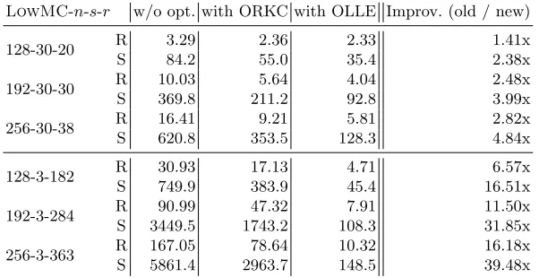
We first present benchmarking results for encryption of LowMC instances se-lected for thePicnic use-case, i.e., with data complexity 1, ands= 3, as well as the instances currently used in Picnic with s = 30. While the optimized round key computation and constant addition (ORKC, Section 3) already re-duces the runtime of a single encryption by half, which we would also obtain by pre-computing the round keys (when not used insidePicnic), the optimized linear layer evaluation (OLLE, Section 5) significantly reduces the runtime even using a SIMD optimized implementation. For s= 30, we achieve improvements by a factor up to 2.82x and fors= 3 up to a factor of 16.18x, bringing the per-formance of the instances with only one Sbox close to ones with more Sboxes.
Memory-wise we observe huge memory reductions for the instances used in Picnic. While ORKC reduces the required storage for the LowMC matrices and constants to about a half, OLLE further reduces memory requirements sub-stantially. As expected, the instances with a small number of Sboxes benefit most significantly from both optimizations. For example, for LowMC-256-10-38 the matrices and constants shrink from 620.8 KB to 128.3 KB, a reduction by 79 %, whereas for LowMC-256-1-363 instead of 5861.4 KB encryption requires only 148.5 KB, i.e., only 2.5 % of the original size. The full benchmark results and sizes of the involved matrices and constants are given in Table 3.
6.2 Picnic
We continue with evaluating our optimizations in Picnic itself. In Table 4 we present the numbers obtained from benchmarking Picnic with the origi-nal LowMC instances, as well as those with s = 3.13 For instances with 10 Sboxes we achieve an improvement of up to a factor of 2.01x. For the extreme case using only 1 Sbox, even better improvements of up to a factor of 10.83x are possible. With OLLE those instances are close to the performance numbers of the instances with 10 Sboxes, reducing the overhead from a factor 8.4x to a factor 1.6x. Thus those instances become practically useful alternatives to obtain the smallest possible signatures.
6.3 Garbled Circuits
Finally, we evaluatedLowMCin the context of garbled circuits, where we pare an implementation using the standard linear layer and round-key com-putation (utilizing the method of four Russians to speed up the matrix-vector products) to an implementation using our optimizations. In Table 5 we present the results of our evaluation. We focus onLowMCinstances with 1 Sbox, since 13
LowMC-n-s-r w/o opt. with ORKC with OLLE Improv. (old / new)
128-30-20 R 3.29 2.36 2.33 1.41x
S 84.2 55.0 35.4 2.38x
192-30-30 R 10.03 5.64 4.04 2.48x
S 369.8 211.2 92.8 3.99x
256-30-38 R 16.41 9.21 5.81 2.82x
S 620.8 353.5 128.3 4.84x
128-3-182 R 30.93 17.13 4.71 6.57x
S 749.9 383.9 45.4 16.51x
192-3-284 R 90.99 47.32 7.91 11.50x
S 3449.5 1743.2 108.3 31.85x
256-3-363 R 167.05 78.64 10.32 16.18x
S 5861.4 2963.7 148.5 39.48x
Table 3.Benchmarks (R) ofLowMC-n-s-rinstances using SIMD, without optimiza-tion, with ORKC, and OLLE (in µs). Sizes (S) of matrices and constants stored in compiled implementation (in KB).
w/o opt. with ORKC with OLLE Improv. (old / new) Parameters Sign Verify Sign Verify Sign Verify Sign Verify
Picnic-128-30-20 3.56 2.41 2.71 1.89 2.65 1.87 1.34x 1.29x Picnic-192-30-30 10.91 7.76 7.52 5.22 6.33 4.44 1.72x 1.75x Picnic-256-30-38 22.80 15.63 15.41 10.82 11.37 7.88 2.01x 1.98x
Picnic-128-3-182 20.49 14.23 11.78 8.28 4.32 3.11 4.74x 4.57x Picnic-192-3-284 80.76 58.23 42.85 29.94 10.13 7.29 7.97x 7.99x Picnic-256-3-363 192.65 139.62 91.77 64.45 18.47 12.89 10.43x 10.83x
Table 4.Benchmarks ofPicnic-n-s-rusing SIMD without optimizations, with ORKC, and OLLE (in ms).
in the context of garbled circuits, the number of AND gates directly relates to the communication overhead. Instances with only 1 Sbox thus minimize the size of communicated data. In terms of encryption time, we observe major improve-ments of up to a factor of 24.72x when compared to an implementation without any optimizations, and a factor of 15.9x when compared to an implementation using the method of four Russians. Since in this type of implementation we have to operate on a bit level instead of a word or 256-bit register as in Picnic, the large reduction of XORs has a greater effect in this scenario, especially since up to 99% of the runtime of the unoptimized GC protocol is spent evaluating the LowMC encryption circuit.
7
Optimized Sampling of Linear Layers
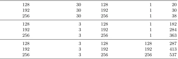
invert-Parameters w/o opt. with M4RM with OLLE Improv. (old / new)
LowMC-128-3-287 8.46 8.01 0.69 12.26x
LowMC-192-3-413 25.26 20.59 1.54 16.40x
LowMC-256-3-537 66.50 40.88 2.69 24.72x
Table 5. Benchmarks of LowMC-n-s-r instances with standard linear layer using method of four Russians (M4RM) and OLLE (in seconds for 210circuit evaluations).
ible matrices. Sampling the linear layers required by Algorithm 6 in a straight-forward manner involves selecting rinvertible matrices and applying additional linear algebra operations that transform them to normalized form. This increases the complexity compared to merely sampling these r matrices in complexity O(r·n3) using a simple rejection sampling algorithm (or asymptotically faster using the algorithm of [Ran93]) and encrypting with Algorithm 3.
We show how to reduce the complexity fromO(r·n3) to14 O(n3+ (r−1)(s2·n)).
We also reduce the amount of (pseudo) random bits requires to sample the linear layers from aboutr·n2to aboutr·n2−(r−1) (n−s)2−2(n−s)
. We note that similar (yet simpler) optimizations can be applied to sampling the key schedule matrices of the cipher (in case it is linear and its matrices are selected at random, as considered in Section 3.2).
The linear layer sampling complexity is reduced in three stages. The first stage breaks the dependency between matrices of different rounds. The second stage breaks the dependency in sampling the bottom part of each round matrix (containingn−srows) from its top part. Finally, the substantial improvement in complexity for smallsis obtained in the third stage that optimizes the sampling of the bottom part of the round matrices. Although the first two stages do not significantly reduce the complexity, they are necessary for applying the third stage and are interesting in their own right.
7.1 Breaking Dependencies Among Different Round Matrices
Recall that for i∈ {2, . . . , r}, the linear transformation of round iis generated from the matrix
L00
i Tˇi01
L10
i Tˇi11
(5) where
ˇ
Ti=L∗i1·R˙i−1.
For i = r, this gives the final linear transformation, while for i < r, the final transformation involves applying the decomposition of Definition 1 toL10
i kTˇi11.
Since ˇTidepends on the invertible (n−s)×(n−s) matrix ˙Ri−1(computed in the 14
previous round), a naive linear transformation sampling algorithm would involve computing the linear transformations in their natural order by computing ˙Ri−1 in roundi−1 and using it in roundi. However, this is not required, as the linear transformation of each round can be sampled independently. Indeed, by using Proposition 1 with the invertible matrixB11= ˙R
i−1, we conclude that in roundi we can simply sample the matrix given in (5) as a uniform invertiblen×nmatrix without ever computing ˙Ri−1. Therefore, the linear transformation sampling for roundrsimplifies to selecting a uniform invertiblen×nmatrix,Lr. For rounds
i∈ {1, . . . , r−1}, we can select a uniform invertiblen×nmatrix,Li, and then
normalize it and discard ˙Ri after the process. This simplifies Algorithm 6, and
it can be rewritten as in Algorithm 7. Note that we have renamed the sequence {z(1)i } to{x(1)i }for convenience.
We stress that the dependency between the round matrices could be broken in Algorithm 7 only since the linear transformation in each round is a uniform invertible matrix. If this is not the case, one can still rename the matrices of Algorithm 6 and derive an algorithm of the form of Algorithm 7. However, computing these matrices would still require deriving ˇTi and ˆRi as defined in
Section 5.4.
Input :x0 Output :xr+1 begin
x1←x0+k0
fori∈ {1, . . . , r−1}do yi←Si(x
(0)
i )kx
(1)
i .Roundi
xi+1←L0i∗(yi)kLˆi(yi)
end
yr←Sr(x(0)r )kx(1)r .Roundr
xr+1←Lr(yr)
returnxr+1 end
Algorithm 7: Simplified and optimizedr-round encryption.
7.2 Reduced Sampling Space
We examine the sample space of the linear layers more carefully.
For each of the first r−1 rounds, the sampling procedure for Algorithm 7 involves selecting a uniform invertible matrix and then normalizing it according to Definition 1. However, by Corollary 1, since each normalized equivalence class contains the same number of αn−s·2(n−s)
2
an explicit representation of the matrices and using an arbitrary ordering is not efficient in terms of complexity. In the rest of this section, our goal is to optimize the complexity of sampling from Φ, but first we introduce notation for the full sampling space.
Let the setΛrcontainr-tuples of matrices defined as
Λr=Φr−1× {A∈GF(2)n×n is invertible},
whereΦr−1=Φ×Φ . . .×Φ | {z }
r−1 times .
The following corollary is a direct continuation of Corollary 1. Corollary 2. The following properties hold:
1. Each r-tuple (L1, . . . , Lr−1, Lr) ∈ Λr represents a set of size (αn−s)r−1 ·
2(r−1)(n−s)2 containingr-tuples of matrices (L0
1, . . . , L0r−1, L0r)such that
N(L01), . . . , N(L0r−1), L0r
= (L1, . . . , Lr−1, Lr).
2. Λr contains
|Λr|=
(αn)r·2n 2
(αn−s)r−1·2(r−1)(n−s)2
= (αn)r/(αn−s)r−1·2r·n
2−(r−1)(n−s)2
r-tuples of matrices.
As noted above, sampling fromΛrreduces to sampling the firstr−1 matrices
uniformly fromΦand using a standard sampling algorithm for ther’th matrix.
7.3 Breaking Dependencies Between Round Sub-Matrices
We describe how to further simplify the algorithm for sampling the linear layers by breaking the dependency between sampling the bottom and top sub-matrices in each round. From this point, we will rename the round matrixLi to a general
matrix A ∈ GF(2)n×n for convenience. In order to sample from Φ, the main idea is to sample the bottom n−s linearly independent rows ofA first, apply the decomposition of Definition 1 and then use this decomposition in order to efficiently sample the remainingslinearly independent rows ofA. Therefore, we never directly sample the largern×nmatrix, but obtain the same distribution on output matrices as the original sampling algorithm.
Output :B,ˆ COL(B1∗)
begin B1∗
←0(n−s)×n,B˙ ←0(n−s)×(n−s)
COL(B1∗)← ∅, rank←0
fori∈ {n, n−1, . . . ,1}do B1∗[∗, i]←GenRand(n−s,1)
if rank=n−sor B1∗[∗, i]∈span( ˙B)then
continue end
rank←rank+ 1 COL(B1∗
)←COL(B1∗ )∪ {i} ˙
B[∗, rank]←B1∗[∗, i]
end
if rank=n−sthen
ˆ
B←( ˙B)−1·B1∗
returnB,ˆ COL(B1∗)
else
returnFAIL
end end
Algorithm 8: SampleBottom() itera-tion
Output :Round matrix for Algorithm 7
begin
ˆ
B,COL(B1∗)←
SampleBottom()
A1∗←Bˆ
C00←GenInv(s) A001←GenRand(s, n−s)
D10←( ˆB·P)10
A000←C00+A001·D10 A0∗←(A000kA001)·P−1 returnA
end
Algorithm 9: Optimized round matrix sampling.
The Optimized Round Matrix Sampling Algorithm Let us first as-sume that after application of Algorithm 8, we obtain ˆB,COL(B1∗) such that COL(B1∗) includes then−slast columns (which form the identity matrix in
ˆ
B). The matrixAis built by placing ˆB in its bottomn−scolumns, and in this case it will be of the block form considered in Fact 2. There is a simple formula (stated in Fact 2) that determines if such matrices are invertible, and we can use this formula to efficiently sample the top s rows of A, while making sure that the fulln×nmatrix is invertible. In case COL(B1∗) does not include then−s last columns, then a similar idea still applies since A would be in the special form after applying a column permutation determined by COL(B1∗). Therefore, we assume thatAis of the special form, sample the topsrows accordingly and then apply the inverse column permutation to these rows. Algorithm 9 gives the details of this process. It uses a column permutation matrix, denoted byP (computed from COL(B1∗), such that ˆB·P = ( ˙B)−1·B¨
kIn−sis of the required
form. The algorithm also uses two sub-procedures:
1. GenRand(n1, n2) samples ann1×n2 binary matrix uniformly at random. 2. GenInv(n1) samples a uniform invertiblen1×n1 matrix.
Proposition 7. Algorithm 9 selects a uniform matrix inΦ, namely, the distri-bution of the output A is identical to the distribution generated by sampling a uniform invertiblen×nmatrix and applying the transformation of Definition 1 to its bottom n−s rows.
For the proof of Proposition 7 we refer the reader to Appendix D.
7.4 Optimized Sampling of the Bottom Sub-Matrix
For small values ofs, the complexity of Algorithm 9 is dominated by Algorithm 8 (SampleBottom()), whose complexity isO((n−s)3+s2(n−s)). We now show how to reduce this complexity toO(s(n−s)) on average. Thus, the total expected complexity of Algorithm 9 becomes
O(s2(n−s) +s3) =O(s2·n)
(using naive matrix multiplication and invertible matrix sampling algorithms). Moreover, the randomness required by the algorithm is reduced from about sn+n(n−s) =n2 to about
sn+ (s+ 2)(n−s) =n2−(n−s)2+ 2(n−s).
Below, we give an overview of the algorithm. Its formal description and analysis are given in Appendix E.
Recall that the output ofSampleBottom() consists of ˆB,COL(B1∗), where ˆ
B contains In−s and s additional columns of n−s bits. The main idea is to
directly sample ˆB without ever sampling the full B1∗ and normalizing it. In order to achieve this, we have to artificially determine the column set COL(B1∗) (which contains the identity matrix in ˆB), and the values of the remaining s columns.
Remark 6. In general, the distribution of ˆBin some alternativeSampleBottom() implementation does not have to be identical to the one of Algorithm 8, as we can select COL(B1∗) in a different way (i.e., using a different method to enumerate the columns). The important requirement is that under any enumeration, ˙B·
ˆ
B =B1∗ should be a uniform matrix of full row rank. Consider the following trivial optimization attempt of SampleBottom(): sample COL(B1∗) uniformly at random among all column sets ofn−sindices (and then sample the remaining columns of ˆB uniformly). This algorithm does not satisfy the requirement, as the distribution of ˙B·Bˆ for ˆB sampled with this algorithm gives more weight to any matrix with many sets of n−s linearly independent columns over any matrix with fewer such sets.
1. In SampleBottom(), full rank is not reached (i.e.,rank < n−s) and col-umniis added to COL(B1∗). Equivalently, the currently sampled vector in SampleBottom() is not in the subspace spanned by the previously sampled vectors (whose size is 2rank). This occurs with probability 1−2rank/2n−s=
1−2(n−s)−rank and can be simulated exactly by (at most) (n−s)−rank
coin tosses in the optimized algorithm (without sampling any vector). 2. In SampleBottom(), full rank is not reached (i.e.,rank < n−s) and
col-umn i is not added to COL(B1∗). This is the complementary event to the first, which occurs with probability 2(n−s)−rank. In SampleBottom(),
such a column i is sampled uniformly from the subspace spanned by the previously sampled vectors whose size is 2rank. The final multiplication
with ( ˙B)−1 is a change of basis which transforms the basis of the pre-viously sampled columns to the last rank vectors in the standard basis e(n−s)−rank+1, e(n−s)−rank+2, . . . , en−s. Hence, column i is a uniform
vec-tor in the subspace spanned by e(n−s)−rank+1, e(n−s)−rank+2, . . . , en−s and
the optimized algorithm samples a vector from this space (usingrankcoin tosses).
3. InSampleBottom(), full rank is reached (i.e.,rank=n−s). The optimized algorithm samples a uniform column using n−s coin tosses. This can be viewed as a special case of the previously considered one, forrank=n−s. Note that no linear algebra operations are performed by the optimized algorithm and it consists mainly of sampling operations.
Decryption We conclude this section by considering efficient sampling of lin-ear layers for decryption. The inverse of the round encryption matrix is of the form shown in Fact 2 after a row permutation (which is the inverse of a column permutation induced by COL(B1∗)). This inverse is generated as a byproduct of Algorithm 9 above for sampling the encryption matrix (which uses the optimized sampling algorithm). Furthermore, matrix-vector product with the inverse ma-trix (during decryption) can be computed in aboutn2−(n−s)2bit operations, hence decryption can be performed in about the same complexity as encryption.
8
Optimality of Linear Representation
In this section, we prove that the representation of the linear layers used by Algorithm 7 for a GLMC cipher is essentially optimal. Furthermore, we show that the number of uniform (pseudo) random bits used by the sampling algorithm derived in Section 7 is close to optimal. More specifically, we formulate two assumptions and prove the following theorem under these assumptions, recalling the value of |Λr|from Corollary 2.
Theorem 1. Sampling an instance of a GLMC cipher with uniform linear lay-ers must use at least
b= log|Λr|= log (αn)r/(αn−s)r−1·2r·n
2−(r−1)(n−s)2
≥
uniform random bits and its encryption (or decryption) algorithm requires at leastbbits of storage on average. Moreover, if a secure PRG is used to generate the randomness for sampling, then it must produce at leastbpseudo-random bits and the encryption (and decryption) process requires at leastb bits of storage on average, assuming that it does not have access to the PRG.
We mention that the theorem does not account for the storage required by the non-linear layers. The theorem implies that the code size of Algorithm 7 is optimal up to an additive factor of about r·(3.5 + 3 logn), which is negligible (less than 0.01·bfor reasonable choices of parameters).
8.1 Basic Assumptions
The proof relies on the following two assumptions regarding a GLMC cipher, which are further discussed in Appendix F.
1. If a PRG is used for the sampling process, it is not used during encryption. 2. The linear layers are stored in a manner which is independent of the spec-ification of the non-linear layers. Namely, changing the specspec-ification of the non-linear layers does not affect the way that the linear layers are stored.
8.2 Model Formalization
We now define our model which formalizes the assumptions above and allows to prove the optimality of our representation.
Definition 3. Given a triplet of global parameters(n, s, r), a (simplified) stan-dard representation of a GLMC cipher is a triplet R = (k0,S,L) such that k0∈ {0,1}n,S = (S1, S2, . . . , Sr)is anr-tuple containing the specifications ofr
non-linear invertible layersSi:{0,1}s→ {0,1}s andL= (L1, L2, . . . , Lr)is an
r-tuple of invertible matricesLi ∈GF(2)n×n. Ther-tupleLis called a standard
linear representation.
To simplify notation, given a standard representationR= (k0,S,L), we denote the encryption algorithm defined by Algorithm 3 asER:{0,1}n → {0,1}n. Definition 4. Two standard cipher representations R,R0 are equivalent (de-notedR ≡ R0) if for eachx∈ {0,1}n,E
R(x) =ER0(x).
Definition 5. Two standard linear representationsL,L0are equivalent (denoted L ≡ L0) if for each tuple of non-linear layers S, and key k
0, (k0,S,L) ≡ (k0,S,L0).
The requirement that (k0,S,L)≡(k0,S,L0) forany S, k0 captures the sec-ond assumption of Section 8.1 that a standard representation of the linear layers is independent of the non-linear layers (and the key).
8.3 Proof of Theorem 1
We will prove the following lemma regarding linear equivalence classes, from which Theorem 1 is easily derived.
Lemma 1. For anyL 6=L0∈Λ
r,L 6≡ L0.
The lemma states that eachr-tuple ofΛris a member of a distinct equivalence
class, implying that we have precisely identified the equivalence classes.
Proof (of Theorem 1). Lemma 1 asserts that there are at least|Λr|linear
equiva-lence classes. Corollary 2 asserts that eachr-tuple inΛrrepresents a set of linear
layers of size (αn−s)r−1·2(r−1)(n−s) 2
, hence every r-tuple in Λr has the same
probability weight when sampling therlinear layers uniformly at random. The theorem follows from the well-known information theoretic fact that sampling and representing a uniform string (an r-tuple in Λr) chosen out of a set of 2t
strings requires at leastt bits on average (regardless of any specific sampling or
representation methods).
The proof of Lemma 1 relies on two propositions which are implications of the definition of equivalence of standard linear representations (Definition 5). Proposition 8. Let L ≡ L0 be two equivalent standard linear representations. Given k0,S, let R = (k0,S,L) and R0 = (k0,S,L0). Fix any x∈ {0,1}n and i∈ {0,1, . . . , r+ 1}, and denote byxi (resp.xi0) the valueER(x)(resp.ER0(x)) at the beginning of round i. Thenx(0)i =x0i(0).
Namely, non-linear layer inputs (and outputs) have to match at each round when encrypting the same plaintext with ciphers instantiated with equivalent standard linear representations (and use the same key and non-linear layers). Proposition 9. Let L ≡ L0 be two equivalent standard linear representations. Given k0,S, let R = (k0,S,L) and R0 = (k0,S,L0). Fix any x∈ {0,1}n and i∈ {0,1, . . . , r+ 1}, and denote byxi (resp.xi0) the valueER(x)(resp.ER0(x))
at the beginning of roundi. Moreover, fixx¯6=xsuch that x¯i= ¯x
(0)
i ,x¯
(1)
i , where
¯
x(0)i 6=x(0)i , butx¯(1)i =x(1)i . Then, x¯0i(1)=x0i(1).
The proposition considers two plaintextsxand ¯x whose encryptions under the first cipher in roundidiffer only in the 0 part of the state. We then look at the second cipher (formed using equivalent standard linear representations) and claim that the same property must hold for it as well. Namely, the encryptions of xand ¯xunder the second cipher in roundi differ only on the 0 part of the state. For the proofs of Propositions 8 and 9 and Lemma 1, we refer the reader to Appendix G.