Discrete differential operators for computer graphics

(1)

Thesis by Mark Meyer

Advisor Alan H. Barr

In Partial Fulfillment of the Requirements for the Degree of

Doctor of Science

California Institute of Technology Pasadena, California

(Defended May 2004)

(2)

(3)

Acknowledgements

There are many people without whose guidance and support this work would not have been possible. To them I now offer my thanks. First and foremost, I thank my advisor, Alan Barr, for his sage advice and unwavering enthusiasm and encouragement. He has provided a wonderful insight into the world of serious research and helped to nurture my interest in solving challenging intellectual problems. The combination of his knowledge, creativity, and approachability still amazes me.

I am also deeply indebted to the other faculty members who offered unofficial advisement in both research and life. To Mathieu Desbrun, who showed through both his teaching and personal example that with a strong work ethic and creativity, great problems could be tackled. His intelligence and broad range of knowledge didn’t hurt either – and were always of great help in my research. To Peter Schroeder, who pointed out new directions, challenged existing ideas, and always offered his time and expertise to provide constructive suggestions. I am also very grateful for the help and support of the staff who never complained when my ambition (and disorganization) asked them to go far beyond the call of duty: Louise Foucher, Jeri Chittum, and David Felt.

Special thanks to my officemate Min Chen for always bringing interesting problems and stimulating discussions, as well as an understanding shoulder whenever I needed it. Thanks to all my colleagues who helped me through the years to keep my academic focus as well as my personal sanity. Thank you, Pierre Alliez, Eitan Grinspun, Zo¨e Wood, Matt Hanna, Jessie Stumpfel, Jon Alferness, Steven Schkolne, Tran Gieng, Nathan Litke and Catherine Wong.

Finally, and most importantly, I thank my family and my friends who have become my family. Throughout the years you have offered unconditional love and understanding, many

(4)

times when my actions did not warrant it, all while asking nothing in return. I am a product of your love and support. Saying thank you doesn’t seem like enough

The Research on differential operators was partially supported by the STC for Computer Graphics and Scientific Visualization (ASC-89-20219), IMSC - an NSF Engineering Research Center (EEC-9529152), an NSF CAREER award (CCR-0133983), NSF (DMS-9874082, ACI-9721349, DMS-9872890, and ACI-9982273), the DOE (W-7405-ENG-48/B341492), Intel, Alias|Wavefront, Pixar, Microsoft, and the Packard Foundation.

The work on smoothing was supported by the Academic Strategic Alliances Program of the Accelerated Strategic Computing Initiative (ASCI/ASAP) under subcontract B341492 of DOE contract W-7405-ENG-48. Additional support was provided by NSF (9624957, ACI-9721349, DMS-9874082, DMS-9872890, and ASC-89-20219 (STC for Computer Graphics and Scientific Visualization)), Alias|Wavefront and through a Packard Fellowship.

The research on remeshing was supported in part by IMSC NSF Engineering Research Cen-ter (EEC-9529152), by the ECG project of the EU No IST-2000-26473, and by a NSF CAREER award (CCR-0133983).

(5)

by

Mark Meyer

In Partial Fulfillment of the Requirements for the Degree of

Doctor of Science

Abstract

This thesis presents a family of discrete differential operators. Since these operators are derived taking into account the continuous notions of differential geometry, they possess many similar properties. This family consists of first- and second-order properties, both geometric and para-metric. These operators are then analyzed and their practical use is tested in several example applications.

First, the operators are used in a smoothing application. Due to the properties of the opera-tors, the resulting smoothing algorithm is general, efficient and robust to sampling problems. The smoothing can be applied to many different inputs ranging from images to surfaces to volume data.

Second, a surface remeshing technique using the operators is presented. Given the operators, we present an algorithm that resamples a surface mesh according to several geometric criteria (integrated curvature, directional curvature, geometric distortion). The resulting algorithm is efficient, general and user-tunable.

Next, a surface mesh parameterization technique is presented. Using geometric invariants as-sociated with the discrete operators, we present an efficient, tunable parameterization algorithm that is robust to sampling irregularities in the input model. Using the properties of the differ-ential operators allows us to make a parameterization algorithm that relies only on geometric information and not the original parameterization of the input model.

Finally, we conclude and present future work including physical simulation and sampling theory.

(6)

List of Figures

1.1 Some applications of differential operators: (a) Non-photorealistic renderings [DFRS03] can use curvatures (and their derivatives) to determine where to draw

suggestive contours, (b) a surface smoothing technique using curvature flow to

reduce the noise caused by laser scanning, (c) a remeshing algorithm uses

cur-vature to place more samples in regions of high curcur-vature, where more detail is

present, (d) a parameterization algorithm uses differential quantities to minimize

distortion. . . . 2

2.1 Local regions: (a) an infinitesimal neighborhood on a continuous surface patch; (b) a finite-volume region on a triangulated surface using Voronoi cells, or (c)

Barycentric cells. . . 16

2.2 (a) 1-ring neighbors and angles opposite to an edge; (b) Voronoi region on a non-obtuse triangle; (c) External angles of a Voronoi region. . . 21

2.3 Pseudo-code for regionAMixed on an arbitrary mesh . . . 22

2.4 Curvature plots of a triangulated saddle using pseudo-colors: (a) Mean, (b) Gaussian, (c) Minimum, (d) Maximum. . . 29

2.5 Mean curvature plots revealing surface details for: (a) a Loop surface from an 8-neighbor ring, (b) a horse mesh, (c) a noisy mesh obtained from a 3D scanner

and the same mesh after smoothing. Our operator performs well on irregular

sampling such as on the ear of the horse. Notice also how the operator correctly

computes quickly varying curvatures on the noisy head while returning slowly

varying curvatures on the smoothed version. (d) An example of our principal

directions computed on a triangle mesh. . . 30

(12)

3.1 (a): Original 3D photography mesh (41,000 vertices). (b): Smoothed version with the scale-dependent operator in two integration step withλdt = 5·10−5, the iterative linear solver (PBCG) converges in 10 iterations. (c),(d): Close-ups

of the eye. All the images in this chapter are flat-shaded to enhance the faceting

effect. . . 35

3.2 (a) A vertex xiand its adjacent faces, (b) one term of its curvature normal formula. 36

3.3 Comparison between (a) the explicit and implicit transfer function forλdt = 1, and (b) their resulting transfer function after 10 integrations. . . 40

3.4 (a): Comparison between filters using L, L2_,_L3_{, and}_L4_{. (b): The scaling to} preserve volume creates an amplification of all frequencies; but the resulting

filter (diffusion+scaling) only amplifies low frequencies to compensate for the

shrinking of the diffusion. . . 41

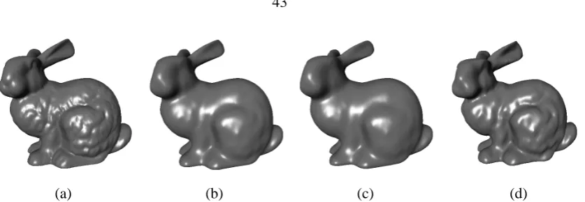
3.5 Stanford bunnies: (a) The original mesh, (b) 10 explicit integrations withλdt= 1, (c) 1 implicit integration withλdt = 10that takes only 7 PBCG iterations (30% faster), and (d) 20 passes of the λ|µ algorithm, with λ = 0.6307 and µ = −0.6732. The implicit integration results in better smoothing than the explicit one for the same, or often less, computing time. If volume preservation is

called for, our technique then requires many fewer iterations to smooth the mesh

than theλ|µalgorithm. . . 43

3.6 Frequency confusion: the umbrella operator is evaluated as the vector joining the center vertex to the barycenter of its neighbors. Thus, cases (a) and (b) will

have the same approximated Laplacian even if they represent different frequencies. 47

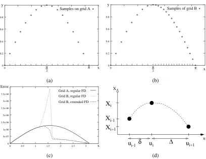
3.7 Test on the heat equation: (a) regular sampling vs. (b) irregular sampling. Nu-merical errors in one step of integration (c): using the usual FD weight on an

irregular grid to approximate second derivatives creates noise, and gives a worse

solution than on the coarse grid, whereas extended FD weights offer the expected

behavior. (d) Three unevenly spaced samples of a function and corresponding

(13)

3.8 Application of operators to a mesh: (a) mesh with different sampling rates, (b) the umbrella operator creates a significant distortion of the shape, but (c) with

the scale-dependent umbrella operator, the same amount of smoothing does not

create distortion or artifacts, almost like (d) when curvature flow is used. The

small features such as the nose are smoothed but stay in place. . . 50

3.9 The area around a vertexxilying in the same plane as its 1-ring neighbors does

not change if the vertex moves within the plane, and can only increase otherwise.

Being a local minimum, it thus proves that the derivative of the area with respect

to the position ofxiis zero for flat regions. . . 52

3.10 Smoothing of spheres: (a) The original mesh containing two different

discretiza-tion rates. (b) Smoothing with the umbrella operator introduces sliding of the

mesh and unnatural deformation, which is largely attenuated when (c) the

scale-dependent version is used, while (d) curvature flow maintains the sphere exactly. . 53

3.11 Significant smoothing of a dragon: (a) original mesh, (b) implicit fairing using

the umbrella operator, (c) using the scale-dependent umbrella operator, and (d)

using curvature flow. . . 54

3.12 Faces: (a) The original decimated Spock mesh has 12,000 vertices. (b) We

lin-early oversampled this initial mesh (every visible triangle on (a) was subdivided

in 16 coplanar smaller ones) and applied the scale-dependent umbrella

opera-tor, observing significant smoothing. One integration step was used,λdt = 10, converging in 12 iterations of the PBCG. Similar results were achieved using the

curvature operator. (c) curvature plot for the mannequin head (obtained using

our curvature operator), (d) curvature plot of the same mesh after a significant

implicit integration of curvature flow (pseudo-colors). . . 55

3.13 From left: Original pretzel shape, smoothing using the Taubin λ/µ algorithm (notice the substantial shape deformation), mean curvature smoothing produces

excellent shape smoothing, and the combined curvature flow plus laplacian

(14)

3.14 From left: Original torus-like shape, smoothing using the Taubinλ/µalgorithm (notice the substantial shape deformation), mean curvature smoothing produces

excellent shape smoothing, and the combined curvature flow plus laplacian

pro-duces a smoothed shape with regularized sampling (image from [OBB00]). . . . 56 3.15 Cube: (a) Original, noisy mesh (±3% uniform noise added along the normal

direction). (b) Isotropic smoothing. (c) Anisotropic smoothing defined in

Sec-tion 3.7.1. . . 57

3.16 Fandisk: (a) Original, noisy mesh. (b) Anisotropic smoothing is performed to

maintain the mesh features while removing the noise. . . 58

3.17 The intensity mapI(x, y)of an image can be thought of as (a) a set of isophotes, or (b) a height field(x, y, z=I(x, y)). . . . 60 3.18 (a): The left side indicates how normals are perpendicular to the screen in

ho-mogeneous, noisy areas, while parallel to the screen plane for edges. The right

side shows how the graph flow is built out of the mean curvature flow by

hav-ing the same magnitude once projected along the normal. (b): W measures the surface expansion between the parameter space (screen pixel) and the surface of

the height field. . . 63

3.19 Examples of denoising for computer-generated greyscale and color images (a

and d: noisy images, b and e: denoised output, c: close-up of a and b). . . 67

3.20 (a) Noisy color image, (b) Denoising flow applied to (a), in 300 explicit iterations

withdt= 1,γ = 0. . . 68

3.21 Clock example: The initial image (a, top) contains a significant amount of noise

as its height field (b) shows. Our denoising technique significantly reduces this

amount of noise (a, bottom) while keeping the features in place (c). . . 68

3.22 Mars elevation map: (a) raw data, (b) smooth version after anisotropic diffusion.

Notice how, with our non-uniform diffusion, the aliasing due to poor

quantiza-tion is suppressed without altering the general topography of the surface (both

pictures are flat-shaded). . . 68

3.23 (a) Head model obtained from a noisy depth image. (b) Reconstructed model

(15)

3.24 Vector field denoising: (a) Original, noisy vector field; (b) Smoothed using

Bel-trami flow; (c) Smoothed using anisotropic weighted flow to automatically

pre-serve the vortex region. . . 69

4.1 A brief overview of our remeshing process: The input surface patch (top left) is first parameterized; Then geometric quantities are computed over the

parame-terization and stored in several 2D maps; These maps are combined to produce

a control map, indicating the desired sampling distribution; The control map is

then sampled using a halftoning technique, and the samples are triangulated,

op-timized and finally output as a new 3D mesh. A few examples of the various types

of meshes our system can produce are shown (top, from left to right): uniform,

increased sampling on higher curvature, the next with a smoother gradation,

regular quads, and semi-regular triangles. After an initial pre-processing stage

(∼1s), each of these meshes was produced in less than 2 seconds on a low-end PC. 73

4.2 Original mesh, conformal parameterization [EDD+95] and texture mapping of a checker-board. Notice the inevitable area distortion on the nose, which we will

automatically compensate for during the resampling process (see Section 4.3.1). . 75

4.3 Examples (in inverse mode for better visualization) of geometry maps for the mask in Figure 4.2. A. M_H, the mean curvature map computed according to [MDSB02]. B. MA, the area map; the nose has been compressed during

the flattening process, while areas nearby the corners have been stretched. C.

Sampling control map, using a per-pixel multiplication:A·B. . . 76

4.4 Area-balanced atlas. From left to right: geometry of a Bunny ear; conformal parameterization and resulting area distortion visualized through a texture

map-ping of a checkerboard; face clustering obtained using [GWH01]; partitioning

obtained by simple bisection [EDD+95, GVSS00]; the conformal parameteriza-tion, with the two medians; area-balanced and smooth partitioning, using the

(16)

4.5 Sampling of the map from Figure 4.3(c) using error diffusion with various num-bers of requested samples (40mseach). . . 82

4.6 Simple example of features: the feature edges (in red) are chained together to create the feature graph; a 1D error diffusion is then performed along the graph

followed by a constrained Delaunay triangulation of the whole sampling; after a

constrained mesh optimization, the feature edges are perfectly preserved, while

blended in the new mesh. . . 85

4.7 Top: Left, Delaunay triangulation over the sampling. Right, after connectivity and geometry optimization. Middle, comparison of valence dispersion. Bottom:

Left, Delaunay triangulation of a sampling performed upon the area map

(lead-ing to uniform mesh) of a mushroom-shape model. Middle, after minimization of

local area dispersion. Right, the remeshed model. Note the uniformity obtained

despite the strong area distortion due to the flattening process. . . 86

4.8 Uniform remeshing of the fandisk. Top: conformal parameterization, and sam-pling obtained by error diffusion with 2.5k vertices with superimposed feature

skeleton. Middle: result of constrained Delaunay triangulation before and after

uniformity optimization. Bottom: several uniform remeshings with 0.2, 0.6, 1.4,

2.5 and 50k vertices respectively. Note the excellent behavior of the 1D error

dif-fusion along the backbones, leading to consistent density between sharp edges

and planar areas. . . 88

4.9 Left: Semi-regular remeshing of a foot model. Right: Mesh created by pasting an image on the importance map (useful for animations and displacement maps). 89 4.10 Uniform remeshing of the MaxPlanck model. In clockwise order: Original mesh;

Conformal parameterization; Parameterization-driven tiling with tree tiles

re-quested; Three tiles meet at a corner; Mesh separation from the tiling; Burst

view of the three tiles after independent uniform remeshing; The tiles put

to-gether require vertex stitching at the boundaries; A post-process swaps some

edges and performs tangential smoothing along the stitching line; and the new

(17)

4.11 Remeshing of the MaxPlanck model with various distribution of the sampling

with respect to the curvature. The original model (left) is remeshed uniformly

and with an increasing importance placed on highly curved areas (left to right)

as the magnified area shows. . . 90

5.1 A piecewise linear mapping between a 3D meshMand an isomorphic flat mesh

U, where a triangle on the mesh is mapped to a triangle in the parameterization. 92 5.2 Intrinsic Parameterizations: Most previous parameterization techniques (b-c)

are not robust to mesh irregularity, exhibiting large distortions for highly

irreg-ular, yet geometrically smooth meshes such as in (a). Non-linear techniques

(d) can achieve much better results, but often require several minutes of

com-putational time. In comparison, with the exact same boundary conditions, our

technique quickly generates very smooth parameterizations, regardless of the

mesh irregularity (sampling quality) as demonstrated by the two texture-mapped

members (e-f) of the novel parameterization family (denoted Intrinsic

Parame-terizations) that we introduce in this chapter. . . 94 5.3 A 3D 1-ring, and its associated flattened version. . . 96

5.4 Other Examples of Natural Conformal Maps: to demonstrate the conformality of the maps we obtain, we use an irregularly sampled mesh and observe that

the symmetry is preserved despite the drastic change in sampling rate. The third

natural parameterization uses the same mesh as in Figure 5.2. These four

pa-rameterizations were obtained in 0.8s, 0.5s, 1.8s, and 0.3s, respectively. . . . . 105 5.5 Left: A 3D surface (top) and its natural conformal parameterization (bottom).

Right: Views of the textured 3D surface. . . 109

5.6 Area Distortion Minimization can be achieved by optimizing the linear com-binationλUA+ (1−λ)Uχ of the conformal and authalic parameterizations. The parameterizations (top) and the area distortion pseudo-coloring (middle)

(18)

5.7 Boundary Optimization: after choosing a (non)linear functional to minimize over the parameterization, we can move the boundary points to perform a

gradi-ent descgradi-ent and optimize the parameterization. Here, an initial irregular

spheri-cal strip is mapped to a circle, then evolves towards an optimized

parameteriza-tion (1.5s) minimizing edge-length distortion. . . 112

A.1 (a) Osculating circle for edge xixj. (b) The integration of the surface gradient

dotted with the normal of the region contour does not depend on the finite volume

discretization used. (c) The area and angle gradients of triangle PAB can be

(19)

Chapter 1

Introduction

1.1

Motivation

The study and estimation of differential quantities on surfaces (such as curvatures) are funda-mental to applications in many fields. Computer Graphics is no exception with many potential applications including (see Figure 1.1):

Rendering / Shading: Shading computations are used in almost every Computer Graphics ap-plication. Programmable shaders allow artists and designers to achieve a wide variety of effects ranging from physically based subsurface scattering to cartoon/cel-shading. These shaders often use a surface’s differential properties for filtering, aiding texture lookups, and general color computations. Non-photorealistic shading techniques [DFRS03], such as diagramatic and toon shading, often use curvatures and their derivatives to determine where to place suggestive contours and where to place shading discontinuities.

Smoothing: Surface smoothing and enhancement algorithms are becoming more and more commonplace in the fields of Computer Graphics, Computer Vision and CAGD (Com-puter Aided Geometrical Design). The use of scanning devices to create surface models has increased rapidly in recent years. While these devices can produce highly detailed models of real-world objects, they also have the inherent problem of noise and scanning errors. Curvature flow as well as other PDEs (partial differential equations) can be used to remove this noise by smoothing the surface.

(20)

(21)

cached on) the parameter domain when it may be difficult to apply the same algorithm to the surface directly – care must be taken, however, to account for the distortion and differences between the surface and the parameter domain. To reduce this problem, these parameterizations are often computed while trying to minimize some notion of distortion (angle differences, length differences, area differences, etc.). These distortion measures often involve differential properties of the surface such as curvatures (and their integrals) and thus can benefit from robust and accurate estimations of these differential properties.

Simulation: With the increased computing power enjoyed today, simulation is becoming a more and more important tool in many fields including Computer Graphics. Simulation allows artists and animators to achieve realistic motions and fine details without requiring the manual specification of every vertex or shaded pixel. This allows the creation of sec-ondary motions and small-scale details that would otherwise have been prohibitively ex-pensive. Simulations also provide predictive power allowing for more efficient tests and experiments that may have been impractical using other means (due to time constraints, expense, safety, etc.). PDEs computed using differential quantities are often used to drive intricate simulations of clothing, skin, muscles, clouds, and fluids just to name a few.

Although differential surface properties have been well studied in other fields, Computer Graphics has one important difference: while most fields use a continuous notion for a surface, in Computer Graphics, we often use a discrete (or at mostC0_{) description of the surface – namely}

triangle meshes. Because of this difference, it is difficult to directly transfer the existing formulae and results to Computer Graphics applications. In fact, despite extensive use of triangle meshes in Computer Graphics and the obviously many uses of differential operators, there is no consen-sus on the most appropriate way to estimate simple geometric attributes such as normal vectors and curvatures on discrete surfaces.

1.2

Contributions

(22)

principal curvaturesκ1 andκ2, and principal directions e1 and e2) for piecewise linear surfaces

such as arbitrary triangle meshes. We present a unified framework for deriving such quantities resulting in a set of operators that is consistent, accurate, robust (in both regular and irregular sampling) and simple to compute. Additionally, as we show, many of these operators can be generalized to any 2-manifold (or even 3-manifold) in an arbitrary dimension embedding space. We then demonstrate the accuracy and usefulness of these operators in several different ge-ometry processing applications:

• An efficient and robust smoothing algorithm that uses the differential operators to inte-grate a surface flow PDE.

• A fast and tunable remeshing algorithm that uses the differential operators in conjunction with user requests to determine where to place the surface samples.

• A parameterization technique that uses the differential properties of the surface to define the distortion metric to be minimized.

1.3

Thesis Overview

The remainder of this dissertation is organized as follows:

Chapter 2 reviews notions and formulae from continuous differential geometry and details why a local spatial average of differential attributes over the immediate 1-ring neighborhood is a good choice to extend the continuous definition to the discrete setting. We then present a formal derivation of the Mean Curvature Normal, Gaussian Curvature, Principal Curva-tures, and Principal Directions for triangle meshes using the mixed Finite-Element/Finite-Volume paradigm. The relevance of our approach is demonstrated by showing the opti-mality of our operators under mild smoothness conditions. Finally, the accuracy of our operators is compared to that of previous techniques.

(23)

Chapter 4 describes a technique for remeshing a triangulated surface. This technique uses the discrete differential operators to drive the placement of samples and the direction of edges. The resulting algorithm is extremely efficient, general and robust.

Chapter 5 describes a technique for parameterizing a triangulated 2-manifold. This technique uses geometric invariants (associated with the properties of our discrete differential opera-tors) to compute sampling invariant, intrinsic parameterizations. These invariants produce efficiently solvable linear systems resulting in an invaluable tool for mesh parameteriza-tion.

(24)

Chapter 2

Discrete Differential Operators

In this chapter, we present a unified and consistent set of flexible tools to approximate important geometric attributes, including normal vectors and curvatures on arbitrary triangle meshes. We present a consistent derivation of these first- and second-order differential properties using

av-eraging Voronoi cells and the mixed Finite-Element/Finite-Volume method, and compare them

to existing formulations. Building upon previous work in discrete geometry, these operators are closely related to the continuous case, guaranteeing an appropriate extension from the continu-ous to the discrete setting: they respect most intrinsic properties of the continucontinu-ous differential operators.

Since differential geometry provides a well researched, formal basis for describing the dif-ferential properties of a surface, we begin with a review of several important quantities from differential geometry (a more complete discussion of differential geometry can be found in one of the many great texts such as [dC76, Gra98, DHKW92]). This is followed by a discussion of previous techniques for computing differential quantities on discrete surfaces. We then present our technique for extending continuous differential operators to the discrete domain using spatial averaging.

2.1

Notions from Differential Geometry

LetS be a surface (2-manifold) embedded in IR3, described by an arbitrary (local) parameteri-zation of 2 variables, X(u, v), around a point p. For each point on the surfaceS, we can locally

(25)

(26)

shape operator or Weingarten mapβ:

β(t) =G−1Dt=−∇_tn,

where t is a vector in the tangent plane at p and−∇tn is the directional derivative of the normal

n in the direction t:

∇_tn= lim

α→0

n(p+αt)−n(p)

α .

Therefore, the shape operator,β, is a linear operator mappingTpS → TpS, whereTpS is the tangent space ofS at p. It measures the change in normal in the direction t and, as we shall see, is useful for measuring the bending and local shape of the surface.

2.1.1 Curvatures and Principal Directions

Local bending of the surface is measured by curvatures. For every unit direction t in the tangent plane, the normal curvatureκN(t) is defined as the curvature of the curve that belongs to both the surface itself and the plane containing both n and t:

κN(t) = β(t)·t

|t|2 .

The two principal curvaturesκ1 andκ2 of the surfaceS, with their associated orthogonal

directions e1and e2, are the extremum values of the normal curvatures over all directions t (see

Figure 2.1(a)). If we parameterize the directions t byθ, the angle between e1 and t, the normal

curvature can be expressed in terms of the principal curvatures:

κN(θ) =κ1cos2(θ) +κ2sin2(θ).

The mean curvatureκH is defined as the average of the normal curvatures:

κH =

1 2π

Z 2π

0

(27)

Using the above relation for normal curvatures, leads to the well-known definition:

κH =

κ1+κ2 2 .

The Gaussian curvatureκGis defined as the product of the two principle curvatures:

κG=κ1κ2. (2.2)

These latter two curvatures represent important local properties of a surface. Points on the surface are often classified based on their mean and Gaussian curvatues – ifκG>0the point is

elliptic, ifκG <0the point is hyperbolic, ifκG = 0andκH 6= 0the point is parabolic, and if

κG=κH = 0the point is planar.

Lagrange noticed thatκH = 0is the Euler-Lagrange equation for surface area minimization.

This gave rise to a considerable body of literature on minimal surfaces and provides a direct relation between surface area minimization and mean curvature flow:

2κH n= lim diam(A)→0

∇A

A ,

whereAis a infinitesimal area around a point p on the surface,diam(A)its diameter, and ∇ is the gradient with respect to the(x, y, z)coordinates of p. We will make extensive use of the mean curvature normalκH n. Therefore, we will denote by K the operator that maps a point

p on the surface to the vector K(p) = 2κH(p) n(p). K is also known as the Laplace-Beltrami

operator for the surfaceS. Note that in the remainder of this chapter we will make no distinction between an operator and the value of this operator at a point as it will be clear from context. Gaussian curvature can also be expressed as a limit:

κG= lim diam(A)→0

AG

A , (2.3)

(28)

2.1.2 Principal Quadric

The portion of a surfaceSnear a point p can be locally represented by the height field (or Monge patch)h(x, y) =z, with p at the origin and the normal n at p in the direction of the z-axis. Using a Taylor Expansion ofhand dropping the higher-order terms results in a quadratic surface which approximatesSto second-order:

z= 1 2(hxxx

2_{+ 2h}

xyxy+hyyy2),

where the derivatives of h are evaluated at p. This surface is known as the principal quadric of Sat p. At an elliptic point, the principal quadric is an elliptic paraboloid; at a hyperbolic point, it is a hyperbolic paraboloid; at a parabolic point, it is a parabolic cylinder; and at a planar point, it is a plane. Note that, since the principal quadric encodes the same differential information as the surfaceS at p, computing the principal quadric is often used as a way to compute the the differential properties ofS.

2.2

Previous Work

Due to the importance of these differential properties in many computer graphics applications, it is no surprise that they have been heavily researched. This section describes several methods for computing differential properties on triangle meshes. In some methods, the vertex normal is computed at the same time as the curvatures. However, some methods require an estimate of the vertex normal to compute the curvature properties. Therefore, we begin by desribing methods for computing the normal at a vertex before discussing techniques for computing the curvatures such as quadric fitting and direct extensions of continuous equations.

In the following sections, assumeT is an oriented triangle mesh with or without boundary. Also assume that the orientation is consistent (neighboring triangles have their normals pointing towards the same side of the surface). For a vertex p, we denote the set of 1-ring neighbors as N1(p)and the number of such neighborsm. Similarly, the 1-ring neighborhood of p is the set

(29)

2.2.1 Vertex Normal Estimation

Since the surface normal is such a fundamental quantity in computer graphics – useful in algo-rithms such as shading, culling, even in computing other differential properties – the computation of vertex normals from a triangle mesh has been studied for many years. It is fairly common to approximate the normal at a vertex p on a triangle mesh by a weighted average of the normals of the triangles incident to p:

n=

P iwini

kP

iwinik

,

where niare the normals of the triangles incident to p.

While the averaging of normals is fairly standard, the choice of the weights wi is not.

Gouraud [Gou71] used an uniformly weighted average, i.e.,wi = 1. Depending on the

arrange-ment of triangles around p, this can produce greatly varying normals. To reduce this problem, Th¨urmer and W¨uthrich [TW98] use the angle incident to p on thei-th face as the weight,wi=θi.

This fits their claim that the normal vector should only be defined very locally, however, this nor-mal remains consistent only if the faces are subdivided linearly, introducing vertices which are not on a smooth surface. Max [Max99] derived weights by assuming that the surface locally approximates a sphere:

wi =

sinθi kpp_ik kpp_i₊₁k,

(30)

2.2.2 Principal Quadric Fitting

One of the most common ways of computing the differential properties at the vertices of a tri-angle mesh is by locally fitting a continuous surface and computing the curvatures on this con-tinuous surface [Ham93]. Since we are intereseted in second-order derivative properties, fitting a quadric intuitively makes sense. In fact, it has been shown that fitting higher-order surfaces has little advantage [KLM98] over fitting quadrics. Therefore, in this section, we will describe techniques for fitting quadrics to triangle meshes and how to recover the associated differential properties1.

While the parameters of the principal quadric could be directly estimated using an procedure to fit to the 1-ring neighbors of p, this results in a non-linear optimization problem. More com-monly, the surface normal is first computed, then the quadric is fit in a rotated space. The steps are as follows:

1. Estimate the surface normal n at p

2. Construct the rotation matrix R= (r1,r2,r3)T:

r1= (I−nn

T₎_i

k(I−nnT₎_i_k, r2 =r3×r1, r3 =n

3. Map the 1-ring data (q_i) into the rotated frame:

˜

qi=R(qi−p)

4. Using the rotated 1-ring neighborsq˜_i, fit the quadric using least squares:

˜

z=a˜x2+b˜x˜y+c˜y2

5. Solve forκ1,κ2, andθ(the angle between thex˜axis and the first principal direction):

κ1,2 =a+c±

p

(a−c)2₊_b2 θ= 1₂atan2(b, a−c)

(31)

Note that this method relies heavily on the accuracy of the normal vector computation. This dependence can be reduced by fitting an extended quadric and iteratively adjusting the normal. The steps remain the same as before except for steps 4 and 5 which become:

4. Fit the extended quadric:

˜

z=a˜x2+b˜x˜y+c˜y2+d˜x+e˜y

This gives a new estimate for the surface normal:

n= (−d,−e,1)

T

(d2₊_e2_{+ 1)}12

From this, a new rotation R can be computed (step 2) and steps 2, 3, 4 can be repeated until the change in normal is below a threshold.

5. Estimate the differential parameters from the extended quadric.

Note that this method could be further extended by adding a translation termf to the extended quadric to account for error in the position of p.

2.2.3 Statistical Methods

When trying to estimate the differential properties of a discrete surface, one of the biggest prob-lems is noise. For this reason, several researchers have looked into statistical methods similar to those in signal processing using covariance matrices. These statistical methods have the benefit of being relatively insensitive to noise. The surface covariance matrix for the 1-ring neighbor-hood of p is:

C₁= 1 m

m X

i=1

(q_i−q)(q¯ _i−q)¯ T,

whereq is the centroid of the neighbors of p. Note that the eigenvectors of this matrix are two¯ tangent vectors t1and t2and the normal n, making the matrixC1similar to the first fundamental

(32)

(33)

matrix:

M= 1

2π

Z π

−π

κN(t)t tTdθ ,

where t is a tangent vector. It can be shown that this3×3symmetric matrix has eigenvalues of 0, λ1, λ2 with the corresponding eigenvectors n,e1,e2. The principal curvatures of the surface

can then be computed as:

κ1= 3λ1−λ2, κ2 = 3λ2−λ1 .

By first estimating the normal, and then projecting each outgoing edge pq_i to define a unit tangent ti, Taubin proposed to approximate the matrixMas:

M= X

qi∈N1(p)

wi κN(ti)titTi ,

where the weightswi are proportional to the areas of the triangles adjacent to the edge pqi,

con-strained so that they sum to unity. The normal curvatureκN(ti)is approximated by constructing

an osculating circle using p, n, and q_iand computing the inverse of its radius:

κN(ti) =

2n·(q_i−p)

kq_i−pk2 .

Once the matrixMis computed, the principal curvatures and directions can easily be recovered using standard eigenvector decomposition techniques.

(34)

Hyman, and Steinberg [HS97, HSS97]. Although it shares a lot of similarities with all these approaches, our work offers a different, unified derivation that ensures accuracy and tight error bounds, leading to simple formulæ that are straightforward to implement.

n

1

e

1

κ

e

2

κ 2

(a) (b) (c)

Figure 2.1: Local regions: (a) an infinitesimal neighborhood on a continuous surface patch; (b)

a finite-volume region on a triangulated surface using Voronoi cells, or (c) Barycentric cells.

2.3

Discrete Properties As Spatial Averages

Most of the smooth definitions for differential properties described above need to be reformulated forC0 _{surfaces. We can consider a mesh as either the limit of a family of smooth surfaces, or}

as a linear (yet assumedly “good”) approximation of an arbitrary surface. Since we wish for the total (integrated) value of the property to be independent of the number of samples in the triangle mesh, we define properties (geometric quantities) of the surface at each vertex as spatial averages around this vertex. This area-averaging is known as the finite volume method. Although this thesis uses piecewise constant weighting functions (in the finite-element/finite-volume sense), more complex weighting functions can easily be incorporated into the area-averaging scheme.

(35)

neighborhood. For example, we define the discrete Gaussian curvature,bκG, at a vertexP as:

b

κG=

1

A Z Z

A

κG dA,

whereAis a properly selected area aroundP. Note however that we will not distinguish between the (continuous) pointwise and the (discrete) spatially averaged notation, except when there may be ambiguity.

2.3.1 General Procedure Overview

The next sections describe how we derive accurate numerical estimates of the first- and second-order operators at any vertex on an arbitrary mesh. We first restrict the averaging area to a family of special local surface patches denotedAM. These regions will be contained within the 1-ring

neighborhood of each vertex, with piecewise linear boundaries crossing the mesh edges at their midpoints (Figures 2.1(b) and (c)). We show that this choice guarantees correspondences be-tween the continuous and the discrete case. We then find the precise surface patch that optimizes the accuracy of our operators, completing the operator derivation. These steps will be explained in detail for the first operator, the mean curvature normal operator, K, and a more direct deriva-tion will be used for the Gaussian curvature operatorκG, the two principal curvature operators

κ1 andκ2, and the two principal direction operators e1and e2. All these operators take a vertex xiand its 1-ring neighborhood as input, and provide an estimate in the form of a simple formula

that we will frame for clarity.

2.4

Discrete Mean Curvature Normal

We now provide a simple and accurate numerical approximation for both the normal vector, and the mean curvature for surface meshes in 3D.

2.4.1 Derivation of Local Integral Using FE/FV

(36)

(37)

(38)

definition minimizeskx−xiksince they contain the closest points to each sample, thus

minimiz-ing the bound on the errorE due to spatial averaging [DFG99]. Furthermore, if we add an extra assumption on the sampling rate with respect to the curvature such that the Lipschitz constants from patch to patch vary slowly with a ratio, we can actually guarantee that the Voronoi cell borders are less thanO() away from the optimal borders. As this still holds in the limit for a triangle mesh, we use the vertices of the mesh as sample points, and pick the Voronoi cells of the vertices as associated finite-volume regions. This will guarantee optimized numerical estimates and, as we will see, determining these Voronoi cells requires few extra computations.

2.4.3 Voronoi Region Area

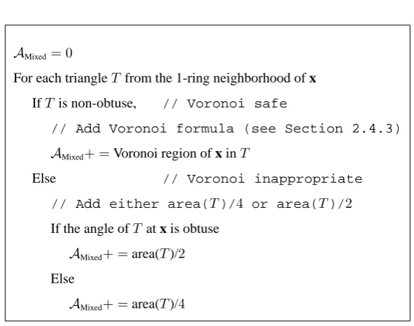
Given a non-obtuse triangleP, Q, Rwith circumcenterO, as depicted in Figure 2.2(b), we must now compute the Voronoi region forP. Using the properties of perpendicular bisectors, we find : a+b+c=π/2, and therefore,a=π/2−_∠Qandc=π/2−_∠R. The Voronoi area for pointP lies within this triangle if the triangle is non-obtuse, and is thus: 1₈(|P R|2_cot_∠_Q+_|_{P Q}_|2_cot_∠_R)_.

Summing these areas for the whole 1-ring neighborhood, we can write the non-obtuse Voronoi area for a vertex xi as a function of the neighbors xj:

AVoronoi=

1 8

X

j∈N1(xi)

(cot αij +cot βij)kxi−xjk2. (2.7)

Since the cotangent terms were already computed for Eq. (2.5), the Voronoi area can be computed very efficiently. However, if there is an obtuse triangle among the 1-ring neighbors or among the triangles edge-adjacent to the ring triangles, the Voronoi region either extends beyond the 1-ring, or is truncated compared to our area computation. In either case our derived formula no longer stands.

2.4.4 Extension To Arbitrary Meshes

(39)

(40)

AMixed = 0

For each triangleT from the 1-ring neighborhood of x IfT is non-obtuse, // Voronoi safe

// Add Voronoi formula (see Section 2.4.3)

AMixed+ =Voronoi region of x inT

Else // Voronoi inappropriate

// Add either area(T)/4 or area(T)/2

If the angle ofT at x is obtuse

AMixed+ =area(T)/2 Else

AMixed+ =area(T)/4

Figure 2.3: Pseudo-code for regionAMixed on an arbitrary mesh

From this expression, we can easily compute the mean curvature value κH by taking half

of the magnitude of this last expression. As for the normal vector, we can just normalize the resulting vector K(xi). In the special (rare) case of zero mean curvature (flat plane or local

saddle point), we simply average the 1-ring face normal vectors to evaluate n appropriately. It is interesting to notice that using the barycentric area as an averaging region results in an operator very similar to the definition of the mean curvature normal by Desbrun et al. [DMSB99], sinceABarycenter is a third of the whole 1-ring areaA1-ring used in their derivation – however, our

new derivation uses non-overlapping regions and is therefore more accurate. At this time, we are not aware of a proof of convergence for this operator. However, our tests have shown no divergence as we refine a mesh, as long as we do not degrade the mesh quality (the triangles must not degenerate). We will give more precise numerical results in Section 2.7.1 showing the improved quality of our new estimate.

2.5

Discrete Gaussian Curvature

In this section, the Gaussian curvatureκGfor bivariate (2D) meshes embedded in 3D is studied.

(41)

(42)

error bounds. In practice, we use the mixed areaAMixedto account for obtuse triangulations. Since

the mixed area cells tile the whole surface without any overlap, we will satisfy the (continuous) Gauss-Bonnet theorem: the integral of the discrete Gaussian curvature over an entire sphere for example will be equal to4π whatever the discretization used since the sphere is a closed object

of genus zero. This result ensures a robust numerical behavior of our discrete operator. Our Gaussian curvature discrete operator can thus be expressed as:

Gaussian Curvature Operator

κG(xi) = (2π−

#f X

j=1

θj)/AMixed (2.9)

Notice that this operator will return zero for any flat surface, as well as any roof-shaped 1-ring neighborhood, guaranteeing a satisfactory behavior for trivial cases. Note also that convergence

conditions (using fatness or straightness) exist for this operator [Fu93, TM02], proving that if the

triangle mesh does not degenerate, the approximation quality gets better as the mesh is refined. We postpone numerical tests until Section 2.7.1.

2.6

Discrete Principal Curvatures

We now wish to robustly determine the two principal curvatures, along with their associated directions. Since the previous derivations give estimates of both Gaussian and mean curvature, the only additional information that must be sought are the principal directions since the principal curvatures are, as we are about to see, easy to determine.

2.6.1 Principal Curvatures

We have seen in Section 2.1 that the mean and Gaussian curvatures are easy to express in terms of the two principal curvaturesκ1 andκ2. Therefore, since bothκH andκGhave been derived

(43)

(44)

(45)

tangent plane:

tij =

(xj−xi)−[(xj −xi)·n]n k(xj−xi)−[(xj −xi)·n]nk

.

A conventional least-square approximation can be obtained by minimizing the errorE:

E(a, b, c) =X

j

wj tTij βtij−κNij 2

.

Adding the two constraintsa+b = 2κH andac−b2 = κG, to ensure coherent results, turns

the minimization problem into a root-finding problem. Once the three coefficients of the matrix B are found, we find the two principal axes e1 and e2 as the two (orthogonal) eigenvectors

ofβ. In practice, all our experiments have demonstrated that the non-linear constraint on the determinant is not necessary (reducing the problem to a linear system). An example of these principal directions is shown in Figure 2.5(b).

Although we could actually determine the principal curvatures (and thus the mean and gaussian curvatures) using an unconstrained least squares procedure (similar to Taubin’s work [Tau95a]), we use our operators to compute the curvatures and only use the least squares for the principal directions as the curvature values computed from the least squares are often less accurate in practice while the directions are fairly robust. A plausible interpretation for the bad numerical properties of a pure least squares approach is the hypothesis of elliptic curvature vari-ation: although this is perfectly valid for smooth surfaces, this is somewhat arbitrary for coarse, triangulated surfaces. It seems therefore more natural to use our previous operators that rely on differential properties still valid on discrete meshes.

2.7

Operator Quality

(46)

2.7.1 Numerical Quality of Our Operators

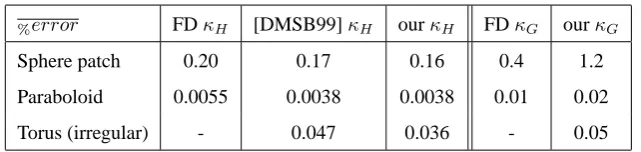
We performed a number of tests to demonstrate the accuracy of our approach in practice. First, we compared our operators to the well-known second-order accurate Finite Difference opera-tors on several discrete meshes approximating simple surfaces such as spheres, or hyperboloids, where the curvatures are known analytically. In order to do so, we used special surfaces defined as height fields over a flat, regular grid so that the FD operators can be computed and tested against our results. The table below lists some representative results:

%error FDκH [DMSB99]κH ourκH FDκG ourκG

Sphere patch 0.20 0.17 0.16 0.4 1.2

Paraboloid 0.0055 0.0038 0.0038 0.01 0.02

Torus (irregular) - 0.047 0.036 - 0.05

Table 2.1: Comparison of our operators with Finite Differences. The error is measured in mean

percent error compared to the exact, known curvature values. Dashes “-” indicate that the

FD tests cannot be performed since the triangulation is irregular. The anglesθj needed for the

Gaussian curvature were computed using the C functionatan2, instead ofacosorasinsince

acosandasinwould significantly deteriorate the precision of the results.

Overall, the numerical quality of our operators is equivalent to FD operators for regular sampling. A major advantage of our new operators over FD operators is that these differential-geometry based operators can still be used on irregular sampling, with the same order of accu-racy.

We also tested our operators against one of the most widely used curvature estimation tech-niques [Tau95a]. We tested several simple surfaces (spheres, parametric surfaces, etc.) to de-termine the effect of sampling on the operators. The surfaces were created with 258 points, quadrisected and reprojected to create surfaces of 1026, 4098 and 16386 points. In all cases, the average percent error of our operators did not exceed 0.07% for mean curvature and 1.3% for gaussian curvature. The previous method had average errors of up to 1.8% for mean curvature and exceeding 10% in some instances for gaussian curvature.

(47)

(a) (b) (c) (d) Figure 2.4: Curvature plots of a triangulated saddle using pseudo-colors: (a) Mean, (b)

Gaus-sian, (c) Minimum, (d) Maximum.

the same order of accuracy as in the fairly regular regions (less than 0.2% average error for mean curvature and below 1.8% average error for gaussian curvature in regions of mild irregularity). The accuracy of our operators decreases as the irregularity (angle and edge length dispersion) increases, but, in practice, the rate at which the error increases is low.

2.7.2 Visual Inspection of Meshes

(48)

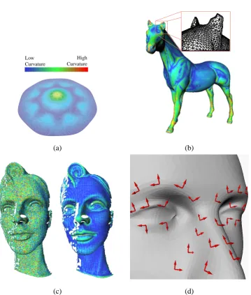
Low Curvature

High Curvature

(a) (b)

(c) (d)

Figure 2.5: Mean curvature plots revealing surface details for: (a) a Loop surface from an

8-neighbor ring, (b) a horse mesh, (c) a noisy mesh obtained from a 3D scanner and the same

mesh after smoothing. Our operator performs well on irregular sampling such as on the ear of

the horse. Notice also how the operator correctly computes quickly varying curvatures on the

noisy head while returning slowly varying curvatures on the smoothed version. (d) An example

of our principal directions computed on a triangle mesh.

2.8

Discrete Operators in

n

D

(49)

(50)

dimen-Gaussian Curvature Operator

The expression of the Gaussian curvature operator Eq. (2.9) still holds innD. Indeed, the Gaus-sian curvature is an intrinsic attribute of a 2-manifold, and does not depend on the embedding.

2.8.2 Beltrami Operator for 3-Manifolds innD

We also extend the previous mean curvature normal operator, valid on triangulated surfaces, to tetrahedralized volumes which are 3-parameter volumes in an embedding space of arbitrary dimension. This can be used, for example, on any MRI volume data (intensity, vector field or even tensor fields). For these 3-manifolds, we can compute the gradient of the 1-ring volume this time to extend the Beltrami operator. Once again, the cotangent formula turns out to be still valid, but this time for the dihedral angles of the tetrahedrons. Appendix A.4 details the derivation to prove this result. This Beltrami operator can still be used to denoise volume data as it minimizes volume just as we denoised meshes through a surface area minimization.

2.9

Conclusion

(51)

Chapter 3

Smoothing

Many times, a triangulated surface does not have the smoothness (or fairness) required for a given application. This problem has increased recently due to the use of highly detailed com-puter graphics objects obtained from imperfectly-measured data from the real-world. When this occurs, the mesh must be smoothed to remove undesirable noise and uneven edges while retain-ing desirable geometric features (see Figure 3.1). In this chapter, we use our discrete differential operators to develop methods to rapidly remove rough features from irregularly triangulated data intended to portray a smooth surface.

Our approach contains several novel features, including an implicit integration method to achieve efficiency, stability, and large time-steps; a scale-dependent Laplacian operator to im-prove the diffusion process; and finally, use of a robust curvature flow operator that achieves a smoothing of the shape itself, distinct from any parameterization. Additional features of the algorithm include automatic exact volume preservation, and hard and soft constraints on the positions of the points in the mesh. Extensions to the smoothing algorithm are also described that allow for feature preservation using anistropic smoothing and simulataneous sampling and shape smoothing using a mixture of Laplacian and curvature flow. The use of higher dimensional smoothing for images, vector fields and volumes is also explored.

We compare our method to previous operators and related algorithms, and prove that our discrete differential operators have several mathematically desirable qualities that improve the appearance of the resulting surface. Finally, we provide a series of examples to graphically and

(52)

numerically demonstrate the quality of our results.

3.1

Introduction

While the mainstream approach in mesh fairing has been to enhance the smoothness of triangu-lated surfaces by minimizing computationally expensive functionals, Taubin [Tau95b] proposed in 1995 a signal processing approach to the problem of fairing arbitrary topology surface tri-angulations. This method is linear in the number of vertices in both time and memory space; large arbitrary connectivity meshes can be handled quite easily and transformed into visually ap-pealing models. Such meshes appear more and more frequently due to the success of 3D range sensing approaches for creating complex geometry [CL96].

Taubin based his approach on defining a suitable generalization of frequency to the case of arbitrary connectivity meshes. Using a discrete approximation to the Laplacian, its eigenvectors become the “frequencies” of a given mesh. Repeated application of the resulting linear operator to the mesh was then employed to tailor the frequency content of a given mesh.

Closely related is the approach of Kobbelt [Kob97], who considered similar discrete ap-proximations of the Laplacian in the construction of fair interpolatory subdivision schemes. In later work this was extended to the arbitrary connectivity setting for purposes of multiresolution editing [KCVS98].

The success of these techniques is largely based on their simple implementation and the increasing need for algorithms which can process the ever larger meshes produced by range sensing techniques. However, a number of issues in their application remain open problems in need of a more thorough examination.

The simplicity of the underlying algorithms is based on very basic, uniform approximations of the Laplacian. For irregular connectivity meshes this leads to a variety of artifacts such as geometric distortion during smoothing, numerical instability, problems of slow convergence for large meshes, and insufficient control over global behavior. The latter includes shrinkage prob-lems and more precise shaping of the frequency response of the algorithms.

(53)

irreg-(a) (b)

(c) (d)

Figure 3.1: (a): Original 3D photography mesh (41,000 vertices). (b): Smoothed version with

the scale-dependent operator in two integration step withλdt = 5·10−5, the iterative linear solver (PBCG) converges in 10 iterations. (c),(d): Close-ups of the eye. All the images in this

chapter are flat-shaded to enhance the faceting effect.

(54)

(55)

In the surface fairing literature, most techniques use constrained energy minimization. For this purpose, different fairness functionals have been used. The most frequent functional is the total curvature of a surfaceS:

E(S) =

Z

S

κ2₁+κ2₂dS. (3.1)

This energy can be estimated on discrete meshes [WW94, Kob97] by fitting local polynomial interpolants at vertices. However, principal curvatures κ1 and κ2 depend non-linearly on the

surface S. Therefore, many practical fairing methods prefer the membrane functional or the thin-plate functional of a mesh X:

Emembrane(X) =

1 2

Z

Ω

X2_u+X2_v dudv (3.2)

Ethin plate(X) =

1 2

Z

Ω

X2_uu+ 2X2_uv+X2_vvdudv. (3.3)

Note that the thin-plate energy turns out to be equal to the total curvature only when the pa-rameterization(u, v) is isometric. Their respective variational derivatives corresponds to the Laplacian and the second Laplacian:

L(X) =Xuu+Xvv (3.4)

L2(X) =L ◦ L(X) =Xuuuu+ 2Xuuvv+Xvvvv. (3.5)

For smooth surface reconstruction in vision, a weighted average of these derivatives has been used to fair surfaces [Ter88]. For meshes, Taubin [Tau95b] used signal processing analysis to show that a combination of these two derivatives of the form: (λ+µ)L −λµL2 _{can provide a}

(56)

3.2.2 Diffusion Equation for Mesh Fairing

As stated above, one common way to attenuate noise in a mesh is through a diffusion process:

∂X

∂t =λL(X). (3.6)

By integrating Equation 3.6 over time, a small disturbance will disperse rapidly in its neighbor-hood, smoothing the high frequencies, while the main shape will be only slightly degraded. The Laplacian operator can be linearly approximated at each vertex by the umbrella operator (we will use this approximation in the current section for the sake of simplicity, but will discuss its validity in section 3.4), as used in [Tau95b, KCVS98]:

L(xi) =

1 m

X

j∈N1(xi)

xj−xi, (3.7)

where xjare the neighbors of the vertexxi, andm= #N1(xi)is the number of these neighbors

(valence). A sequence of meshes(Xn)can be constructed by integrating the diffusion equation with a simple explicit Euler scheme, yielding:

Xn+1 = (I+λdtL)Xn. (3.8)

With the umbrella operator, the stability criterion requiresλdt < 1. If the time step does not satisfy this criterion, ripples appear on the surface, and often end up creating oscillations of growing magnitude over the whole surface. On the other hand, if this criterion is met, we get smoother and smoother versions of the initial mesh asngrows.

3.2.3 Time-Shifted Evaluation

(57)

Implicit integration offers a way to avoid this time step limitation. The idea is simple: if we approximate the derivative using the new mesh (instead of using the old mesh as done in explicit methods), we will get to the equilibrium state of the PDE faster. As a result of this time-shifted evaluation, stability is obtained unconditionally [PFTV94]. The integration is now: Xn+1 =Xn+λdtL(Xn+1). Performing an implicit integration, this time called backward Euler

method, thus means solving the following linear system:

(I−λdtL)Xn+1=Xn. (3.9)

This apparently minor change allows the user not to worry about practical limitations on the time step. Consequent smoothing will then be obtained safely by increasing the valueλdt. However, we now must solve a linear system.

3.2.4 Solving the Sparse Linear System

Fortunately, this linear system can be solved efficiently as the matrix A = I−λdtLis sparse: each line contains approximately seven non-zero elements if the Laplacian is expressed using Eq. (3.7) since the average number of neighbors on a typical triangulated mesh is six. We can use a preconditioned bi-conjugate gradient (PBCG) to iteratively solve this system with great efficiency1. The PBCG is based on matrix-vector multiplies [PFTV94], which only require linear time computation in our case thanks to the sparsity of the matrix A. We review in Appendix A.5 the different options we chose for the PBCG in order to have an efficient implementation for our purposes.

3.2.5 Interpretation of the Implicit Integration

Although this implicit integration for diffusion is sound as is, there are useful connections with other prior work. We review the analogies with signal processing approaches and physical sim-ulation.

1

(58)

(59)

(60)

We also tried to use a linear combination of bothLandL2_{. We obtained interesting results}

like, for instance, amplification of low or middle frequencies to exaggerate large features (refer to [GSS99] for a complete study of feature enhancement). It is not appropriate in the context of a fixed mesh, though: amplifying frequencies requires refinement of the mesh to offer a good discretization.

3.2.7 Constraints

We can put hard and soft constraints on the mesh vertex positions during the diffusion. For the user, it means that a vertex or a set of vertices can be fixed so that the smoothing happens only on the rest of the mesh. This can be very useful to retain certain details in the mesh.

A vertex xi will stay fixed if we impose L(xi) = 0 (or more correctly λ = 0). More

complicated constraints are also possible [BW98]. For example, vertices can be constrained along an axis or on a plane by modifying the PBCG to keep these constraints enforced during the linear solver iterations.

We can also easily implement soft constraints: each vertex can be weighted according to the desired smoothing that we want. For instance, the user may want to smooth a part of a mesh less than another one, in order to keep desirable features while getting a smoother version. We allow the assignment of a smoothing value between0and1to attenuate the smoothing spatially: this is equivalent to choosing a variableλfactor on the mesh, and happens to be very useful in practice. Entire regions can be “spray painted” interactive