Rotation and Turbulent Instability
in Peripheral Heavy Ion Collisions
L.P. Csernai1,aand D.J. Wang1,2,b
1Department of Physics and Technology, University of Bergen, Allegaten 55, 5007 Bergen, Norway 2Key Laboratory of Quark and Lepton Physics (MOE) and Institute of Particle Physics, Central China Normal
University, Wuhan 430079, China.
Abstract.In recent years fluid dynamical processes became a dominant direction of re-search in high energy heavy ion reactions. The Quark-gluon Plasma formed in these reactions has low viscosity, which leads to significant fluctuations and special instabili-ties or flow patterns. One has to study and separate these two effects, but this is not done yet in a systematic way. This presentation presents the most interesting collective flow instabilities, their possible ways of detection and separation form random fluctuations arising from the randomness of the initial configuration in the transverse plane.
1 Introduction
Recent advances in the study of the collective flow properties, have a wide spread of directions. Due to the low viscosity of Quark-Gluon plasma near to the phase transition threshold [1, 2], both significant fluctuations may develop and new Global Collective instabilities may occur, as turbulence in peripheral reactions. The precise analysis of these effects would require the experimental separation of these effects as well as the theoretical study of these effects separately, and then their possible interaction and interference in the observables. The necessity of this separation was pointed out recently [3], and we will elaborate this subject in more detail here.
Another, recent problem is the formation and study of realistic 3+1D initial states in fully realistic description, without unrealistic simplifying assumptions. Here, Fluctuations and Global Collective flow should also be separated, and the Global Collective initial state model should reflect all symme-tries of a heavy ion reaction. This is still not always the case.
In numerous fluid dynamical models, which use the x, y, η, τ coordinates, it is easy to assume uniform longitudinal Bjorken scaling flow, so thatvη = 0, and it is done frequently even in 3+1D
models, this eliminates immediately the longitudinal shear flow, and the arising vorticity. When the longitudinal momentum distribution is uniform in the transverse plane or if it is symmetric around the collision’sz-axis the initial angular momentum is lost, which disables the description of many fundamental phenomena, and also violates the conservation of angular momentum. For a realistic model the longitudinal ends of the initial state (in terms ofz,t orη, τ), they should not exceed the projectile and target rapidities, rather the recoil and the deceleration caused by the other colliding
ae-mail: [email protected]
be-mail: [email protected] C
nucleus should be also taken into account. Only a few models satisfy fully, all conservation laws, and we will discuss the construction of realistic initial state configurations for the Global Collective flow component.
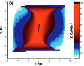
Figure 1.The initial state energy density distribution shown in the Reaction Plane, in the [x,z], plane. This initial state is constructed based on a Glauber model, via fire-streaks, which extend longitudinally. This extension is slowed down by the attractive, chromo-electric, coherent Yang-Mils fields. The resulting string-rope tension is smaller when we have less color charges at the end of the streaks, and this results in a longer streaks and smaller energy density at the top (projectile) and bottom (target) sides. The central streaks that stopped stronger, start a 1D Riemann scaling expansion. This initial state conserves energy, momentum, angular momentum, and shows initial vorticity and longitudinal shear. From ref. [4, 5].
There are few realizations where the conservation laws are fully satisfied. The models generating the initial state from a realistic molecular dynamics or cascade model may reach states close to equi-librium, and the smooth average of such states can serve as an realistic 3+1D initial state. One can also construct a good analytic initial state by taking into account of all symmetries and all conserved quantities and their conservation laws. Such an initial state is described in [4, 5] and presented in Fig. 1.
2 Splitting of Global Collective Flow and Fluctuations
The high multiplicities at high energy heavy ion collisions have enabled us to study fluctuations and the distribution of the azimuthal harmonic components. Due to traditional reasons the azimuthal distributions are parametrized in therms of cosine functions and a separate event-by-event fitted Event Plane azimuth, which did not correlate with the Reaction Plane and had nontrivial correlation among the Event Planes of the different harmonic components.
The non-fluctuating Global Collective (background)1 flow, if the event-by-event center of mass and Reaction plane are identified, (which can be done experimentally, see e.g. ref. [6]) can be written in the form
d3N dydptdφ =
1 2π
d2N dydpt
1+2v1(y−yCM,pt) cos(φ−ΨRP)+ 2v2(y−yCM,pt) cos(2(φ−ΨRP))+· · ·
ΨRP and yCMcan be determined experimentally event-by event, as described in ref. [6]. Notice that the event-by event c.m. fluctuates strongly in the beam direction as due to the large rapidity difference between the projectile and target leading toyCM 0, but also in the transverse plane leading to modifiedΨRP. This second effect was taken into account in ref. [7], without referring to [6], but the stronger longitudinal fluctuations were not studied, and were considered just as "dipole like initial fluctuations".
In contrast to the above formulation fluctuating flow patterns are analysed by using the ansatz
d3N dydptdφ =
1 2π
d2N dydpt
1+2v1(y,pt) cos(φ−ΨEP1 )+ 2v2(y,pt) cos(2(φ−ΨEP2 ))+· · ·
,
which is adequate for exactly central collisions where the Global Collective flow does not lead to azimuthal asymmetries. HereΨEPn maximizesvn(y,pt) in a rapidity range, and bothφandΨEPn are measured in the laboratory (collider) frame.
If this formulation is used for peripheral collisions the analysis is rather problematic, because Global Collective flow patterns and fluctuations are getting mixed up. This is actually also true in central, spherical or cylindrical events but there the separation is more subtle, and it does not show up directly in the azimuthal flow harmonics. Still in special model calculations fluctuations in the transverse plane were studied, and Global Collective flow (background flow) was separated from fluctuations [8].
He we show that the ansatz of flow analysis can be reformulated in a way which makes the split-ting or separation of the Global Collective flow from Fluctuations easier, based on the symmetry requirements arising from the symmetries of the peripheral heavy ion collisions. This formulation is also an ortho-normal series expansion for bothφ-even andφ-odd functions. Considering the relation cos(α−β)=cosαcosβ+sinαsinβ, we can write each of the terms of the harmonic expansion into the form
vncos[n(φ−ΨEPn )]=vncos(nΨEPn ) cos(nφ)+vnsin(nΨEPn ) sin(nφ)
If we consider that the reaction plane,ΨRPcan be determined event-by-event experimentally also [6], we can introduceΦnEP ≡ΨEPn −ΨRP andφ ≡φ−ΨRP, so that from these data we getΨnEP = ΦEP
n + ΨRP. Hereφis the azimuth angle with respect to the Reaction Plane. Now we can also define the new flow harmonic coefficients bycv
n ≡vncos(n(ΦEPn + ΨRP)) andsvn ≡ vnsin(n(ΦEPn + ΨRP)), and we get for the terms of the harmonic expansion
vncos[n(φ−Ψn)]= vncos[n(φ−Φn)] = cvncos(nφ)+ svnsin(nφ). (1)
Thus we have reformulated the azimuthal angle harmonic expansion, which was given originally in terms of cosines and Event Plane angles for each harmonic component, to both sines and cosines in the Reaction Plane as reference plane and the corresponding new coefficientscv
n =cvn(y−yCM,pt) andsv
n=svn(y−yCM,pt). These can be obtained from the measured data,vn,ΨEPn andΨRPdirectly. This form has the advantage that in peripheral collisions the Global Collective (not fluctuating) flow component,cvnfor odd harmonics have to be odd functions of (y−yCM), while for even harmonic components have to be even function of (y−yCM). As the Global Collective flow has to be±y sym-metric in the transverse plane, all the coefficients of the sin(nφ) terms should vanishcv
n =0. These symmetry properties provide a possibility to separate the fluctuating and the global flow (background flow) components.2
When the new coefficientscv
n =cvn(y−yCM,pt) and svn =svn(y−yCM,pt), are constructed, we can conclude thatsvn can be due to fluctuations only. Furthermore for the Global Collective flow, cv
n(y−yCM,pt) must be an even (odd) function of (y−yCM) for even (odd) harmonic coefficients. Due to the fluctuations this is usually not satisfied and one has to construct the even (odd) combinations from the measured data. These represent then the Global Collective component, while the odd (even) combination will represent the Fluctuating component. This separation provides an upper limit for the magnitude of the Global Flow component, because the fluctuations may in some events show the same symmetries as the Global Collective flow. On the other hand for the Fluctuating component, sv
n, provides an upper limit as this component cannot be caused by the Global Collective flow. A last
2In ref.[8] for the longitudinal motion uniformly the Bjorken scaling flow approximation was assumed, which is inadequate
to describe the odd (y−yCM) components. Thus this analysis is limited in the possibility of separating the two components. This is already included in their ansatz of the assumed distribution function,δfiin eq. (2.9) where longitudinal fluctuations
essential guidance may be given by the conditions that the fluctuations must have the same magnitude for sine and cosine components as well as for odd and even rapidity components.
Evaluation of the experimental results this way may provide a better insight into both types of flow patterns. Furthermore, these can also help judgements on theoretical model results, and the theoretical assumptions regarding the initial states.
Other experimental methods, like two particle correlations [9] or polarization measurements [10], may take advantage of this splitting of flow pattern components also.
3 The Initial State
As we have shown the Initial State can be constructed in a way such that all conservations laws are satisfied, and no simplifying assumptions are used, which would violate the conservation laws. In addition there are other principles like causality which should also be satisfied by the initial state.
A frequent simplification inx, y, η, τcoordinates, is to assume uniform longitudinal Bjorken scal-ing flow (this leads to a simple separable initial state distribution function), and in order to satisfy the angular momentum conservation at different transverse points the energy density or mass distribution is made such that on the projectile side a substantial part of the mass is at rapidities exceeding the tar-get and projectile rapidity [11–13]. In most cases this leads to acausal distributions where part of the matter is situated beyond the target and projectile rapidities. This acausality is corrected by Karpenko et al. [14] by cutting the distributions at the target and projectile rapidities. Still the attractive chromo field is not taken into account in this approach, which would limit the initial limiting rapidities by up to 2.5 units of smaller rapidities on each side [15, 16].
Furthermore, the Bjorken scaling flow approach eliminates any possibility for initial shear flow and vorticity, which is a dominant source of simple flow patterns and of strong and visible insta-bilities in classical physics, like rotation and turbulent Kelvin Helmholtz Instability. Apart of the semi-analytic initial state model mentioned in the introduction other initial state models exists, which satisfy all conditions of a realistic initial state. First of all initial state molecular dynamics and multi-particle cascade models which satisfy all conservation laws, boundary conditions and causality, will provide realistic Global Collective initial state as the average of many such realistic events. Also, ana-lytic models can be constructed based on these principles, which are different from the one mentioned in the introduction.
The initial uniform Bjorken scaling flow, is maintained during the fluid dynamical development, so that the lack of shearflow persists in these solutions. It follows that no viscous dissipation takes place in the longitudinal direction, which makes the model configurations anisotropic and not very reliable in this model configurations.3
4 New Global Collective Flow Patterns
As mentioned in the introduction, in collisions of finite impact parameter at high energies we have a large angular momentum which can be as high as J=106 at LHC. The angular momentum is conserved, but due to the explosive expansion of the system the angular velocity of the participant system is rapidly decreasing, thus the local rotation, the vorticity, decreases with time. It depends on
3From the numerical point of view this initial state and this reference frame lead to additional dynamical problems: The
the balance between the expansion and the angular momentum if the rotation will manifest itself in observable quantities at the Freeze out.
FO?
Figure 2.The rotation during the fluid dynamical evolution is indicated by the red arrows pointing to the initial central and corner points on the surface. The motion of these points shows the rotation of the system. The fluid dynamical initial state is preceded by an pre-equilibrium Yang-Mills longitudinal field theoretical model, which took 6.25 fm/c. Thus after 2.00 fm/c fluid dynamical evolution the length of the matter is 8.25 fm (l.h.s). The configuration on the r.h.s. is at 8 fm/c fluid dynamical evolution, which is 14.25 fm/c after the initial touch of the two nuclei. This is just after the estimated freeze out time of 10-12 fm/c. Based on ref. [17].
Due to the widespread use of the uniform longitudinal Bjorken scaling flow in the initial condition, the rotation did not occur in fluid dynamical model calculations, and it was studied only recently. First it was noticed in ref. [17], see Fig. 2.
This rotation acts against the 3rd flow component or antiflow, and may decrease the measured directed flow, or even reveres the direction from antiflow to directed flow. According the calculations [17] thev1 was expected to peak at positive rapidities, but this prediction is strongly dependent on the competition between the rotation and the expansion. The small amplitude ofv1 is difficult to identify in the strongly fluctuating background, without identifying the event-by-event center of mass and Reaction Plane.
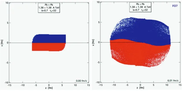
The fluid dynamical calculations with the same method showed for the first time the possibility of the turbulent Kelvin Helmholtz Instability [18]. See Fig. 3. Stability estimates confirmed the possibility of the occurrence if this instability, which could also be obtained in a simple analytic model [19].
5 Detecting the New Flow Patterns via Polarization
The rotation and the turbulence have a small effect on the directed flow, which is weak at RHIC and LHC energies anyway, so alternative ways of detection should be considered.
The angular momentum in case of distributed shear flow, shows up in local vorticity. The simplest classical expression of vorticity in the reaction plane, [x-z], is defined as:
ωy ≡ ωxz ≡ −ωzx≡ 1
FO?
Figure 3. The fluid dynamical development of the shape of the dividing surface between the initial top and bottom halves of the dense matter. The developing non-linear, turbulent wave is the initial stage of a Kelvin Helmholtz Instability. The fluid dynamical initial state indicated by 0.00 fm/c is preceded by an pre-equilibrium Yang-Mills longitudinal field theoretical model, which took 6.25 fm/c indicated by the length of the dense matter. The configuration on the r.h.s. is at 6 fm/c fluid dynamical evolution, which is 12.25 fm/c after the initial touch of the two nuclei. This is just around the estimated freeze out time of 10-12 fm/c. Based on ref. [18]
where the x, y, z components of the 3-velocity u are denoted by vx, vy, vz respectively. In 3-dimensional space the vorticity can be defined as
ω≡ 1
2rotu= 1
2∇ ×u (3)
For the relativistic case, the vorticity tensor,ωμνis defined as
ωμν≡ 1
2(∇νu
μ− ∇μ
uν), (4)
where for any four vectorqμ the quantity∇αqμ ≡ Δβα∂βqμ = Δβαqμ,β and Δμν ≡ gμν −uμuν. The
relativistic generalization of vorticity leads to an increase of the magnitude of vorticity [20].
The local vorticity is decreasing with the expansion, but it is still significant at Freeze out in peripheral collisions due to the huge initial angular momentum. the local vorticity reaches 3 c/fm in the reaction plane [20], which is more than an order of magnitude larger than the vorticity in the transverse plane arising from random fluctuations [21].
This vorticity may lead to two other measurable consequences. According to the equipartition principle for different degrees of freedom carrying the same amount of energy the same applies for angular momentum. Here the local orbital rotation and the spin of the particles may equilibrate with each other. If equilibrium is reached by freeze out the final polarization should have the same direction and magnitude as the local vorticity. Interestingly, high temperature acts against polarization so the polarization is governed by the so called thermal vorticity, where instead of the four velocity,uμ, the inverse temperature four-vector,
βμ(
x)= u
μ(x)
T(x) ,
For the polarization studies it is of utmost importance to identify the proper global directions in a collision event-by event. See Fig. 4. Without identifying the center of mass rapidity, the Reaction
Figure 4.The [x,z], Reaction Plane where the direction of the Projectile and Target matter is indicated. The arising angular momentum,J, points into the−ydirection. When the event-by-event center of mass and the reaction plane is identified this angular momentum is divided between orbital rotation and polarization and spin. The polarization is transverse to the motion of theΛand ¯Λ particles and has the same direction as the angular momentum,J. Thus, this polarization may be detected inΛand ¯Λparticles, which are emitted into the±xdirections. From [10].
Plane, and the Projectile and target side of the reaction plane the detection of the angular momentum and polarization is not possible and earlier measurement at RHIC, where all azimuth angles were averaged over, gave results where the measured polarization was consistent with zero.
TheΛparticle is well suited for measuring its polarization because its dominant decay mode is Λ−→ pπ−and the proton is emitted in the direction of polarization. Notice that due to the thermal and fluid mechanical equilibration process the polarization ofΛs and ¯Λs are the same. This distinguishes the process from electro-magnetic polarization mechanisms.
The thermal vorticity projected to the Reaction Plane is shown in Fig. 5. The thermal vorticity is more pronounced than the standard vorticity, at the external edges of the matter. where the temperature is lower. The thermal vorticity is somewhat larger at RHIC, where the amount of data and the available detector acceptance are larger.
L.P.Csernai 53
RHIC LHC
4.75fm/c 3.56fm/c
Figure 5.The thermal vorticity of the matter arising from a fluid dynamical calculation for two different beam energies. The thermal vorticity is inversely proportional with the temperature, which is increasing faster than the local vorticity with increasing beam energy. Thus the thermal vorticity at RHIC is larger. Also the side regions are cooler and this also increases the thermal vorticity, which enhances the polarization in due to equipartition. Based on ref. [10].
The resulting polarization is shown in Fig. 6. Thus for this measurement the determination of the proper directions of the collision axes is vital. The polarization should be measured forΛs emitted into the±xdirections, which will then be polarized in the−ydirection.
LHC RHIC
Figure 6. The polarization of theΛand ¯Λparticles observed in different directions and at different transverse momenta in the transverse, [x, y] plane at the event-by-event c.m. rapidity for RHIC and LHC energies.
Signifi-cant polarization can be measured for particles at larger momenta,pt≥3 GeV/c, in the±pxdirections. Based on
ref. [10].
ion reactions, which have high initial angular momentum. Unfortunately, even some 3+1D fluid dynamical calculations assume oversimplified initial states where initial shear and vorticity vanishes and these are not able to show these effects.
6 Detecting the New Flow Patterns via Two Particle Correlations
The detection described in the previous section 5, was sensitive to the local vorticity. Two particle correlation measurements are sensitive to the integrated emission from the freeze out space-time zone, the so called "homogeneity" region, where the dominant emission is directed toward the detection, i.e. in the (out)-direction.
Recently we proposed the Differential Hanbury Brown and Twiss method to study the rotation of the source via two particle correlations [9, 22]. The method is based on a simple observation, if we have a spherically symmetric or cylindrically symmetric source with an rotation axis, or any source which is left/right symmetric with respect to a given "out-direction", of momentumk, then we can construct from the usual two particle correlation function with momenta p1 = k+q/2 and p2=k−q/2:
C(k,q)= P2(k+q/2,k−q/2) P1(k+q/2)P1(k−q/2)
. (5)
This correlation function does not depend on the direction ofkfor static, spherically or cylindrically symmetric sources, and gives the same value for two,k+andk−momentum vectors which are tilted to left/right with the same tilt angle in case of a left/right symmetric source with respect respect to k. Even if the source is not static but has local motion with local velocities, the correlation functions have the same value if the velocity of motion is in the radial, i.e. points in the local out-direction.
On the other hand this is not true if the local velocities have a "side" component, i.e. when the source is rotating. This can be tested by the introduction of the Differential Correlation function, ΔC(k,q), which is defined as
Now let us assume that the rotation axis is they-axis, the momentum vector k, points into the x direction, and the tilted vectors arek+x = k−xandk+z = −k−z. In a heavy ion reaction zcould be the beam direction and the x,zplane is the reaction plane. E.g. for central collisions or spherical expansion,ΔC(k,q) would vanish! It would become finite if the rotation introduces an asymmetry.
We have studied the differentialΔC(k,q) -function, and for symmetric sources its amplitude is increasing with the speed of rotation [22], as expected.
0 50 100 150 200 250 300 350 0 10 20 30 40 50 60 70 Θ ( degr ee ) ncyc original without rotation
Figure 7.The change of the flow angle with time in a Pb+Pb reaction at√sNN=2.76TeV andb=0.7bmax, for the flow tensor for the
original flow evolution (black points), while the flow angle
development of the flow tensor where the rotational component of the velocity was removed is also shown (red dots). The DCF was evaluated and presented at the time-step,ncyc=84 (corresponding to
t=3.56fm/c), where the flow angle of the rotation-less flow tensor is 22.2 degrees.
For realistic heavy ion collision studies we used the same PICR fluid dynamical code as in the previous examples. The Global Collective flow shows the same symmetry features, as described above. At peripheral collisions the shape of the emitting source can be approximated with a three axis ellipsoid, and different methods exist to characterize the shape and the directions of the axes. A traditional method is the Global Flow Tensor analysis, which dates back to the 1980s. The main tilt axis of the emission is different with, and without rotation, See Fig. 7.
0.0 0.5 1.0 1.5 2.0 -0.10 -0.05 0.00 0.05 0.10 Δ C(k ,q ) q (1/fm)
α (degree)
-20 -11.5 -11 -10 0 10 20 without rotation k=5 /fm t=3.56 fm/c
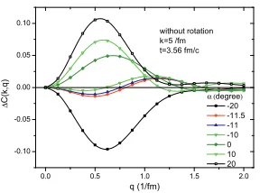
Figure 8.The Differential Correlation Function (DCF) at average pion wavenumber,k=5/fm and fluid dynamical evolution time,
t=3.56fm/c, as a function of the functions of momentum difference in the "out" directionq(in units of 1/fm). The DCF is evaluated in a frame rotated in the reaction plane, in the c.m. system by angleα. The figure shows the result where the rotation component of the velocity field is removed. The DCF shows a minimum in its integrated value overq, forα=−11 degrees. The shape of the DCF changes characteristically with the angleα. The "rotation-less" configuration is constructed in the fluid dynamical model, where the α=−11 degree symmetry angle is found. Unfortunately this is not possible experimentally, so the direction of the symmetry axes should be found with other methods, like global flow analysis and/or azimuthal HBT analysis.
The correlation function for the original fluid dynamical DCF with the rotation included is differ-ent from the one obtained from the rotation-less configuration, see Fig. 8. Atα =−11 degrees the correlation function is distinctly different from the rotation-less one and has a minimum of−0.085 at q=0.63/fm. Unfortunately this is not possible experimentally, so the direction of the symmetry axes should be found with other methods, like global flow analysis and/or azimuthal HBT analysis.
this deflection angle, and a minimum of−0.046 appears atq=0.76/fm. Thus, the magnitude of the DCF at the angle of the symmetry axis increased by nearly a factor of two.
Thus, the method is straightforward for symmetric emission objects, while for a general Global Collective Flow pattern one has to extract the shape symmetry axis with other methods. There are several methods for this task, and it takes some experimental tests, which of these methods are the most adequate for the task.
7 Conclusions
In this talk the importance of splitting flow fluctuations from Global Collective Flow was pointed out, and the methods of this separation were presented.
Such a separation will provide the possibility to separately study the Global Collective flow com-ponent, which includes novel new features not studied up to now, including rotation, turbulence, and Kelvin Helmholtz Instability.
As the measurement of directed flow is difficult due to its decreasing amplitude at increasing beam energies, alternative detection methods are presented, which are more sensitive to these processes.
We are looking forward that these new phenomena with the help of the suggested methods will open new ways of studying the properties of the Quark-gluon Plasma. Especially the transport prop-erties are the key features, as some of the new phenomena, like turbulence and the Kelvin Helmholtz Instability occur only in case of low viscosity.
References
[1] P.K. Kovtun, D.T. Son, A.O. Starinets, Phys. Rev. Lett94, 111601 (2005). [2] L.P. Csernai, J.I. Kapusta, Phys. Rev. Lett97, 152303 (2006).
[3] L.P. Csernai, invited talk at the Int. Nuclear Physics Conference,Firenze, Italy, June 2-7, 2013, in Press: EPJ Web of Conferences.
[4] V.K. Magas, L.P. Csernai and D.D. Strottman, Phys. Rev. C64014901 (2001). [5] V.K. Magas, L.P. Csernai and D.D. Strottman, Nucl. Phys. A712, 167 (2002). [6] L.P. Csernai, G. Eyyubova, V.K. Magas, Phys. Rev. C86, 024912 (2012). [7] The ALICE Collaborations, arXiv: 1306.4145 (2013).
[8] S. Floerchinger, U.A. Wiedemann, arXiv: 1311.7613v1 (2013). [9] L.P. Csernai, S. Velle, D.J. Wang, arXiv:1305.0396 (2013).
[10] F. Becattini, L.P. Csernai, D.J. Wang, Phys. Rev. C88, 034905 (2013). [11] B. Schenke, S.Y. Jeon, and C. Gale, Phys. Rev. C82, 014903 (2010). [12] P. Bozek, and I. Wyskiel, Phys. Rev. C81, 054902 (2010).
[13] A. Adil, and M. Gyulassy, Phys. Rev. C72, 034907 (2005).
[14] Iu. Karpenko, P. Huovinen, M. Bleicher, arXiv:1312.4160v1 (2013). [15] L.P. Csernai, J.I. Kapusta, Phys. Rev. D29, 2664 (1984).
[16] L.P. Csernai, J.I. Kapusta, Phys. Rev. D31, 2795 (1985).
[17] L.P. Csernai, V.K. Magas, H. Stöcker, and D.D. Strottman, Phys. Rev. C84, 024914 (2011). [18] L.P. Csernai, D.D. Strottman and C. Anderlik, Phys. Rev. C85, 054901 (2012).
[19] D.J. Wang, Z. Néda, and L.P. Csernai, Phys. Rev. C87, 024908 (2013) [20] L.P. Csernai, V.K. Magas, and D.J. Wang, Phys. Rev. C 87, 034906 (2013).


![Figure 6. The polarization of thecant polarization can be measured for particles at larger momenta,momenta in the transverse, [ Λ and Λ¯ particles observed in different directions and at different transversex, y] plane at the event-by-event c.m](https://thumb-us.123doks.com/thumbv2/123dok_us/8198776.1369443/8.482.65.411.83.224/polarization-polarization-transverse-particles-dierent-directions-dierent-transversex.webp)