Western University Western University
Scholarship@Western
Scholarship@Western
Electronic Thesis and Dissertation Repository
8-22-2014 12:00 AM
Perfect and Nearly Perfect Sampling of Work-conserving Queues
Perfect and Nearly Perfect Sampling of Work-conserving Queues
Yaofei Xiong
The University of Western Ontario Supervisor
Duncan J. Murdoch
The University of Western Ontario Joint Supervisor David A. Stanford
The University of Western Ontario
Graduate Program in Statistics and Actuarial Sciences
A thesis submitted in partial fulfillment of the requirements for the degree in Doctor of Philosophy
© Yaofei Xiong 2014
Follow this and additional works at: https://ir.lib.uwo.ca/etd
Part of the Other Statistics and Probability Commons
Recommended Citation Recommended Citation
Xiong, Yaofei, "Perfect and Nearly Perfect Sampling of Work-conserving Queues" (2014). Electronic Thesis and Dissertation Repository. 2313.
https://ir.lib.uwo.ca/etd/2313
This Dissertation/Thesis is brought to you for free and open access by Scholarship@Western. It has been accepted for inclusion in Electronic Thesis and Dissertation Repository by an authorized administrator of
(Thesis format: Monograph)
by
Yaofei Xiong
Graduate Program in Statistics and Actuarial Science
A thesis submitted in partial fulfillment
of the requirements for the degree of
Doctor of Philosophy
The School of Graduate and Postdoctoral Studies
The University of Western Ontario
London, Ontario, Canada
c
Abstract
We present sampling-based methods to treat work-conserving queueing systems. A vari-ety of models are studied. Besides the First Come First Served (FCFS) queues, many efforts are putted on the accumulating priority queue (APQ), where a customer accumulates priority linearly while waiting. APQs have Poisson arrivals, multi-class customers with corresponding service durations, and single or multiple servers.
Perfect sampling is an approach to draw a sample directly from the steady-state distribu-tion of a Markov chain without explicitly solving for it. Statistical inference can be conducted without initialization bias. If an error can be tolerated within some limit, i.e. the total varia-tion distance between the simulated draw and the stavaria-tionary distribuvaria-tion can be bounded by a specified number, then we get a so called “nearly” perfect sampling.
Coupling from the past (CFTP) is one approach to perfect sampling, but it usually requires a bounded state space. One strategy for perfect sampling on unbounded state spaces relies on construction of a reversible dominating process. If only the dominating property is guaranteed, then regenerative method (RM) becomes an alternative choice. In the case where neither the reversibility nor dominance hold, a nearly perfect sampling method will be proposed. It is a variant of dominated CFTP that we call the CFTP Block Absorption (CFTP-BA) method.
Time-varying queues with periodic Poisson arrivals are being considered in this thesis. It has been shown that a particular limiting distribution can be obtained for each point in time in the periodic cycle. Because there are no analytical solutions in closed forms, we explore perfect (or nearly perfect) sampling of these systems.
Keywords: Perfect sampling, Nearly perfect sampling, Work-conserving queues, Priori-ties, Homogeneous and time-varying queues
As I have reviewed my thesis, I am somehow surprised since I feel I have gained so much knowledge and have accomplished some findings through the Ph.D. program. But I know that I cannot achieve these only by myself and I owe a lot to other people.
My deepest gratitude will be expressed to my supervisors, Dr. Murdoch and Dr. Stanford, for their excellent guidance, patience and help. Dr. Murdoch led me into the area of perfect sampling hand in hand. He helped me to understand many complicated concepts and taught me a variety of practical techniques. As a queueing theory expert, Dr. Stanford’s experience and knowledge in this area made my sight broader.
I would like to thank Dr. Hao Yu and Dr. Qi-Ming He. After taking three courses in-structed by Dr. Yu, I learnt quite a lot in statistics. I got to know Dr. He in the conference CanQueue2013. He gave me constructive suggestions for the improvement of my research.
I would also like to thank my parents for their endless supporting and encouraging, which have powered me since I was born.
Finally, I would like to thank my wife, Lan Zhang, for her always cheering me up and standing by me in good or bad times.
Contents
Certificate of Examination ii
Abstract ii
Acknowlegements iii
List of Figures vii
List of Tables ix
1 Introduction 1
1.1 Accumulating priority queue . . . 1
1.2 Perfect sampling . . . 2
1.2.1 Coupling from the past . . . 3
1.2.2 Regenerative method . . . 3
1.2.3 Nearly perfect sampling . . . 4
1.3 Time-varying queues . . . 4
1.4 Problems to be solved . . . 5
1.5 Outline of this thesis . . . 6
2 Preliminaries 7 2.1 Notation and terminology . . . 7
2.2 Model specifications . . . 10
2.2.1 Accumulating priority queue . . . 10
2.2.2 Time-varying queues . . . 11
2.2.3 Queueing models to be treated . . . 12
2.3 CFTP related algorithms . . . 13
2.3.1 CFTP . . . 13
2.3.2 Multishift coupling . . . 14
2.3.3 Dominated CFTP . . . 15
2.3.4 Backward simulation of M/G/1 FCFS queue . . . 16
Solutions of M/G/1 FCFS queue . . . 16
Coupled processor sharing queue . . . 18
Randomly selected service duration . . . 18
Algorithm for backward simulation of M/G/1 FCFS queue . . . 20
2.4 Other perfect sampling algorithms . . . 22
Stationary waiting time in GI/G/1 FCFS queue . . . 24
Algorithm description . . . 25
2.5 Miscellaneous algorithms . . . 26
2.5.1 Ordinary simulation of GI/G/cFCFS queue with random assignment . 26 Stochastic upper bound in unfinished workload of multi-server queue . 27 Kiefer-Wolfowitz recursion . . . 27
Simulation algorithm for the RA model . . . 28
2.5.2 Time-varying Poisson process simulation . . . 28
Definition . . . 28
Simulation: Thinning method . . . 29
Simulation: Order statistics method . . . 29
Simulation: Inter-event time method . . . 30
2.5.3 Gaver-Stehfest inversion of LST . . . 31
3 Sampling homogeneous queues 32 3.1 Nearly perfect sampling of the GI/G/1 FCFS queue with heavy tail distribution inputs . . . 32
3.1.1 An example . . . 34
3.2 Ordinary simulation of APQ . . . 40
3.2.1 ΣKM/G K/1 APQ . . . 40
3.2.2 ΣKM/GK/cAPQ . . . 41
3.3 Perfect sampling ofΣKM/GK/1 APQ . . . 42
3.3.1 Class numbers of the randomly selected service durations . . . 43
3.3.2 Simulating backwards the coupledΣKM/G K/1 FCFS queue . . . 44
3.3.3 Restoring the APQ . . . 46
3.3.4 Examples . . . 47
3.4 Perfect sampling ofΣKM/G/cAPQ . . . 50
3.4.1 Using the regenerative method . . . 51
3.4.2 Using the dominated CFTP . . . 53
3.4.3 Algorithm to restore theΣKM/G/cAPQ . . . 55
3.5 Nearly Perfect sampling ofΣKM/G K/cAPQ . . . 60
3.5.1 Workload excess and carryover probability . . . 62
3.5.2 Upper bound of individual workload excess . . . 63
3.5.3 Upper bound of carryover probability . . . 66
The case of light tail service duration distributions . . . 67
The case of heavy tail service duration distributions . . . 69
3.5.4 Algorithm description . . . 70
3.5.5 Examples . . . 72
3.5.6 Algorithmic analysis of the nearly perfect sampling . . . 74
Distance to the target distribution . . . 76
Expected runtime . . . 76
Comparison with ordinary simulation . . . 78
4 Sampling time-varying queues 80
4.1 Perfect and nearly perfect sampling of Mt/Mt/1 FCFS queue . . . 83
4.1.1 Backwards simulating the M/M/1 FCFS queue with a specified num-ber of busy cycles . . . 83
4.1.2 Perfect sampling of Mt/Mt/1 FCFS queue with infµ(t)> supλ(s) . . . 83
4.1.3 Perfect sampling of the Mt/Mt/1 FCFS queue . . . 86
Sampling from the steady-state of the dominating process . . . 88
Algorithm for perfect sampling of the Mt/Mt/1 FCFS queue . . . 90
An example . . . 92
4.1.4 Nearly perfect sampling of Mt/Mt/1 FCFS queue . . . 92
Job excess and carryover probability . . . 94
Upper bound of the carryover probability . . . 99
Algorithm for nearly perfect sampling of the Mt/Mt/1 FCFS queue . . 102
An example . . . 103
4.2 Nearly perfect sampling of Mt/Mt/cFCFS queue . . . 103
4.2.1 Backwards simulating the M/M/cFCFS queue with specified number of busy cycles . . . 105
4.2.2 Simulating the potential departure events in each server . . . 106
4.2.3 Upper bound of the carryover probability . . . 108
4.2.4 Algorithm for nearly perfect sampling of the Mt/Mt/cFCFS queue . . . 111
4.3 Perfect sampling of Mt/G/1 queue . . . 112
4.3.1 The dominating process and its upper bound . . . 113
4.3.2 Algorithm for perfect sampling of Mt/G/1 FCFS queue . . . 114
4.3.3 Examples . . . 115
4.4 Quick extensions to other models . . . 116
4.4.1 Perfect sampling ofΣKMt/G/1 orΣKMt/GK/1 APQ . . . 117
4.4.2 Perfect sampling of Mt/G/cFCFS queue . . . 117
4.4.3 Perfect sampling ofΣKMt/G/cAPQ . . . 117
5 Conclusions and future work 118 5.1 Main contributions . . . 118
5.2 Future work . . . 120
Bibliography 122
Curriculum Vitae 126
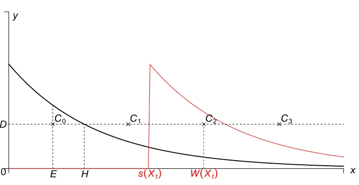
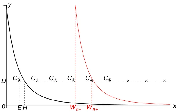
2.1 An illustration of multishift coupling. The solid black line is the standard Exp(µ) density; the red line is the density after shifting to an origin of s(Xt).
The valuesE and Dare selected at random as described in the text; pointsCi
and the valueW(Xt) are derived. . . 15
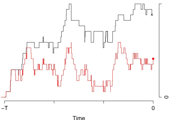
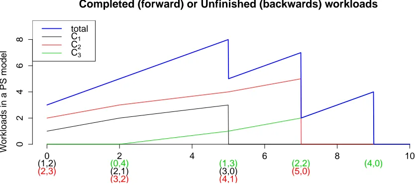
2.2 An illustration of dominated CFTP in a queueing system. These paths are the number of customers in the system. The black one is the dominator and the cross indicates a stationary draw of it at time 0. The red path belongs to the target chain and the point at time 0 is outputted as the steady-state draw of the system of interest. . . 17 2.3 Illustration of the time reversibility of the M/G/1 PS model. Denote by
(Com-pleted, Unfinished) the workload pair. Whent = 0 there are 2 customers (C1
andC2) with the pairs of (1,2) and (2,3). A new arrival (C3) att = 2 having
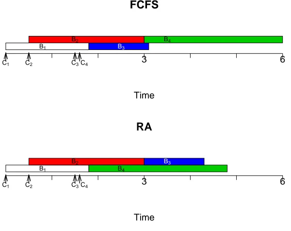
workload pair (0,4). . . 19 2.4 RA model is not the sample path upper bound of the simply coupled FCFS
queue. There are 4 customers (C1throughC4) arriving at times 0, 0.5, 1.5, and
1.6, whose service durations are 1.8, 2.5, 3, and 1.3 respectively. In the RA model, C1 and C4 are assigned to one server, andC2 and C3 to another. It is
obvious thatQ(5)> QRA(5). . . 26
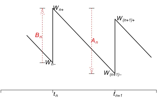
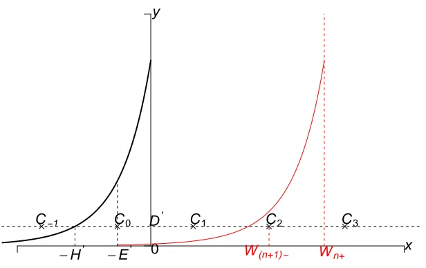
3.1 One transition of the unfinished workload fromWn− toW(n+1)− in the GI/G/1 FCFS queue, wheretnis the arrival instant of thenthcustomer. . . 33
3.2 Coupling the service durations in the first stage of transition with the Multishift Coupling method. . . 36 3.3 Coupling the inter-arrival times in the second stage of transition with the
Mul-tishift Coupling method. . . 37 3.4 A worse case of applying CFTP to the GI/G/1 FCFS queue which has Pareto
inter-arrival time and service duration distributions. The coalescence occurs in the third trial. . . 38 3.5 The e.c.d.f. from simulations of 1,000 independent draws of waiting times
in the GI/G/1 FCFS queue using the CFTP algorithm. Inter-arrival time and service duration both have Pareto distributions. Shaded areas are point-wise 95% confidence bands. . . 39 3.6 The e.c.d.f.’s from simulations of 1,000 independent draws of waiting times in
the APQ using the dominated CFTP algorithm, compared with the theoretical c.d.f.’s. Shaded areas are pointwise 95% confidence bands. . . 49
3.7 The e.c.d.f.’s from simulations of 1,000 independent draws of waiting times in the classical priority queue using the dominated CFTP algorithm, compared with the theoretical c.d.f.’s. Shaded areas are pointwise 95% confidence bands. 49 3.8 Totally idle periods of the coupled M/G/cFCFS andΣKM/GK/cAPQ, which
do not match in this sample realization. The horizontal bars are service dura-tions associated with customers. The gray bar corresponds to a class 1 customer and the black bar a class 2 customer. The upward arrows indicate the arrival instants. The class 2 customer arrives at time 1.5, and the class 1 customer at 1.6. The first departure occurs at 1.8. Under the FCFS discipline, the first busy cycle ends atτ1 =5. After applying the APQ discipline (b1 = 1,b2 = 0.5), the
workload excess (unfinished workload atτ1) interferes the second busy cycle. . 60
3.9 Blocks in the M/G/c FCFS queue. The gray rectangles are busy periods and blank ones are totally idle periods. A gray rectangle and a following blank one form a busy cycle. In this case, there are two busy cycles in blockC−1and two
ore more busy cycles inC−2. . . 62
3.10 The e.c.d.f.’s built of simulations of 1,000 independent draws of waiting times for each class in the APQ using the nearly perfect sampling method, where = 10−10. The legends of distributions correspond to the abbreviations assigned in
Table 3.3. . . 75
4.1 Construction of the dominating process of the Mt/Mt/1 queue. . . 88
4.2 Idle probabilities and expected numbers in the Mt/Mt/1 queue for one period.
100 points were chosen on it with equal intervals. 10,000 samples were drawn for each point. . . 93 4.3 Illustrations of the block scheme in the coupled M/M/1 FCFS queue. The gray
rectangles are busy periods and blank ones are idle periods.kis an integer. Plot (a) is the usual case. Plot (b) is a possible scenario, where there are some busy cycles between two successive blocks. . . 94 4.4 The upper bound of individual job excess introduced by constructing the
dom-inating process. Let CI
1 = (0,1], Q H
0 = 3, Q
H
1 = 4 and assume there are 5
arrival events (NA
1) and 4 potential departure events (N D
1). After rearranging
the instants of event occurrence according to the dominating process’ con-struction rule, L1 = 5. So the upper bound of job excess for this interval is
Ω1 = L1−QH1 = 1. . . 95
4.5 Idle probabilities and expected numbers in the Mt/Mt/1 queue for one period.
100 points were chosen on it with equal intervals. 10,000 samples were drawn for each point. . . 104 4.6 Average unfinished workloads and 95% confidence intervals (areas in gray
shadow) in two Mt/G/1 FCFS queues with Erlang and Pareto distributions of
the service durations. They involve 2 cycles and 100 points are drawn in each cycle. For each point we generate 10,000 samples. . . 116
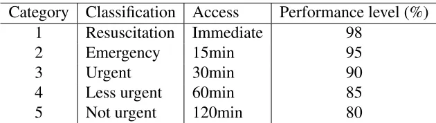
1.1 CTAS key performance indicators. Performance level (in percentage) is the compliance target for the proportion of that class’s patients that need to meet that standard. . . 2
2.1 Abbreviations . . . 8 2.2 Miscellaneous mathematical notations . . . 8 2.3 Queueing models to be treated with perfect (or nearly perfect) sampling . . . . 12
3.1 Numerical results of the 1,000 simulations of the GI/G/1 FCFS queue . . . 39 3.2 Variable definitions for Algorithm 1 . . . 46 3.3 Values ofm−1with different service distribution assumptions. . . 74
3.4 Estimates and 95% confidence interval of waiting times of class 1 customers with 1,000 samples, where =10−10. . . 74 3.5 Estimates and 95% confidence interval of waiting times of class 2 customers
with 1,000 samples, where =10−10. . . 75
Chapter 1
Introduction
This thesis presents perfect (or nearly perfect) sampling of some work-conserving queueing
systems with homogeneous or time-varying inputs. For the homogeneous queues, we focus
on the analysis of accumulating priority queues (APQ) to demonstrate our methods concretely.
For the time-varying queues, we study the quasi-birth and death processes and periodic Poisson
arrival queues under the First Come First Served (FCFS) discipline.
In this chapter, background and motivation are introduced, key methods mentioned and
contents of this thesis outlined.
1.1
Accumulating priority queue
The accumulating priority queue was introduced as the “time-dependent priority queue” by
Kleinrock [31]. It is a queue in which customers accumulate priority as a linear function of
their time in the queue: the higher the priority class of a customer, the greater the rate at
which that customer accumulates priority. When the server becomes free, the customer with
the highest priority accumulated to that instant, if any, is the one that is selected by the server.
Whereas Kleinrock [31] derived a set of recursive formulae for the average waiting time for
the different classes, Stanford et al. [54] extended Kleinrock’s analysis to derive the Laplace-Stieltjes Transform (LST) of the stationary waiting time distribution for each class in the
Pois-son arrival, general service duration and single-server case.
In [54], the APQ was motivated by applications in health care. Generally, patients are
classified according to some acuity rating system, such as the Canadian Triage and Acuity
Scale (CTAS) [11], as shown in Table 1.1 with some Key Performance Indicators (KPIs). It is
not reasonable to assign absolute priorities to patients with relatively different service require-ments, where a patient of lower priority classes can be overtaken many times by those of higher
priority, without any priority being accrued while the patient waits with possibly deteriorating
Category Classification Access Performance level (%)
1 Resuscitation Immediate 98
2 Emergency 15min 95
3 Urgent 30min 90
4 Less urgent 60min 85
5 Not urgent 120min 80
Table 1.1: CTAS key performance indicators. Performance level (in percentage) is the compli-ance target for the proportion of that class’s patients that need to meet that standard.
health. The APQ rectifies this weakness by allowing waiting customers to earn priority while waiting, at a rate that depends upon their priority class. In this way, low priority customers
eventually earn enough credit to be served ahead of recently-arrived high priority ones.
Based on Stanford et al. [54], Sharif et al. [50] considered the multi-server case, with the additional requirement that the service durations be identically and exponentially
dis-tributed. Then numerical inversions of Laplace transforms are performed with the
Gaver-Stehfest method (c.f. Abate and Whitt [3], Gaver [16] and Gaver-Stehfest [55]) to calculate the
probabilities of waiting times exceeding some limits. At present, no equivalent analytical
re-sult exists for more general cases, therefore sampling-based methods are strong candidates.
1.2
Perfect sampling
In Markov Chain Monte Carlo (MCMC), a common approach to generate draws from a
“steady-state” distribution of a Markov chain is to sample from an arbitrary starting point, then discard the first so many draws. This discarding is done in order to remove any possible bias due to the
initial conditions at the start of the simulation; such bias is sometimes referred to as
“initial-ization bias” [37, p. 287] and the period of time discarded is referred to as the “burn in”. The
burn-in period is chosen to be long enough that the remaining draws are close to the
steady-state distribution. Steady-steady-state properties are estimated using the remaining draws. A practical
difficulty is that for most chains the appropriate burn-in time is unknown.
Perfect sampling is an approach to draw a sample directly from the steady-state distribution
without explicitly solving for it. It is also called “exact sampling”, “perfect simulation” or
“exact simulation”. With perfect sampling, the burn-in time is not an issue.
The first well-known perfect sampling algorithm is commonly referred to as Coupling From
The Past (CFTP), proposed by Propp and Wilson [45]. Actually, Asmussen et al. [9] had
1.2. Perfect sampling 3
1.2.1
Coupling from the past
Conceptually, an infinitely long run of the chain is simulated as starting in the indefinite past,
so that the draw at time 0 is in steady state. The original CFTP by Propp and Wilson [45]
mainly considers sampling steady-state draw for finite-state Markov chains. If one were to run
coupled chains from all possible states at a finite time in the past, and if all of them result in the
same output at time 0 (i.e., they coalesce by time 0), then this value will be identical to what
would be achieved in any longer run, so its distribution must be the steady-state distribution.
To facilitate the implementation of algorithms, Read Once Coupling From The Past (ROCFTP)
was presented by Wilson [58], where the random variables which drive the coupled Markov
chains are used only once.
People might give up when encountering a long run of CFTP, and introduce “user-impatience bias” (named by Fill [15]). Fill invented a “rejection sampling” algorithm for perfect sampling.
Starting from a given time in the future, firstly it performs simulation backwards from an
arbi-trary state and ends at time 0. Then it goes forward running chains from all possible states with
the random numbers generated in the first step until the originally given time. Finally it accepts
(or rejects) the state at time 0 if all chains coalesce (or do not). This method is nice since it
avoids impatience bias, but it requires simulation of the time-reversal of the chain which is hard
to achieve.
Wilson [57] proposed Multishift Coupling for families of location shifted distributions,
which allows efficient coupling of Markov chains with continuous state spaces. This allows coalescence to be detected by the coalescence of minimal and maximal states. It is a
“mono-tone” coupling, in the sense that the ordering of states is preserved in each transition.
“Dominating coupling” by Kendall and Møller [29] is an important extension of CFTP. We call this extended version as dominated CFTP. It enables coupling Markov chains with
unbounded state spaces by reducing the number of past chains that need to be simulated. For
situations with a natural (partial) ordering on the state space, simpler chains that dominate the
target ones are constructed and simulated backwards from time zero. When going forward, the
target chain only need to be simulated from values lying below the dominators. The
construc-tion of the reversible dominating chain is the key in this method.
1.2.2
Regenerative method
The workload or queue length of a stable queueing system can be treated as a regenerative
process. The regenerative points are the instants with a customer entering an empty system.
The stopping time is the length of a conventional busy cycle (a busy period followed by an idle
As shown by Sigman [52], Asmussen et al. [9] and Asmussen and Glynn [6, p. 420], we
can simulate exactly from the stationary distribution of the queueing system if we can simulate
exactly from the equilibrium distribution of a busy cycle length, i.e. the distribution of the
residual of a randomly selected busy cycle.
The outstanding advantage of this method is quite appealing: it does not need a reversible
chain. But its drawback is that the expected runtime is infinite (see Proposition 2.4.2). In
practice, this algorithm will always finish in finite time, but occasionally will take a very long
time to do so.
1.2.3
Nearly perfect sampling
Truly perfect sampling is hard to achieve due to high dimensions or the difficulty in reversible dominating chain construction. Fortunately, in the queueing context, when the stable queue can
be treated as a stochastic process with unfinished workload (or queue length) as the variable,
the high dimension issues can be avoided.
Nearly perfect sampling can be considered as an asymptotic perfect sampling with well
specified distance to the target distribution. The quantitative assessment of it makes this method valuable. As shown by Asmussen and Glynn [6, p. 100], and Zeifman et al. [60], the upper
bound of differences between the first moments of the transient distributed samples and the stationary ones can be controlled to be guaranteed to be within an arbitrary distance.
In this thesis, we define the difference as the total variation distance [37, p. 47] between the simulated draw and the stationary distribution. Using our CFTP Block Absorption (CFTP-BA)
method (Section 3.5), we can simulate samples guaranteed to be within a 10−10 total variation
distance of the stationary distribution in a few seconds of computing time.
1.3
Time-varying queues
Time-varying queueing models are more realistic, but they are not usually mathematically
tractable (Ross [49, p. 697]). As noted by Margolius [41], computational methods and
approx-imation techniques involved in time-varying queueing problems have long been regarded as
challenging. The time-varying ingredients can exist in the arrival processes, service durations,
or the number of servers, as mentioned by Alfa and Margolius [4].
Generally, it is acceptable that the time-dependent stochastic processes take some periodic
patterns. As for the periodic Poisson arrival single-server queue with general service duration,
Hasofer [22] showed that the LST of its virtual waiting time (i.e. unfinished workload) is
1.4. Problems to be solved 5
time at a given time does have a limiting distribution and has the same period length as the
arrival rate does.
Asmussen and Thorisson [8] extended the context to more general cases, where the
inter-arrival times and service durations both depend on the inter-arrival instant with some periodic
pat-tern. They proved that with more conditions (such as Harris ergodicity of the phase
parame-ter which the inparame-ter-arrival time and service duration depend on), the virtual waiting time and
queue length also have time dependent limiting distributions in periodic patterns. Due to the
complexity of time-varying systems, only asymptotic solutions have been developed, and this has happened gradually over recent decades.
Time-varying quasi-birth and death processes have been frequently studied for the
tran-sient or periodic solutions. By assuming some state (generally idle) at time 0, Zhang [61]
and Margolius [40] figured out the transient distributions of queue length in the single-server and multi-server cases respectively. Zeifman et al. [60] approximated the limiting mean value
(expected queue length at some given time) of the single-server model with the transient
dis-tribution by restricting their difference to some controllable extent. The asymptotic periodic solutions for single-server and multi-server models were achieved in Margolius [41], where
distributions and moments were presented in terms of integral equations.
In this thesis, queueing systems are generally presumed to be homogeneous ones unless
they are specifically pointed out as time-varying.
1.4
Problems to be solved
Analytically intractable models, such as Poisson arrival, multi-server multi-class APQs with
differently distributed service durations, and time-varying APQs with periodic Poisson arrivals, are good candidates to apply perfect (or nearly perfect) sampling.
For partly solved models (e.g. results of the time-varying queues with periodic Poisson arrivals by Lemoine [36] only present the moments of some statistics such as workload and
waiting time), the perfect sampling method provides direct solutions for the probability mass of
the queue length and tail probabilities in a simulation based way without having to approximate
based upon moment-based methods (c.f. Provost et al. [46]).
For problems with solutions in LST forms (like Hasofer [22], Stanford et al. [54] and Sharif
et al. [50]), applications of these methods are also validated in the sense that they provide
alternative and comparable solutions to the numerically inverted LST ones. As noted by Abate
and Whitt [3], the commonly used inversion, by Gaver [16] and Stehfest [55], only has limited
accuracy, restricted by the number of transform evaluations and computer system precision
In the work-conserving context, these methods are adaptive automatically to any priority
disciplines specified, because they do not affect the computation of the tail of the infinitely long run. More specifically, as for the work-conserving single server queue, the unfinished
workload path stays invariant no matter what priority disciplines are applied.
1.5
Outline of this thesis
As noted earlier, the dominated CFTP achieves perfect sampling of the Markov chains with
unbounded state within finite expected runtime, so it is the the preferred choice in what follows.
But when the reversible dominating process is hard to construct, we resort to the regenerative
method or nearly perfect sampling by CFTP Block Absorption (CFTP-BA).
In Chapter 2, notations and models are specified, and related existing algorithms are intro-duced as components for addressing new problems.
These algorithms are: 1) CFTP related (original CFTP, multishift coupler, and reversion
of single-server queue with Poisson arrivals); 2) other perfect sampling methods (regenerative
method and a special case for general single-server queue); 3) miscellaneous ones (ordinary
simulation of multi-server queue with Random Assignment (RA), time-varying Poisson
pro-cess simulation, and Gaver-Stehfest algorithm for numerical inverse of LST).
Chapter 3 deals with homogeneous queues with single or multiple servers. After applying
the CFTP to a single-server queue with heavy tail inter-arrival time and service duration, we
go to APQs. Perfect sampling methods are applied to various queueing models with Poisson arrivals and general service durations. When the service distributions differ among different classes, the reordering of service durations will affect the distribution of the busy period in the multi-server case. The new method we call CFTP-BA will be introduced and applied.
Chapter 4 explores time-varying queueing systems. Periodic Poisson arrivals are assumed,
and the service durations could be periodically time-dependent exponential or homogeneous
general ones. We focus on the FCFS discipline and briefly describe quick extensions to some
APQ models.
Results and contributions are summarized in Chapter 5. Some related new topics will be
Chapter 2
Preliminaries
2.1
Notation and terminology
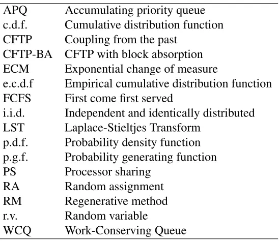
For the sake of clearness and consistency, abbreviations and miscellaneous mathematical
nota-tions are shown in Tables 2.1 and 2.2 respectively.
For different queueing systems, Kendall’s notation (c.f. [28]) is used as the standard classi-fier. Since we assume an unlimited waiting room and infinitely large population of customers,
and specify the discipline additionally, the three-part code (a/b/c) is enough. When it is not
explicitly specified, it is presumed there are infinite waiting room and population of customers. The first letter indicates inter-arrival time distribution, the second one service duration
distribu-tion, and the third one the number of servers. Conventionally, “M” stands for the exponential
distribution, and “G” for an unspecified “general” distribution.
In this thesis, it is assumed that the inter-arrival times are independent (corresponding to
notation “GI”), service durations independent, and the service durations are also independent
of the inter-arrival times.
In the priority queueing systems, in the light of Stanford [53], we introduce notation “ΣK”
pointing out that the arrival process is a superposition ofKindependent streams. If the classes
of customers might have different distributions of service durations, subscriptKis added to the service code. E.g. ΣKM/MK/1 stands for a single-server priority queue with K (≥ 2) classes
of customers arriving in Poisson processes, and each class has its own exponential service
duration distribution.
As for the time-varying queues, as noted in some recent papers (c.f. Margolius [40] and
Zeifman et al. [60]), subscripttimplies that the inter-arrival time or service duration’s
distribu-tions are time dependent. For instance, the notation Mt/Mt/1 indicates that it is a single-server
queue with time-varying Poisson arrival and the service duration is exponential with time
vary-ing rate.
APQ Accumulating priority queue c.d.f. Cumulative distribution function CFTP Coupling from the past
CFTP-BA CFTP with block absorption ECM Exponential change of measure
e.c.d.f Empirical cumulative distribution function FCFS First come first served
i.i.d. Independent and identically distributed LST Laplace-Stieltjes Transform
p.d.f. Probability density function p.g.f. Probability generating function
PS Processor sharing
RA Random assignment
RM Regenerative method
r.v. Random variable
WCQ Work-Conserving Queue
Table 2.1: Abbreviations
Z Integers: 0,±1,±2,. . . N Positive integers: 1,2,. . .
R Real numbers
D
= Identically distributed
D
≥ Large or equal statistically
=so Stochastically equal
≥so Stochastically larger or equal
⊥ Independent
∃ Exists
∀ For all
3
−− Such that
dxe The smallest integer which is no less than x bxc The largest integer which is no greater thanx
(x)+ The non-negative truncated value of x, i.e. xifx>0 or 0 if x≤ 0 Exp(λ) Exponential distribution with rate ofλ
Geom(p) Geometric distribution with success probability of p, Poi(λ) Poisson distribution with arrival rate ofλ
Unif(0,1) Uniform distribution on (0,1)
NB(r,p) Negative binomial distribution with number of successesrand success probability p
2.1. Notation and terminology 9
Busy period in multi-server queues The busy period in multi-server queues is defined as a
duration started at the arrival instant when the arriving customer finds an empty system, and
after that for the first time terminated at the departure instant, when the departing customer
leaves behind no busy servers. See Wiens [56] and Ghahramani [17]. The latter called it “partial busy period”.
Totally idle period in multi-server queues It is the duration in the multi-server system when
all servers are idle.
Reversibility A stochastic processX(t) is reversible [27, p. 5] if (X(t1),X(t2), . . . ,X(tn)) has
the same distribution as (X(τ−t1),X(τ−t2), . . . ,X(τ−tn)) for allt1,t2, . . . ,tn, τ∈R.
In a word, when going forward or backwards along this process in time, what we see are
statistically equivalent. So we also call it time reversible.
Light/Heavy tail distributions We define light tail distribution as those which decay at an
exponential rate or faster (c.f. Asmussen and Glynn [6, p. 163]). In queueing studies, usually
the distributions of interest have positive support (0,∞). So a distribution G(·) of light tail requires that there exists >0 such that
Z ∞
0
exdG(x)< ∞.
We consider heavy tail distributions as those which have super-exponential tails, i.e.R0∞exdG(x)=
∞for all >0 [5, p. 412].
Total variation distance The total variation distance between two probability distributionsν1
andν2onΩis defined by
||ν1−ν2||T V =max
E⊂Ω
|ν1(E)−ν2(E)|.
It can be computed as
||ν1−ν2||T V =
1 2
X
x∈Ω
|ν1(x)−ν2(x)|. (2.1)
A brief explanation is presented as follows. Let E = {x : ν1(x) ≥ ν2(x)}, then||ν1− ν2||T V =
P
x∈E(ν1(x)−ν2(x)). Please note that
X
x∈E
(ν1(x)−ν2(x))=
X
x∈Ec
(ν2(x)−ν1(x))=
1 2
X
x∈Ω
|ν1(x)−ν2(x)|,
sinceν1(Ω)=ν2(Ω)= 1. Therefore equation (2.1) holds.
2.2
Model specifications
Non-preemptive work-conserving queue We define a non-preemptive work-conserving queue
discipline (NPWCQ) to be one in which the work requirements of customers are unaltered by the passage of time and the server never idles when there is work to be done. Customers that
enter service remain in service until completion. This definition adds the lack of preemption to
the definitions given by Gross and Harris [19, p. 299], and Kleinrock [33, p. 113]. This means,
in particular, that customers do not renege. When there exists an idle server, a customer’s
ser-vice startes upon arrival. Otherwise, the customer joins a pooled queue and will be selected to
go into service according to some discipline when any server becomes available.
For writing convenience, in this thesis we use “work-conserving queue” (WCQ) to stand
for NPWCQ.
2.2.1
Accumulating priority queue
This discipline was first proposed by Kleinrock [31] and was termed as “time-dependent
prior-ity queue”. According to Stanford et al. [54], the specification of the APQ is described below.
Assume there are K ∈ N(K ≥ 2) classes of customers, and one orc(≥ 2) servers in the system. Each class of customers arrives independently in a Poisson process with rate λi, i =
1, . . . ,K.
For classicustomers, the priority accumulates linearly at ratebi, i.e. if a customer of class
iarrived at timetand is still in the system at timet0, then its priority at timet0isbi(t0−t), and
b1 > b2 > · · · > bK. When any server is available, the next customer to be served is the one
with the greatest priority at that instant. This is a non-preemptive system.
Let Abe the inter-arrival time, whose c.d.f. isA(x), of two successive customers, andA(i)
be that of classicustomers. According to the aggregation and branching property (c.f. Conway
et al. [13, p. 143]) of the Poisson process, it follows
A∼Exp(λ),A(i) ∼Exp(λi), andA= min{A(i),i= 1, . . . ,K}
whereλ=PK
i=1λi. And a customer is classified as classiwith probability of λλi.
Let B(i)be the service duration of classicustomers with c.d.f. Gi(x), and Bbe the generic
service duration with c.d.f.G(x) under the FCFS discipline, thenGis a mixture ofGi, i.e.
G(x)=
K
X
i=1
λi
λGi(x). (2.2)
2.2. Model specifications 11
of a randomly selected busy period of the M/G/1 FCFS queue) do exist, we assume
E
B(i)2
<∞.
It follows thatE
B(i) <∞, and
E
B2 <∞. Denote the corresponding service rates as
µi =
1
E B(i),
andµ= 1
E(B).
In the single-server scenario, the occupancies are
ρi =
λi
µi
, andρ = λ
µ.
In the multi-server scenario
ρi =
λi cµi
, andρ = λ
cµ.
It is easy to verify that
ρ=
K
X
i=1
ρi,
since the mean service duration is the weighted average of those of all classes
1
µ =
K
X
i=1
λi λ 1 µi ⇒ λ µ = K X
i=1
λi
µi
⇔ρ =
K
X
i=1
ρi.
To ensure the system is stable [32, p. 19], it must be assumed that
ρ <1,
which guarantees that the system empties occasionally, with probability 1.
2.2.2
Time-varying queues
In this thesis we also consider some time-varying queues, specifically those with periodic
ar-rival and service processes. Without loss of generality, we assume the period length is 1.
According to Asmussen and Thorisson [8], the periodic single-server queue can be defined
as follows: at the arrival instant of thenthcustomer, say at timet, the service duration B n and
the inter-arrival time,An, to the next arrival, are drawn according to distributions with c.d.f.Gθ
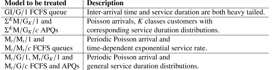
Model to be treated Description
GI/G/1 FCFS queue Inter-arrival time and service duration are both heavy tailed.
ΣKM/G
K/1 and Poisson arrivals,K classes customers with
ΣK
M/GK/cAPQs corresponding service duration distributions.
Mt/Mt/1 and Periodic Poisson arrival and
Mt/Mt/cFCFS queues time-dependent exponential service rate.
Mt/G/1, Mt/GK/1 and Periodic Poisson arrival and
Mt/G/cFCFS and APQs general service duration distributions.
Table 2.3: Queueing models to be treated with perfect (or nearly perfect) sampling
For the time-varying quasi-birth and death processes (denoted as Mt/Mt/1 or Mt/Mt/c
FCFS queues), they have time-dependent Poisson arrival rates and “time-dependent
exponen-tial service rates” [40]. Letλ(t) ≥ 0 andµ(t) ≥ 0 be the arrival and service rates, which have
period length of 1, i.e.
λ(t)=λ(t+1) andµ(t)=µ(t+1),∀t∈R.
Bothλ(t) > 0 andµ(t) > 0 except at discrete points, so their integrals are strictly increasing.
Then
Aθ1(x) = 1−e−
Rx
0 λ(θ1+s)ds,
Gθ2(x) = 1−e
−Rx
0 µ(θ2+s)ds,
where θ1 is the instant of arrival, and θ2 the instant of entry into service. Under the FCFS
discipline,θ2can be determined with the unfinished workload seen atθ1.
In the priority systems, we assume all classes of customers arrive as independent periodic Poisson processes with
λ(t)=
K
X
i=1
λi(t), ∀t∈R.
Service durations have homogeneous distributions, because the entry into service times are
affected by the priority discipline, it is hard to determine them at the arrival instants. So these models are denoted asΣKM
t/GK/1 orΣKMt/G/c.
2.2.3
Queueing models to be treated
With notations and models being specified above, we summarize the models to be treated with
2.3. CFTPrelated algorithms 13
2.3
CFTP related algorithms
2.3.1
CFTP
The CFTP algorithm was introduced by Propp and Wilson [45]. It allows perfect sampling of
an ergodic Markov chain. It can be applied to bounded and continuous state space chains.
For the refined algorithms and brief proofs of CFTP, see Murdoch and Takahara [43] and Asmussen and Glynn [6, p. 120].
We will describe it for the case of a finite state space labelled as 1,2, . . . ,n. Denote byXt
the ergodic Markov chain. Suppose that it can be simulated using a recursive formulation
Xt+1= φ(Xt,Ut+1), t∈Z, (2.3)
whereUt+1are i.i.d. from some known distribution, andφis a deterministic function.
In the CFTP context, let X(τm,j)
t be the Markov chain starting from time τm with state j,
whereτm<0,m=0,1, . . ., and j= 1,2, . . . ,n. We will usually setτm =−2mT0, whereT0∈N
is a constant.
The algorithm can be performed in the following way:
(1) Run the initial trial (i.e. m=0 andτ0 = −T0) to detect the coalescence.
Generate i.i.d. Ut (t = τ0 +1, τ0+ 2, . . . ,0). Then update X(
τ0,j)
t (j = 1,2, . . . ,n) with
formula (2.3) and these random numbers.
IfX(τ0,j)
0 = X
(τ0)
0 ,∀j = 1,2, . . . ,n, i.e. they have coalesced by time 0, then output X (τ0)
0 as
the steady-state draw. Otherwise, go to step (2).
(2) Conduct extra trials (i.e. m≥1 andτm=−2mT0) starting withm=1:
Generate extra i.i.d.Ut(t= τm+1, τm+2, . . . , τm−1). Then updateX(tτm,j)(j=1,2, . . . ,n)
with formula (2.3) andUt (t= τm+1, τm+2, . . . ,0).
IfX(τm,j)
0 = X
(τm)
0 ,∀j=1,2, . . . ,n, then stop repeating and outputX (τm)
0 as the steady-state
draw. Or else increasemby 1 and repeat this step.
Remark
(1) In the extra trials of detecting coalescence, the random variables generated in previous trials
must be reused.
(2) The choice ofT0depends on the characteristics of the system. E.g. in the queueing system,
and it tends to take a long run to return zero, so we prefer a relatively largeT0, which allows a
greater chance of coalescence to occur.
(3) τm could take−2mT0 (m ≥ 1), −2mT0, or other values. The geometric scheme accelerates
coalescence in the extra trials.
(4) The runtime is finite due to the “geometric trial argument” (see proposition 8.1 by Asmussen
and Glynn [6, p. 122]).
2.3.2
Multishift coupling
Before explaining this algorithm, we state the concept of monotonicity (see Murdoch and
Taka-hara [43] and Propp and Wilson [45]). An update function is said to be monotonic if it preserves
the partial order in the state space, i.e. X Y impliesφ(X,u) φ(Y,u) for allu. With
mono-tonicity, only maximal and minimal elements need to be followed, as all others are sandwiched
between them.
Here “” represents the partial order relation. IfXandY are scalar values, then the partial
order could be the usual numerical order. When they are vectors, we can define a
component-wise partial order asX Y ifX(i)≤ Y(i) for alli.
The choice of update function φ(·,·) is crucial. It must be chosen so that updates coalesce
and coalescence can be detected, which is not always easy. For example, we need to simulate
shifted exponential completion instants W when simulating the completion of service for an
individual who starts service at times(Xt). A simple choice would be to simulateE ∼Exp(µ),
whose c.d.f. has the form 1−e−µx,x > 0, and setW(Xt) = s(Xt)+E, but then different s(Xt)
values would always lead to differentW(Xt) values.
Wilson [57] proposed Multishift Coupling for families of location shifted distributions,
and we can use this coupling to handle unimodal distributions. Continuing with the example
above, for s(Xt) = 0 we set W = E, but use the following construction (see Figure 2.1) for
other values. After obtaining E, we sampleU ∼ Unif(0,1) and multiply it by the density at
E to obtain D = Uµexp(−µE) and the point C0 = (E,D). We then compute H by setting D =µexp(−µH), and replicateC0 asCn = (E+nH,D),n∈Z(shown as asterisks in the plot).
For any value of s(Xt), exactly one of these points lies under the shifted density; we use that
point’s horizontal coordinate asW(Xt).
By construction,W(Xt) takes on a discrete lattice of values as s(Xt) varies. This is a
mono-tone coupling, i.e. it preserves monotonicity, in the sense that the ordering of s(Xt) values is
preserved in the correspondingW(Xt) values, and our simulations from multiple starting
val-ues will result in coalescence whens(Xt) falls in a sufficiently small interval. E.g. as shown in
2.3. CFTPrelated algorithms 15
0 x
y
s(Xt)
E
C0 C1 C2 C3
D
H W(Xt)
Figure 2.1: An illustration of multishift coupling. The solid black line is the standard Exp(µ) density; the red line is the density after shifting to an origin of s(Xt). The valuesE andDare
selected at random as described in the text; pointsCiand the valueW(Xt) are derived.
With this method, we can perform coupling in a continuous state space. Uncountably many
chains will coalesce to a finite number of different states at the first transition.
2.3.3
Dominated CFTP
As mentioned in Section 2.3.1, ordinary CFTP is only easily applied to bounded state chains.
However, in queueing models, the state space (e.g. unfinished workload or queue length) is
usually unbounded, so we need to upgrade our method. The dominated CFTP was introduced
by Kendall and Møller [29]. Its basic idea is to reduce the number of chains to be simulated. We want to sample a steady-state draw from{Xt}t∈R, but it is too complex to implement.
Sup-pose we can construct a dominating process{Yt}t∈R, which dominates our target process in the
following sense. Let be a partial order on the common state space ofXt andYt. We say Yt
dominatesXtif for anyt0whereXt0 Yt0 we haveXt Yt for allt≥ t0with probability one, i.e.
sample paths ofXtare caught below sample paths ofYt. Assume we know how to sample from
the dominating process and achieve the backward simulation. So we can use it as an upper
bound to conduct the ordinary CFTP, and the unbounded problem is solved.
It is quite appealing to apply dominated CFTP for queueing systems, because in many
within finite time.
Proposition 2.3.1 Suppose we have a coupled simulation of two stable queues, denoted by
{Xt}t∈R and{Yt}t∈R. We assume the following:
1. Both are real-valued, with 0 as a minimal state.
2. Y0is a draw from the steady-state distribution of Yt.
3. We can simulate Yt backwards in time, and find an instant Ta ≤0at which YTa =0.
4. Yt dominates Xt in the usual ordering for real numbers.
Then in the coupled simulation of Xt started from XTa = 0, X0 will be a draw from the
steady-state distribution of Xt.
Proof Start both chains in state 0 at time t0 < 0. Then Yt ≥ Xt for all t ≥ t0 by dominance.
Lett0 → −∞; then both X0and Y0 tend to their steady-state distributions. The coupling only
allows one possible path for Xt on [Ta,0], so X0 as constructed above must be a steady-state
draw.
Figure 2.2 illustrates the dominated CFTP in a queueing system.
2.3.4
Backward simulation of M
/
G
/
1
FCFS queue
As mentioned before, the key of dominated CFTP is to find a dominating chain and we are able to simulate the reversal. Generally, the reversibility is harder to achieve than dominance. One
feasible way is to construct a coupled time reversible chain.
It is well-known that the output process of an ergodic M/M/1 FCFS queue is time reversible
(Ross [49, p. 399]), since it is a birth and death process, which is time reversible. But the
M/G/1 FCFS queue is not.
Sigman [51] presented a method to simulate the M/G/1 FCFS queue backwards, based on
Theorem 5.7.6 by Ross [48, p. 280]. The coupled M/G/1 Processor Sharing (PS) queue was
introduced, whose output is also a Poisson process with the same rate as the arrivals.
Solutions of M/G/1FCFS queue
Recall that, in the M/G/1 FCFS queue, according to the Pollaczek-Khintchine formula (see
Kleinrock [32, p. 200]), the stationary unfinished workload has LST as
e
W(s)= s(1−ρ)
s−λ+λeB(s)
2.3. CFTPrelated algorithms 17
Time
−T 0
0
Figure 2.2: An illustration of dominated CFTP in a queueing system. These paths are the number of customers in the system. The black one is the dominator and the cross indicates a stationary draw of it at time 0. The red path belongs to the target chain and the point at time 0 is outputted as the steady-state draw of the system of interest.
whereρ= λ/µis the occupancy rate, andBe(s) the LST of service durationB. It can be written
as
e
W(s)= 1−ρ 1−ρ
1−eB(s)
s/µ
=
1−ρ
1−ρeB∗(s)
,
where
e
B∗(s)= 1−eB(s)
s/µ . (2.4)
Equation (2.4) is the LST of the equilibrium distribution of the service duration.
It is clear that
p
1−(1− p)z
is the p.g.f. of Geometric distribution with success probability of p. Therefore the stationary
unfinished workload is a compound Geometric distribution, and it can be represented as
W =
Q
X
i=1
Yi, (2.5)
the service duration and they are i.i.d.’s. IfQ=0, thenW =0.
LetT be the length of busy period of M/G/1 queue, andTe(s) its LST. It is well known (e.g.
Kleinrock [32, p. 213-214]) that
e
T(s)= eB
s+λ−λTe(s)
, (2.6)
E(T)= E(B)
1−ρ, andE(T
2
)= E(B
2)
(1−ρ)3. (2.7)
Coupled processor sharing queue
The Processor Sharing (PS) discipline referred in this thesis is the round-robin scheduling
algorithm (Kleinrock [33, p. 166] ), with all quanta of the service capacity shrinking to zero.
It is a single-server system. Any customer’s service starts immediately at the arriving instant,
and all of them sojourning in the system share the capacity of the server equally.
The M/G/1 PS model and the M/G/1 FCFS queue are coupled in the way that they are
fed with the same arrival instants and service requirements. Since workload in a single-server queue is invariant under all conserving disciplines, the sample paths of unfinished
work-load in the coupled PS model and the FCFS queue are exactly the same.
LetQ(t) be the number of customers in the PS model, andY1(t), . . . ,YQ(t)(t) the
correspond-ing completed (or unfinished) workloads of the customers. It is shown by Ross [48, p. 280]
that it has stationary distribution in the form as
(Q,Y1, . . . ,YQ),
where Q and Yi are the same as those in equation (2.5), and its departure process is also a
Poisson process with rate of the arrival one (λ). Define Y~(t) = (Y(1)(t), . . . ,Y(Q(t))(t)) as the
ascending ordered vector of completed workloads, then {Q(t), ~Y(t)} is time reversible. When
looking forward, they are completed workloads. If looking backwards in time, they become
unfinished workloads, as illustrated in Figure 2.3.
Randomly selected service duration
For a stationary M/G/1 PS queue, we check its state at time 0. Due to stationarity, the state at
time 0 has the same distribution as the state at a randomly selected point in time, assuming the
selection is independent of the process. LetX denote the length of a selected service duration,
Y the remaining time andZ the age.
dura-2.3. CFTPrelated algorithms 19
Completed (forward) or Unfinished (backwards) workloads
W
or
kloads in a PS model
0 2 4 6 8 10
0
2
4
6
8
(1,2)
(2,3) (0,4)(2,1) (3,2)
(1,3) (3,0) (4,1)
(2,2)
(5,0) (4,0)
total C1
C2
C3
Figure 2.3: Illustration of the time reversibility of the M/G/1 PS model. Denote by (Com-pleted, Unfinished) the workload pair. Whent = 0 there are 2 customers (C1andC2) with the
pairs of (1,2) and (2,3). A new arrival (C3) att=2 having workload pair (0,4).
tion. As shown by Kleinrock [32, p. 171-172], the p.d.f.’s ofXandY are
fX(x) = µxg(x) (2.8)
fY(y) = µG(y).
LetU ∼ Unif(0,1) be independent ofX, then due to the randomness of the inspection time, we
have
Y =U XandZ = (1−U)X. (2.9)
BecauseU and 1−U both have standard uniform distributions, Y andZ are identically
dis-tributed. But note that they are not independent. Recall that Y represents the remaining (or
unfinished) workload, andZ the completed workload. Their identical distributions support the
time reversibility of the M/G/1 PS model.
Sigman [51] calls the distribution of X the spread distribution and Y having equilibrium
distribution of the service duration (denoted byB). Their c.d.f.’s are denoted as
FX(x) = H(x)=1−µxG(x)−Ge(x), (2.10) FY(y) = Ge(y)=µ
Z y
0
whereGe(x) = 1−Ge(x). Equation (2.10) provides a more general form than equation (2.8)
does.
LetTebe the residual of a randomly selected M/G/1 busy period. Then its p.d.f. is fTe(x)=
FT(x)/E(T), whereFT(x) is the c.d.f. of the busy period length. So we have
E(Te)=
Z ∞
0
xFT(x)
E(T)
dx= E(T 2)
2E(T) =
E(B2)
2E(B)(1−ρ)2, (2.11)
by using results in equation (2.7). To ensureE(Te) < ∞, it requires that E(B2) < ∞. It is one
of the reasons why the assumption is made for this thesis. This is not generally considered a
strict condition.
Algorithm for backward simulation of M/G/1FCFS queue
Based on the results shown above, the algorithm can be described as follows. It implements
the descriptions in Step 1 of Algorithm 1.1 by Sigman [51]. Assume the stationary busy period
of a M/G/1 FCFS queue starting at timeTa ≤0.
(1) Generate a r.v. Q∼ Geom(1−ρ). IfQ=0, then returnTa =0. Or else, go to step (2).
(2) Simulate forward in time the M/G/1 PS model.
Let~τ and ~β be vectors with variable lengths for the storage of departure instants and
associated service durations, with initial length of zero.
Letti > 0,i = 1,2, . . . denote the event (arrival or departure) instants, with t0 = 0, and Qi,i=1,2, . . . ,the number of customers in the system atti+, withQ0= Q.
Denote byY~(i)= (Y1(ti+), . . . ,YQi(ti+)),i=1,2, . . . ,the residual service requirements of customers in the system just after the instant ofithevent, with~Y(0)=(Y1(0+), . . . ,YQ(0+)).
Each component inY~(0) andY~(i),i= 1,2, . . .has its associated invariant service require-ment.
Denote byai the time to next arrival event, and di to next departure event starting from
ti+,i= 0,1,2, . . ..
– Initializations at time 0+.
Based on equations (2.10) and (2.9), we have
Yk(0+)=UkXk,k= 1, . . . ,Q,
whereUk ∼ Unif(0,1) are i.i.d., andXk also i.i.d. with its c.d.f. defined in equation
2.3. CFTPrelated algorithms 21
The time to next arrivala0 = E, whereE ∼ Exp(λ) is generated independently for
each new arrival. Time to next departure
d0= min
k {QYk(0+),k= 1, . . . ,Q}.
– WhenQi > 0, do the follows fori=0,1, . . ..
Ifdi <ai then the next event is a departure. The updated values are as follows:
ti+1 = ti+di;
Yk(ti+1+) = Yk(ti+)−di/Qi,k= 1, . . . ,Qi,
addti+1to~τ,
and as for the entry of value 0, add the associated
service requirement to~β, then delete this entry;
Qi+1 = Qi−1; di+1 = min
k {Qi+1Yk(ti+1+),k=1, . . . ,Qi+1}; ai+1 = ai−di.
Otherwise, the next event is an arrival. Then update as
ti+1 = ti+ai;
Qi+1 = Qi+1; (add a new entry) Yk(ti+1+) = Yk(ti+)−ai/Qi,k =1, . . . ,Qi,
YQi+1 ∼G(·), is generated independently,
and associated with this entry as a service requirement;
di+1 = min
k {Qi+1Yk(ti+1+),k= 1, . . . ,Qi+1}; ai+1 ∼ Exp(λ) is generated independently.
Assume there areN components in~τ, i.e. N departures have been generated. Since the
departure events were added chronologically, the components in~τsatisfyτ1< τ2 < . . . <
τN, and the corresponding service requirements are β1, β2, . . . , βN which were recorded
in~β.
OutputTa =−τN, and (−τN,−τN−1, . . . ,−τ1) as the arrival instants of the stationary busy
period’s age which ends at time 0. The corresponding service durations are (βN, βN−1, . . . , β1).
and it has exactly the same unfinished workload as that in the M/G/1 PS model.
2.4
Other perfect sampling algorithms
2.4.1
Regenerative method of perfect sampling
LetXn,n=0,1, . . .denote the number of customers in a stable queue just before thentharrival,
withX0 = 0. Then{Xn : n ≥ 0}is a positive recurrent non-delayed discrete-time regenerative
process withx∗= 0 as the regenerative setting. Denote byT ∈
Nits cycle length, soE(T)< ∞
[5, p. 9, Theorem 2.2], since the probability of renewal at state 0 is strictly positive. The cycle
length is the number of customers served in a busy period. Explicitly, a generic cycle with
lengthT can be defined as
C ={Xn: 0≤ n<T}.
It is easy to simulate i.i.d. cycles and the sequentially generated ones are denoted by
C(j)= nXn(j) : 0≤n< T (j)o
, j≥1, (2.12)
with corresponding cycle lengthsT(j).
It is known (see Asmussen and Glynn [6, p. 111]) that
πx =
1
E(T)E
T−1
X
n=0
1{Xn= x}
= 1
E(T)E
T X
n=1
1{Xn= x}
,
wherex= 0,1, . . ..
Denote by Te the residual length of a randomly selected cycle. Explicitly, suppose X 0 is
sampled from the limiting distribution, then
Te = min{n≥1 :Xn =0}, (2.13)
It is clear that
Pr(Te =n)= Pr(T ≥n)
E(T)
, wheren= 1,2, . . . . (2.14)
Let
J= min{j≥ 1 :T(j)≥ Te}, (2.15)
then
XT(J)e,
2.4. Other perfect sampling algorithms 23
distribution. See Sigman [52] for the proof.
Proposition 2.4.1 Denote by {Xn}n≥0 and {Yn}n≥0, n = 0,1, . . ., two stationary queues. They are coupled such that Xn ≥ Yn,∀n ≥ 0, if Y0 = X0. Let C(j), Te and J be as defined in equations(2.12),(2.13)and(2.15)respectively. We map the r.v.’s generated in C(J), so that the
dominance coupling is preserved, and we simulate forward from empty state with the mapped
r.v.’s to construct{Yn}n≥0. So YTeis a steady-state draw from the limiting distribution of{Yn}n≥0.
Proof As described above, the dominating process {Xn}n≥0 is in steady state at the Teth step,
so the coupled chain is also in steady state at this time.
Remark If T(J) = Te, then the waiting time is 0, since the T(J)th customer finds an empty system.
To apply this method, we need to find a dominating chain for which we can simulate from
its limiting distribution. Assume {Yn} is the stochastic process of interest and{Xn} is such a
coupled dominating process. Suppose we can sample Te of the cycle of {Xn}, and let J be
defined as above, thenYT(J)e is a steady-state draw we need.
Based on the above results, we can describe the general algorithm of perfect sampling of
the WCQ, which has common service duration distributions among (possibly) different classes of customer. It proceeds as follows:
(1) SampleTe of a coupled chain which dominates the WCQ in workload. Setn=Te. (2) Independently and sequentially simulate the coupled dominator (FCFS) cyclesC(j), j ≥
1, until we getT(J), where J = min{j ≥ 1 : T(j) ≥ Te}. InC(J), artificially set the class number of thentharrival asK, which is the class of interest.
(3) Restore the WCQ with the generated inputs of C(J), output the waiting time of the nth
arrival as a steady-state draw for classKcustomers’ waiting time.
This algorithm is quite appealing, since it does not require the reversibility of the
dom-inating chain. We will see that, in the following chapters, it is much easier to achieve the
dominance than reversibility.
However its drawback is (Proposition 2.4.2) that the expected runtime is infinite. In
prac-tice, this algorithm might take a very long time to stop.
Proposition 2.4.2 Let T(j) be i.i.d. realizations from the distribution of T (i.e. a discrete
distribution on1,2, . . .), with Te drawn from a distribution as described above. Let J be the
smallest value with T(J)≥ Te. Then
Proof It is clear that
Pr(Te = n)= Pr(T ≥n)
E(T) ,
which is shown in equation (2.14). Given Te = n, J is a geometric random variable with
success probability of Pr(T ≥n). Therefore
E(J|Te = n)= 1
Pr(T ≥n) =
1 Pr(Te = n)
E(T).
Unconditionally, we obtain
E(J)=
X
n
E(J|Te =n) Pr(Te =n)=
X
n
1
E(T),
which is 1/E(T) times the count ofn, and the result follows.
2.4.2
Special method of GI
/
G
/
1
FCFS queue perfect sampling
This method was proposed by Ensor and Glynn [14] based on the fact that the stationary
wait-ing times in a GI/G/1 FCFS queue have the same distribution as the maximum value of an
underlying random walk. Since an Exponential Change of Measure (ECM) (c.f. Asmussen
and Glynn [6, p. 129]) is involved, it implies that the service duration should have light tail
distribution.
Stationary waiting time in GI/G/1FCFS queue
LetWnbe the waiting time andBnthe service duration of thenth(n= 0,1,2, . . .) customer, and An the inter-arrival time between thenth and (n+1)st one. Bn are i.i.d, An i.i.d., and they are
independent.
Lindley’s formula shows that
2.4. Other perfect sampling algorithms 25
withW0 =0. LetXn+1= Bn−An, then we have
W1 = max{0,X1}
W2 = max{0,W1+X2}=max{0,X2,X2+X1}
W3 = max{0,W2+X3}=max{0,X3,X3+X2,X3+X2+X1}
· · ·
Wn = max{0,Xn,Xn+Xn−1, . . . ,Xn+. . .+X1}.
SinceXnare i.i.d. , so
(X1, . . . ,Xn) D
=(Xn, . . . ,X1),
i.e.{Xn,n≥1}is time-reversible. Thus we have
Wn D
= max{0,X1,X1+X2, . . . ,X1+. . .+Xn}.
DefineSn =P n
i=1Xi, withS0= 0, then{Sn,n≥0}is a random walk. And it yields Wn
D
= max
k=0,...,n{Sk},
and the stationary waiting time is
W∞ D
= max
n≥0
{Sn},
which is the maximum value of a random walk. Since this is a stable queue, thereforeE(An)>
E(Bn), soE(Xn)< 0. See also Asmussen and Glynn [6, p. 3] or Grimmett and Stirzaker [18, p.
456] for more details.
Algorithm description
(1) Perform ECM.
LetMX(t) be the m.g.f. and fX(x) be the p.d.f. ofXas noted above. Solve MX(γ)= 1 for
γ >0. LetPγ be the measure with p.d.f.eγxfX(x). This is called the ECM.
(2) Construct an increasing process.
Under Pγ, it is easy to see that, Eγ(X) > 0. Define a strictly increasing process with
ladder heightsSτ(n), where
FCFS
Time
3 6
B1
B2 B4
B3
C1 C2 C3C4
RA
Time
3 6
B1
B2
B4
B3
C1 C2 C3C4
Figure 2.4: RA model is not the sample path upper bound of the simply coupled FCFS queue. There are 4 customers (C1 throughC4) arriving at times 0, 0.5, 1.5, and 1.6, whose service
durations are 1.8, 2.5, 3, and 1.3 respectively. In the RA model,C1andC4 are assigned to one
server, andC2andC3to another. It is obvious thatQ(5)> QRA(5).
(3) GenerateW∞.
GenerateV ∼ Exp(γ). LetZ =sup{Sτ(n) :Sτ(n) ≤V}. ThenZ is a stationary draw ofW∞.
For proofs and more details, see Asmussen and Glynn [6, p. 164 and 438].
2.5
Miscellaneous algorithms
2.5.1
Ordinary simulation of GI
/
G
/
c
FCFS queue with random
assign-ment
This algorithm is introduced because the Random Assignment (RA) model serves as a
2.5. Miscellaneous algorithms 27
Stochastic upper bound in unfinished workload of multi-server queue
Let V(t) be the unfinished workload at instant t in the FCFS multi-server system, VRA(t) be
that in the coupled RA model, and VRO(t) in the coupled RA model with service duration
re-ordered according to their arrival order. The “coupled” means these systems are fed with the
same arrival instants and associated service durations, and they are both initially empty.
In the RA system, each server has its own queue. A customer is assigned randomly to a
sub-queue upon arrival, and the customer has to wait if the designated server is busy, even if there are existing any other free servers. In the RA model, FCFS is violated from the view of whole
system, i.e. the order of initiations of service durations could be different to that of the arrivals. But since all customers share the same service duration distribution, by adjusting the order of
service, it can be in accordance with that of the arrivals without affecting the distribution of
VRA, i.e.
VRO(t)=soVRA(t).
It is shown (c.f. Asmussen [5, p. 343]) thatVRO(t)≥ V(t). So we have the stochastic upper bound as
VRA(t)≥so V(t).
With this coupling scheme, it also holds true that
QRA(t)≥ Q(t),
whereQRA(t) is the number of customers at timetin the RA model, and Q(t) that in the FCFS
queue.
Kiefer-Wolfowitz recursion
As noted by Asmussen [5, p. 341], the ordered unfinished workload at the instant of the
nth(n≥0) arrival is named as Kiefer-Wolfowitz vector. It is denoted asW~n= (Wn(1), . . . ,W (c) n ),
withWn(1)≤ Wn(2) ≤. . .≤ Wn(c).
Let Anbe the inter-arrival time from thenthto the (n+1)st, and Bn the service duration of
thentharrival. So
~
Wn+1= R
Wn(1)+Bn−An
+
,
Wn(2)−An
+
, . . . ,
Wn(c)−An
+
,
where (x)+ = max{0,x}, andRis an operator onRc which orders the coordinates in ascending
order. This equation is called Kiefer-Wolfowitz recursion. It details the FCFS rule in the way