Munich Personal RePEc Archive
Social choice with approximate
interpersonal comparisons of well-being
Pivato, Marcus
Department of Mathematics, Trent University
1 September 2009
Online at
https://mpra.ub.uni-muenchen.de/17222/
Social choice with approximate interpersonal
comparisons of well-being
∗
Marcus Pivato, Trent University, Canada
September 9, 2009
Abstract
Some social choice models assume that precise interpersonal comparisons of utility (either ordinal or cardinal) are possible, allowing a rich theory of distributive justice. Other models assume that absolutely no interpersonal comparisons are possible, or even meaningful; hence all Pareto-efficient outcomes are equally socially desirable. We compromise between these two extremes, by developing a model of ‘approximate’ interpersonal comparisons of well-being, in terms of an incomplete preorder on the space of psychophysical states. We then define and characterize ‘approximate’ ver-sions of the classical egalitarian and utilitarian social welfare orderings. We show that even very weak assumptions about interpersonal comparability can can yield preorders on the space of social alternatives which, while incomplete, are far more complete than the Pareto preorder. We also develop a variant of Harsanyi’s Social Aggregation Theorem.
The philosophical and practical problems surrounding interpersonal utility compar-isons (IPUC) are well known; see e.g. Sen (1979), Griffin (1986), Davidson (1986), Gib-bard (1986), Barrett and Hausman (1990), Fleurbaey and Hammond (2004), Hausmann and McPherson (2006; §7.2), and especially Elster and Roemer (1991). The apparent meaninglessness (or at least, practical impossibility) of IPUC has elicited at least five re-sponses. One response is to restrict welfare economics to questions of Pareto efficiency only (Robbins, 1935, 1938). Economists then can only recommend policies which are clearly Pareto-superior to the status quo. If no policy alternative is Pareto-superior to any other, then the choice between them is a ‘political’ question, and not the business of economists. A second, opposite approach is to axiomatize that some specific form of IPUC is pos-sible, and investigate which social choice rules arise naturally under this IPUC axiom. This approach was pioneered by Sen (1970b), and has been spectacularly successful; see d’Aspremont and Gevers (2002) for a summary. However, since it explicitly sidesteps the
∗
question of how IPUC could be possible, the resulting theoretical edifice is in danger of being no more than an academic exercise. If someone rejects the IPUC hypotheses of the theorems, she can dismiss their conclusions. Even if she accepts the IPUC hypotheses in principle, she may be unable to translate an abstract social choice theorem into a concrete policy recommendation, without some way to operationalize the required IPUC between real people.
Thus, a third approach is to ‘pseudo-operationalize’ IPUC, by using money as a proxy for utility. In some schemes, a policy is recommendable if it can be made Pareto-superior to the status quo, once the ‘winners’ pay the ‘losers’ adequate financial compensation — either hypothetical (e.g. the Kaldor-Hicks (1939) compensation principle) or actual (e.g. the Thompson (1966) insurance mechanism). In Groves (1973)-Clarke (1971) mechanisms, preference-strength is identified with ‘willingness to pay’; people vote for public policy by bidding sums of money. However, such ‘money-metric utilitarianism’ favours the rich, who tend to assign less marginal utility to each dollar than the poor (ceteris paribus), due to risk-aversion and/or satiation. A wealthy minority can literally ‘buy’ its preferred policy alternative by bidding a sufficiently large sum of money.
A fourth approach explicitly rejects any kind of IPUC (monetary or otherwise), and considers social choice mechanisms which select a point on the Pareto frontier using only the profile of individual’s (noncomparable) preferences, constrained by ‘procedural’ crite-ria such as ‘Monotonicity’ or ‘Independence of Irrelevant Alternatives’. In the theory of bargaining (i.e. social choice over a convex set, with cardinal noncomparable utility), the Nash (1950), ‘relative-egalitarian’ (Kalai and Smorodinsky, 1975), and ‘relative utilitarian’ (Segal, 2000) solutions achieve this goal. However, there are other bargaining solutions which do require explicit IPUC, and which are uniquely characterized by combinations of axioms which may be quite desirable in some situations; see Kalai (1977) or Myerson (1981). Thus, a rejection of IPUC does not necessarily yield desirable bargaining outcomes. Furthermore, in the theory of voting (i.e. social choice over a discrete set, with ordinal noncomparable preferences) Arrow’s Impossibility Theorem essentially says that there is no ‘satisfactory’ voting rule which eschews IPUC.
becomes embroiled in philosophical issues which are dangerously close to the questions of IPUC we were trying to escape in the first place.
In reality, it does seem possible to make at least crude interpersonal comparisons. For example, if Zara and her family and friends are physically comfortable, healthy, and safe, while Juan and his family and friends are suffering in a concentration camp or dying of hemorrhagic fever, it seems fairly uncontroversial to assert that Zara’s utility is higher than Juan’s. Likewise, if Zara scores much higher than Juan inevery item on a comprehensive list of measures of health, well-being, and quality of life, then again it seems plausible that Zara’s utility is higher than Juan’s.
Of course, if Zara, Juan and their families are in roughly equal physical circumstances, and they both have roughly equal scores on all measures of well-being, then it is difficult to say who is happier; such ‘high-precision’ IPUC might not be possible. However, we will show that even even a crude, ‘low-precision’ IPUC can be leveraged to define social preference relations which are far more complete than the Pareto ordering. Furthermore, only such low-precision IPUC are required to decide many public policy issues; e.g. whether to transfer wealth from the fabulously rich to the abject poor; whether to spend public resources on emergency medical care or disaster relief; whether to quarantine a few people to protect millions from a deadly plague, etc.
Changing minds. Some kind of IPUC is implicit whenever social policy makes ‘redis-tributive’ choices (moving along the Pareto frontier). IPUC is also necessary when the psychologies of the agents are themselves variables which can be modified by policy. Most social choice models assume a fixed population of agents with fixed preferences over the set of possible states of the (physical) world; we then seek the ‘optimal’ world-state according to some ordering determined by these preferences. Each agent’s preferences presumably arise from her ‘psychology’, which is assumed to be exogenous and immutable. However, in some situations, her psychology is endogenous and mutable. For example, if the agent is mentally ill (e.g. clinically depressed), and we provide her with appropriate therapy (e.g. antidepressants), then she effectively becomes a slightly different person, with different preferences (e.g. she may no longer wish to kill herself). Furthermore, different thera-pies may lead to slightly different post-therapeutic individuals. Thus, a social choice over psychotherapeutic alternatives necessarily involves comparing the preferences of different people.
Another, more long-term example involves the use of propaganda campaigns to mold public preferences. For example, in developing countries with excessive population growth, governments sometimes try to persuade their citizens to prefer smaller family sizes. It is de-batable whether such campaigns are successful; but if theywere, then the post-propaganda population would contain people with different preferencesthan the pre-propaganda pop-ulation; furthermore, different propaganda campaigns might lead to different preference profiles. Hence any social choice over propaganda campaigns is again a choice over worlds containing slightly different individuals.
differ-ent preferences. For example, suppose it were discovered that a certain genetic variation caused mild chronic depression in 20% of the population. Suppose, furthermore, that it was possible to entirely eliminate this genetic variation from future generations through a systematic campaign of gene therapy, thereby presumably saving 20% of all future persons from genetically induced depression. We face a choice of whether or not to launch the gene therapy campaign; this is a choice over two different possible futures, with two psycholog-ically different societies. An especially acute version of the ‘future generations’ problem confronts attempts to derive constitutions from an ‘original position’, as in Buchanan and Tullock (1962) and Rawls (1971).
To address these issues, we introduce a space Ψ of ‘psychological types’ as well as the usual space Φ of personal ‘physical states’. An individual’s ‘psychophysical state’ is thus an ordered pair (ψ, φ) ∈ Ψ× Φ. The element φ encodes the person’s current health, wealth, physical location, consumption bundle, etc. The element ψ encodes the individual’s personality, mood, knowledge, beliefs, values, desires, and any other relevant ‘psychological’ information. Thus, each ψ ∈Ψ defines some preference order (
ψ) over Φ. By definition, Ψ is the space of all possible human psychologies which could ever exist; hence the set {
ψ}ψ∈Ψ is the set of all possible preference relations which could ever be part of any profile. A particular ‘society’ ψ ∈ ΨI is obtained by making some selection
from Ψ (here, I is set indexing the population). Societies change over time, and some of these changes may be socially desirable. Hence, the true space of ‘social alternatives’ is not {ψ} ×ΦI for some fixed ψ ∈ ΨI. The true space of social alternatives is ΨI ×ΦI, and it is over this space which the social planner must optimize. We refer to an element of ΨI×ΦI as a world.
Intertemporal comparisons. Further evidence that people have at least some limited faculty for IPUC is the fact that people remember their pasts and choose their futures. Define a preorder (❀) on Ψ, where ψ1 ❀ ψ2 means “ψ2 is a possible future self of ψ1”.
Equivalently: ψ2 remembers being ψ1 at some point during her past, and ψ1 anticipates
possibly becoming ψ2 at some point during her future. Thus, P(ψ) :={ψ′ ∈Ψ ; ψ′ ❀ψ}
isψ’s set of past selves, andF(ψ) := {ψ′ ∈Ψ ; ψ ❀ψ′} isψ’s set of possible future selves.
implicitly presupposes some ability to choose over F(ψ). However, once we recognize that people routinely make interpersonal comparisons across [P(ξ)∪F(ξ)]×Φ, it seems plausible that they can make interpersonal comparisons involving at least some other elements of Ψ×Φ.
Contents. Section §1 deals with technical preliminaries. In §2, we introduce a model of ‘approximate’ IPUC in a purely ordinal framework, in the form of a weak interpersonal
preference ordering (‘wipo’): a (partial) preorder on the space Ψ×Φ of psychophysical
states. In §3 (still in an ordinal setting), we use wipos to define (partial) preorders over ΨI×ΦI, which we call social preferences over worlds (‘sprows’). We focus on two natural
examples: the ‘Suppes-Sen’ sprow (§3.1) and the ‘approximate egalitarian’ sprow (§3.2). In §4.1, we introduce hedometers: ordinal utility functions which are compatible with the interpersonal comparisons determined by a wipo, and discuss when a wipo is entirely characterized by its set of hedometers. Then, in §4.2, we study welfarist sprows, which are obtained by coupling a social welfare ordering on RI with a collection of hedometers. Theorem 4.6 shows that the approximate egalitarian sprow is maximal in the class of welfarist sprows which ensure ‘minimal equity’, while being decisive between all ‘fully comparable’ pairs of worlds (the smallest class for which one could reasonably require decisiveness).
In §5 we turn to a cardinal utility framework. A lottery is a probability distribution over Ψ×Φ, and a wipol is a (partial) preorder over lotteries, which satisfies something like the von Neumann-Morgenstern axioms. A world-lottery is a probability measure over the set of all possible worlds. In §5.1, we consider (partial) preorders over world-lotteries
(sprowls); we show that any sprowl must extend and refine the approximate utilitarian
sprowl, which ranks world-lotteries according to the ‘per capita average lottery’ (Theorem 5.5). If the wipol can be characterized using a set of ‘hedometers’, then the approximate utilitarian sprowl can be interpreted as maximizing the per capita average expected value of these hedometers on Ψ×Φ (Proposition 5.6).
In §6, we consider a rather different model of approximate interpersonal compar-isons, obtained by treating the hedometer as a random variable. This leads to a ‘profile-independent’ version of Harsanyi’s Social Aggregation Theorem (Theorem 6.2) and also provides a purely ‘welfarist’ account of the importance of personal liberty (§6.2). Finally, in §7, we construct three more mathematically complicated models of wipos, based on specific psychological assumptions about how interpersonal comparisons could be made.
To facilitate reading, all but the simplest proofs are relegated to an appendix. It is not necessary to read all these sections in order. The following figure illustrates the lattice of logical dependencies between the sections.
§1 §2 §3 §4
Related literature. Some ideas presented here have precursors in the literature. Sen (1970a, 1972, and Chapter 7* of 1970b) was the first to suggest using ‘approximate’ in-terpersonal comparisons to define an incomplete social ordering over the space of social alternatives; he developed a model quite similar to the the ‘approximate utilitarian’ sprowl of §5.1. A similar model was recently explored by Baucells and Shapley (2006, 2008). Fi-nally, the wipo construction in §7.3 is inspired by the ideas of Ortu˜no-Ortin and Roemer (1991).
Fishburn (1974), Barth´el´emy (1982), and Pini et al. (2009) have also considered the aggregation of a profile of incomplete individual preference orders into an incomplete so-cial order; each obtained weakened versions of the classic impossibility theorems. However, these results have no connection to this paper, because they make no reference to IPUC. In these earlier papers, the incompleteness of preference orders represents personal ambiva-lence, whereas in our model, it represents interpersonal incomparability (indeed, in our model, each individual’s preferences over her physical stateare complete).
1
Preliminaries
LetX be a set. Apreorder onX is a binary relation () which is transitive and reflexive, but not necessarily complete or antisymmetric. A complete order is a preorder () such that, for allx, y ∈ X, eitherxyoryx. (For example, a social welfare order (SWO) is a complete order onRI.) A preorder isantisymmetric(or ‘strict’) if, for allx, y ∈ X, we have (xyx) ⇔ (x=y). Alinear orderis an antisymmetric complete order. We will assume each individual’s preferences can be described by a complete order (not necessarily linear), but that interpersonal comparisons can only be described by an (incomplete) preorder. There are four distinct notions of ‘optimality’ for incomplete preorders. We define:
strDom(X,) := {x∗ ∈ X ; x∗ is strictly dominant: x∗ ≻x, ∀ x∈ X \ {x∗}};
wkDom(X,) := {x∗ ∈ X ; x∗ is weakly dominant: x∗ x, ∀ x∈ X };
strUnd(X,) := {x∗ ∈ X ; x∗ is strictly undominated: x∗ 6x, ∀ x∈ X \ {x∗}}; wkUnd(X,) := {x∗ ∈ X ; x∗ is weakly undominated: x∗ 6≺x, ∀ x∈ X }.
Thus,strDom(X,) = wkDom(X,) ∩ strUnd(X,)
⊆ wkDom(X,) ∪ strUnd(X,) ⊆ wkUnd(X,). (1)
All four of these optimal sets can be empty. If X is finite, then wkUnd(X,) is al-ways nonempty; even then, each of the other three optimal sets can sometimes be empty. Clearly strDom(X,) =6 ∅ if and only if wkDom(X,) is a singleton set, in which case strDom(X,) = wkDom(X,). If () is complete, then strDom(X,) = strUnd(X,) and wkDom(X,) = wkUnd(X,). If () is antisymmetric, then strDom(X,) = wkDom(X,) and strUnd(X,) = wkUnd(X,). If () is linear, then all four sets are equal.
The symmetric factorof () is the relation (≈) defined by (x≈x′)⇔(xx′ and x′
x′ and x′ 6x). If neitherxx′ nor x′ xholds, thenxandx′ areincomparable; we then
write x≻6 ≺x′. If (
1) and (2) are two partial orders on X, then (2) extends (1) if, for all x, x′ ∈ X: (x
1x
′) =⇒(x
2x
′). It follows that (x≈
1x
′) =⇒(x≈
2x
′), while (x≺
2 x
′) =⇒(x≺
1 x
′
orx≻6 ≺ 1 x
′). (In particular,everypreorder is extended by the ‘trivial’ preorder wherex≈x′
for all x, x′ ∈ X). We say (
2) refines (1) if, for all x, x
′ ∈ X:
x≺
1 x
′
=⇒x≺
2 x
′
and x≈
1x
′
=⇒x 2x
′ orx
2 x
′
.
That is: every pair of elements which is comparable under (
1) remains comparable under (
2), and the antisymmetric part of (2) extends the antisymmetric part of (1). (Thus, if x≈
2x
′, then either x≈
1x
′ or x≻6 ≺
1 x
′.) For example, the ‘lexmin’ SWO refines the ‘maxmin’
SWO (see Example 4.1 below). If (
2) extendsand refines (1), then for all x, x
′ ∈ X, we have
x
1x
′
=⇒x2x′ and x≺1 x′=⇒x≺2 x′. (2)
Let{
λ}λ∈Λ be a collection of preorders onX (where Λ is some indexing set). The meetof
{
λ}λ∈Λis the preorder (M) defined by (xMx
′)⇔(x
λx
′, ∀λ∈Λ). To clarify the meanings
of these concepts, and for later reference, we state the following facts.
Lemma 1.1 Let X be a set and let {
λ}λ∈Λ be a collection of preorders on X. (a) Let (
M) be the meet of {λ}λ∈Λ. Then (M) is also a preorder on X. For every
λ∈Λ, the preorder (
λ) extends (M) (but doesn’t necessarily refine it).
(b) Let () be a preorder on X, and suppose that, for every λ∈Λ, the preorder (
λ)
extends and refines (). Then (
M) also extends and refines ().
(c) Let (
1) be a complete order on X, and let (2) be another preorder.
(
2) either extends or refines(1)
=⇒ (
2) is also a complete order on X
.
(
2) extends and refines (1)
=⇒ (
2) is identical with (1)
.
(d) Let (
1) and (2) be complete orders on X. Then
(
2) extends (1)
(e) Let (
1) and (2) be antisymmetric preorders on X. Then
(
1) extends (2)
⇐⇒ (
1) refines (2)
.
(f ) Let (
1) and (2) be linear orders on X . Then
(
1) extends (2)
⇐⇒ (1) refines (2) ⇐⇒ (1) is identical with (2).
(g) Let (
1) and (2) be any preorders on X. [i] If (2) extends (1), then
wkDom
X,
1
⊆ wkDom
X,
2
and strUnd
X,
2
⊆ strUnd
X,
1
.
[ii] If (
2) refines (1), then
strDomX, 1
⊆ strDomX, 2
⊆ wkUndX, 2
⊆ wkUndX, 1
.
2
Weak interpersonal preference orderings
Let Ψ be the space of psychological states, and let Φ be the space of personal physical states. For any ψ ∈ Ψ, let (
ψ) be a complete order on Φ, describing the preferences of a ψ-type personality. We can also regard (
ψ) as a (very incomplete) preorder on Ψ×Φ, such that, for any distinct (ψ1, φ1),(ψ2, φ2)∈Ψ×Φ, we have (ψ1, φ1)
ψ(ψ2, φ2) if and only if ψ1 =ψ =ψ2 and φ1ψφ2. Aweak interpersonal preference ordering (or wipo) is a preorder
() on Ψ×Φ which satisfies two axioms:
(W1) (Nonpaternalism) For anyψ ∈Ψ, the preorder () extends and refines (
ψ). That is: for all φ1, φ2 ∈Φ,
(ψ, φ1)(ψ, φ2)
⇐⇒ φ1
ψφ2
and (ψ, φ1)≺(ψ, φ2)
⇐⇒ φ1≺
ψ φ2
.
(W2) (Minimal interpersonal comparability) For all ψ1, ψ2 ∈ Ψ, and all φ1 ∈ Φ, there
exists some φ2 ∈ Φ such that (ψ1, φ1)(ψ2, φ2), and there exists some φ′2 ∈Φ such
that (ψ2, φ′2)(ψ1, φ1).
Axiom (W2) just says there exists at least one physical state (possibly very extreme) which is clearly better for ψ2 than the physical state φ1 is for ψ1, and one physical state for ψ2
which is clearly worse for ψ2 than the φ1 is for ψ1. If () was a complete ordering on
The incompleteness of () can be interpreted either ‘epistemologically’ or ‘metaphysi-cally’. In the epistemological interpretation, we suppose there is, in reality, an underlying complete order (
∗) on Ψ×Φ, which extends and refines (), and which describes the ‘true’
interpersonal comparison of well-being between different psychophysical states. However, (
∗) is unknown to us (and perhaps, unknowable). The partial preorder () reflects our
incomplete knowledge of (
∗).
In the metaphysical interpretation, there is no underlying true, complete ordering of Ψ× Φ; if ψ1 6= ψ2, then it is only meaningful to compare (ψ1, φ1) and (ψ2, φ2) when
they yield unambiguously different levels of well-being (e.g. because φ1 is a state of great
suffering and φ2 is a state of great happiness). The partial preorder () encodes all the
interpersonal comparisons which can be meaningfully made between different psychological types. If (ψ1, φ1)≻6 ≺(ψ2, φ2), then it is simply meaningless to inquire which of (ψ1, φ1) or
(ψ2, φ2) experiences a greater level of well-being.
A physics analogy may clarify this distinction. Suppose Ψ represents spatial position, and Φ represents some time measurement, so that an ordered pair (ψ, φ) represents an event which occurred at position ψ at time φ. Suppose the relation “(ψ1, φ1) (ψ2, φ2)”
means: “The event (ψ1, φ1) happened before the event (ψ2, φ2)”. In the epistemological
interpretation, the comparison betweenφ1 andφ2 is subject to some ‘measurement error’,
which may depend on the distance from ψ1 toψ2 (say, because it is difficult to determine
the exact time of occurrence of far away events). This measurement error might make it impossible for us to determine whether (ψ1, φ1) (ψ2, φ2) or (ψ2, φ2) (ψ1, φ1) —but in
the setting of classical physics, one of these two statements is definitely true. However, in the setting of special relativity, if (ψ2, φ2) occurs outside of the ‘light cone’ of (ψ1, φ1),
then neither statement is true; event (ψ2, φ2) occurred neither before nor after (ψ1, φ1).
Indeed, the words ‘before’ and ‘after’ only have meaning for events which occur inside one another’s light cones.
We will generally remain agnostic about whether to adopt the epistemological or meta-physical interpretation. However, some of our analysis (e.g. the concept of ‘hedometers’) clearly tends towards the epistemological interpretation.
2.1
Weak interpersonal comparisons of utility
Suppose that Φ = R; that is, each person’s physical state can be entirely described by a single real number (measuring her ‘well-being’ or ‘utility’). For allψ ∈Ψ, we suppose that (
ψ) is the standard linear ordering on R; however, different individuals potentially have different ‘utility scales’, so given (ψ1, r1),(ψ2, r2)∈Ψ×R, it is not necessarily possible to
compare (ψ1, r1) and (ψ2, r2) if ψ1 6= ψ2. A wipo on Ψ×R is thus a weak interpersonal comparison of utility (or wicu).
Example 2.1: Let d be a metric on Ψ (measuring the ‘psychological distance’ between individuals).
(a) Suppose all individuals have cardinal utility functions with the same scale (so for any ψ, ψ′ ∈Ψ and r
R
Ψ (ψ2,r2)
(ψ1,r1)
{(ψ,r) ∋ Ψ x R ; (ψ,r) > (ψ1,r1)} {(ψ,r) ∋ Ψ x R ; (ψ,r) > (ψ2,r2)}
{(ψ,r) ∋ Ψ x R ; (ψ,r) < (ψ1,r1)} {(ψ,r) ∋ Ψ x R ; (ψ,r) < (ψ2,r2)}
R
Ψ (ψ1,r1)
(ψ2,r2)
(a)
(b)
R
Ψ (ψ1,r1)
(c)
(ψ2,r2)
C
A B
D
A A
A
B B
B
D D
C
C
D
[image:11.595.82.518.94.412.2]C 0
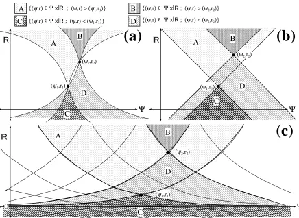
Figure 1: Upper and lower contour sets for the wicus on Ψ×Rfrom Example 2.1. Here, for visualization purposes, we suppose that Ψ⊆R, with the Euclidean metric. (a) The wicu from Example 2.1(a), with
γ= 1/2. The contour sets are bounded by curves of the formy=±p|x|. (b) The wicu from Example 2.1(a), with γ = 1. The contour sets are bounded by lines. Note that we must have γ ≤1 so that, if (ψ1, r1)(ψ2, r2), then the upper contour set of (ψ2, r2) is contained in the upper contour set of (ψ1, r1)
(as required by transitivity). (c) The wicu from Example 2.1(b). The contour sets are bounded by exponential curves of the formy=c±x.
in happiness’ for ψ as the change from (ψ′, r
1) to (ψ′, r2) represents for ψ′). However,
suppose the ‘zeros’ of different people’s utility functions are set at different locations (so (ψ,0) is not necessarily equivalent to (ψ′,0)). The precise deviation between utility zeros
of two individuals is unknown, but it is bounded by psychological distance between them. Formally, letc >0 and γ ∈(0,1) be constants. For any (ψ1, r1),(ψ2, r2)∈Ψ×R, stipulate
that (ψ1, r1)≺(ψ2, r2) iffr1+c·d(ψ1, ψ2)γ < r2, while (ψ1, r1)≈(ψ2, r2) iff (ψ1, r1) = (ψ2, r2).
See Figure 1(a,b).
(b) Suppose all individuals have cardinal utility functions with the same zero point (so for allψ, ψ′, the point (ψ,0) is equivalent to (ψ′,0) —perhaps being the utility of some ‘neutral’
be a constant. For any (ψ1, r1),(ψ2, r2)∈Ψ×R, stipulate that (ψ1, r1)≺(ψ2, r2) if either
r1 ≥0 andcd(ψ1,ψ2)·r1 < r2; or r1 <0 andc−d(ψ1,ψ2)·r1 < r2. Meanwhile, (ψ1, r1)≈(ψ2, r2)
iff either (ψ1, r1) = (ψ2, r2) or r1 = 0 =r2. See Figure 1(c). ♦
Now let Φ be any space of physical states, and for each ψ ∈ Ψ, let uψ : Φ−→R be a
utility function representing the preference order (
ψ) on Φ. Let (∗) be a wicu on Ψ×R;
then we can define awicu-mediated wipo () on Ψ×Φ by:
(ψ1, φ1)(ψ2, φ2)
⇐⇒ (φ1, uψ1(φ1))∗(φ2, uψ2(φ2))
. (3)
2.2
Hedometers
Suppose there was a scientific instrument which, when applied to any person, could ob-jectively measure her current happiness or well-being in some standard units. Call this hypothetical instrument ahedometer, and represent it as a functionh: Ψ×Φ−→R. Thus, ifh(ψ, φ)< h(ψ, φ′), then psychologyψis happier in physical stateφ′than in stateφ. Thus,
the hedometer yields an ordinal utility function representing the preference ordering (
ψ) of any fixed psychological type ψ. However, since h objectively measures utility in standard units, it can also be used to make interpersonal comparisons: if h(ψ, φ) < h(ψ′, φ′), then,
objectively, psychology ψ′ is happier in physical state φ′ than psychologyψ is in state φ.
Unfortunately, no such instrument exists, and even we had a putative hedometer in front of us, there would be no way of verifying its accuracy. However, suppose we have a collection of possible hedometers; that is, a setH of functions h: Ψ×Φ−→R such that:
• For all ψ ∈ Ψ, the function h(ψ,•) : Φ−→R is an ordinal utility function for the preference ordering (
ψ).
• For any (ψ, φ),(ψ′, φ′)∈Ψ×Φ, if (ψ′, φ′) ismuchhappier than (ψ, φ), thenh(ψ′, φ′)>
h(ψ, φ) (but not conversely).
One of the elements ofH is the ‘true’ hedometer, but we don’t know which one. Thus, we could define a wipo (
H) on Ψ×Φ as follows: for all (ψ, φ),(ψ
′, φ′)∈Ψ×Φ,
(ψ, φ)
H(ψ
′, φ′)
⇐⇒ h(ψ, φ) ≤ h(ψ′, φ′), for allh∈ H. (4)
We will see later that many wipos can be represented in this way (§4.1).
Example 2.2: (Wipo by jury) LetJ be some jury of individuals, and assume eachj ∈ J
possesses acompletewipo (
j) on Ψ×Φ, which expressesj’s own (subjective) interpersonal comparisons of well-being. The orders {
all of them must satisfy axiom (W1)). Let (
J) be the meet of the collection {j}j∈J; then Lemma 1.1(a,b) implies that (
J) is a wipo. 1
Suppose each of the complete orders (
j) can be represented by a functionhj : Ψ×Φ−→R. Then the jury’s wipo (
J) is defined by eqn.(4). ♦
In §7, we will develop more technically complicated examples of wipos, based on more detailed and plausible psychological models of interpersonal comparability. First, however, in§3-§6, we will apply wipos to make social welfare judgements.
3
Social preferences over worlds
Let I be a finite set (representing a population). A society is an element of ψ ∈ ΨI,
which assigns a ‘psychology’ ψi to each member i of the population I. A situation is an
element φ ∈ ΦI which assigns a physical state φ
i to each i ∈ I. A world is an ordered
pair (ψ,φ) ∈ ΨI ×ΦI —that is, a society together with a situation. If σ : I−→I is a
permutation, and (ψ,φ)∈ΨI ×ΦI, then define
σ(ψ,φ) := (ψ′,φ′), where ψ′
i :=ψσ(i) and φ′i :=φσ(i) for all i∈ I. (5)
Let () be a wipo on Ψ×Φ. A ()-social preference over worlds (or sprow) is a preorder (E) on ΨI×ΦI which satisfies two properties:
(ParE) For any (ψ1,φ1),(ψ2,φ2)∈ΨI×ΦI,
(ψ1
i, φ1i)(ψi2, φ2i), ∀i∈ I
=⇒ (ψ1,φ1) E (ψ2,φ2),
and (ψ1i, φ1i)≺(ψi2, φ2i), ∀i∈ I
=⇒ (ψ1,φ1) ⊳ (ψ2,φ2).
(AnonE) For all (ψ,φ) ∈ ΨI ×ΦI, if σ : I−→I is any permutation, then (ψ,φ) ≈△
σ(ψ,φ). (Here, (≈△) is the symmetric factor of (E)).
Axiom (AnonE) makes sense because the elements ofI are merely ‘placeholders’, with
no psychological content. All information about the ‘psychological identity’ of individual i is encoded in the ‘psychological state variable’ ψi. Thus, if (ψ1,φ1),(ψ2,φ2) are two
worlds, and ψi1 6=ψ2i, then it may not make any sense to compare the welfare of (ψi1, φ1i)
with (ψ2
i, φ2i) (unless such a comparison is allowed by ()), because ψ1i and ψi2 represent
different people (even though they have the same index). On the other hand, if ψ1
i =ψ2j,
1
Note that we must requireunanimous consensus in the definition of (
J); if we merely required
ma-joritarian or supermama-joritarian support [e.g. we say (ψ1, φ1)
J(ψ2, φ2) if at least 66% of all j ∈ J think
(ψ1, φ1)
j(ψ2, φ2)], then the relation (
then it makes perfect sense to compare (ψ1
i, φ1i) with (ψj2, φj2), even if i 6= j, because ψi1
and ψ2
j are in every sense the same person (even though this person has different indices
in the two worlds).
Axiom (ParE) is sometimes called ‘Weak Pareto’. We might also consider sprows which
also satisfy the following ‘Strong Pareto’ property:
(SParE
) For any (ψ1,φ1),(ψ2,φ2) ∈ ΨI ×ΦI, if (ψ1
i, φ1i)(ψi2, φ2i) for all i ∈ I, and
(ψ1
i, φ1i)≺(ψi2, φ2i) for some i∈ I, then (ψ
1
,φ1) E (ψ2,φ2).
3.1
The Suppes-Sen sprow
The Suppes-Sen sprow2 (E
s) is defined as follows: for any (ψ,φ),(ψ
′
,φ′) ∈ ΨI × ΦI,
(ψ,φ)E
s(ψ
′,φ′) if and only if there is a permutation σ : I−→I such that, for all i ∈ I,
(ψi, φi) (ψ′σ(i), φ′σ(i)). We will see shortly that (E
s) is the ‘minimal’ ()-sprow, which is extended (and often refined) by every other ()-sprow (see Proposition 3.4(b)).
Example 3.1: (Cost-benefit analysis)
Given two worlds (ψ1,φ1),(ψ2,φ2)∈ΨI×ΦI, letI
↓ :={i∈ I; (ψ1i, φ1i)≻(ψ2i, φ2i)}be the
set of ‘losers’ under the change from world (ψ1,φ1) to world (ψ2,φ2), and letI↑ :={i∈ I;
(ψi1, φ1i)≺(ψi2, φi2)}be the set of ‘winners’. LetI0 :=I \(I↓⊔I↑) be everyone else. Suppose
that:
• There is a bijectiong :I0−→I0 such that, for everyi∈ I0, (ψg1(i), φ1g(i))≈(ψi2, φ2i);
• There is an injectionh:I↓−→I↑ such that, for alli∈ I↓,
(ψ1h(i), φ1h(i)) (ψ2i, φ2i) ≺ (ψ1i, φ1i) (ψh2(i), φ2h(i)). (6)
Thus, we can pair up every ‘loser’i inI↓ with some ‘winner’ h(i) in I↑ such that the gains
for h(i) clearly outweigh the losses for i in the change from (ψ1,φ1) to (ψ2,φ2). Claim 3.1*: (ψ1,φ1)E
s(ψ
2
,φ2).
Proof. Define σ :I−→I as follows: σ(i) := g(i) for alli ∈ I0; σ(i) := h(i) for alli ∈ I↓;
σ(i) :=h−1(i) for all i∈h(I
↓)⊆ I↑; and σ(i) :=i for all other i∈ I↑\h(I↓).
It remains to show that (ψ1
i, φ1i)(ψσ2(i), φ2σ(i)) for all i∈ I. There are three cases: (1)
i∈ I0; (2) i∈ I↓ ori∈h(I↓); and (3) i∈ I↑\h(I↓).
(1): Ifi∈ I0, then (ψ1i, φi1)≈(ψg2(i), φ2g(i)) = (ψ2σ(i), φ2σ(i)) by definition of g.
(2): Ifi∈ I↓andj =h(i)∈ I↑, then (ψj1, φ1j)(ψi2, φ2i)≺(ψi1, φ1i)(ψj2, φ2j). However,
σ(i) =j and σ(j) = i; hence (ψ1i, φ1i)(ψ2σ(i), φ2σ(i)) and (ψj1, φ1j)(ψσ2(j), φ2σ(j)).
(3): If i∈ I↑\f(I↓), then σ(i) =i and (ψi1, φ1i)≺ (ψi2, φ2i); so (ψi1, φ1i)≺ (ψσ2(i), φ2σ(i)).
✸ Claim 3.1*
2
This sprow is based on thegrading principle, a partial social welfare order defined by Suppes (1966) onR2
, and extended toRn by Sen (1970b,§9*1-§9*3, pp.150-156). It was later named the ‘Suppes-Sen’
For example, suppose I = {i, j}, fix ψi, ψj ∈ Ψ, and let φ1,φ2 ∈ ΦI be two situations
such that φ1
iψiφ2i while φ2jψjφ1j. Thus, a change from situation φ
1 to φ2 would help Isolde
(i) and hurt Jack (j) —thus, neither situation is Pareto-preferred to the other. Borrowing Harsanyi’s well-known example, suppose I have an extra ticket to a Chopin concert which I can’t use, and letφ1be the situation where I give the ticket to Jack, whileφ2 is the situation where I give the ticket to Isolde. Both Isolde and Jack want the ticket. However Isolde is a classical pianist and Chopin fanatic who has been complaining bitterly for months that she couldn’t get a ticket to this sold-out concert, whereas Jack doesn’t even like classical music; he only wants the ticket because going to any concert is slightly preferable to spending a boring evening at home. Assume that, other than the concert issue, Jack and Isolde have roughly similar levels of well-being. Then we might reasonably suppose that (ψi, φ1i) (ψj, φ2j) (ψj, φ1j) (ψi, φ2i). Thus, the change from φ
1 to φ2 helps
Isolde more than it hurts Jack, so φ2 is socially preferable to φ1; hence (ψ,φ1)E
s(ψ,φ
2).
(To see this, set I↓ :={j}, I↑ :={i}, and h(j) := iin eqn.(6).) ♦
Note that we can perform the interpersonal ‘cost-benefit analysis’ in Example 3.1 with-out even a utility function, much less a complete system of IPUC. However, even if the wipo () is a complete ordering on Ψ×Φ, the sprow (E
s) is still a very partial ordering of ΨI ×ΦI. In Example 3.1, the number of ‘big winners’ in I
↑ must exceed the number
of losers (even small losers) in I↓, so that every loser can be matched up with some ‘big
winner’ whose gains outweigh her losses. Thus, (E
s) might not recognize the social value of a change φ1 ❀ φ2 where a wealthy 51% majority I↓ sacrifices a pittance so that
des-titute 49% minority I↑ can gain a fortune —something which classic utilitarianism would
recognize. In particular, it is necessary, but notsufficient, for a clear majority to support the change φ1 ❀φ2; thus, (E
s) is actually much less decisive than simple majority vote.
Example 3.2: Suppose that Φ =R, as in§2.1. Then for any (ψ1,r1),(ψ2,r2)∈ΨI×RI,
(ψ1,r1)E
s(ψ
2
,r2) if and only if there is a permutation σ : I−→I such that, for all i ∈ I,
(ψ1
i, r1i) (ψ2σ(i), r2σ(i)). Let I = {1,2} and fix ψ = (ψ1, ψ2) ∈ ΨI; then (Es) induces a preorder (◭
s,ψ) on R
2, where, for allr,r′ ∈R2, we have r′◭
s,ψr iff (ψ,r
′)E
s(ψ,r).
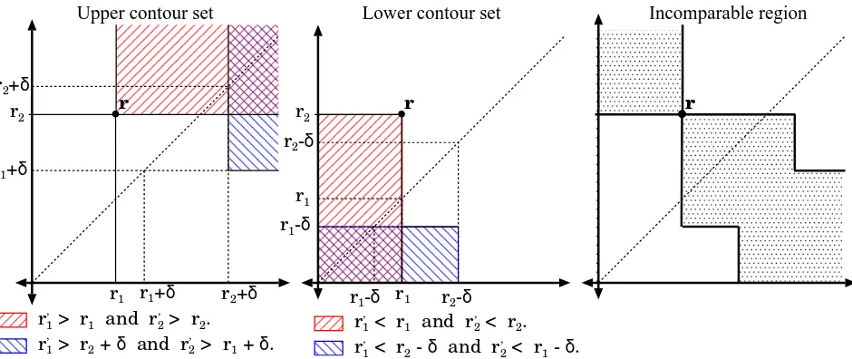
(a) Let () be the wipo on Ψ×R from Example 2.1(a), and let δ := c·d(ψ1, ψ2)γ. Fix
r∈R2. For anyr′ ∈R2, r′◭
s,ψr iff eitherr
′
1 ≤r1 andr′2 ≤r2, orr2′ ≤r1−δ and r1′ ≤r2−δ.
See Figure 2.
(b) Let () be the wipo on Ψ×R from Example 2.1(b), and let C :=cd(ψ1,ψ2). Then for any r,r′ ∈R2,r′◭
s,ψr iff either r
′
1 ≤r1 and r′2 ≤r2, or r2′ ≤r1/C and r′1 ≤r2/C. ♦
r
r1 r2
r1-δ r1-δ
r2-δ
r2-δ r1
r
r1 r2
r1+δ r1+δ
r2+δ
r2+δ
Upper contour set Lower contour set
r,1 > r2 + δ and r ,
2 > r1 + δ. r,1 > r1 and r
, 2 > r2.
r,1 < r2 - δ and r ,
2 < r1 - δ. r,1 < r1 and r,2 < r2.
Incomparable region
[image:16.595.70.540.99.297.2]r r
Figure 2: Upper and lower contour sets of the relation (◭
s,ψ) onR
2
induced by the Suppes-Sen sprow (E
s)
in Example 3.2(a). Each contour set contains two overlapping regions, corresponding to the two possible conditions implying the relationr′
◮
s,ψr(or vice versa).
The sprow of Example 3.2(b) generates similar pictures: simply replace ‘rj−δ’ with ‘rj/C’ and ‘rj+δ’
with ‘C rj’ everywhere. The difference between Examples 3.2(a) and (b) is in scaling. Using the sprow of
Example 3.2(b), if we multiplyrby a scalar, we see exactly the same pictures. However, using the sprow of 3.2(a), if we multiplyrby, say, 2, then the ‘incomparable’ region (right) will be only half as wide.
Fixψ∈Ψ2, and let (◭
s,ψ) be the preorder onR
2 from Example 3.2. An incomplete preorder
like (◭
s,ψ) may not have any weakly dominant points in B; instead, we consider the set wkUnd
B, ◭
s,ψ
of points which are weakly (◭
s,ψ)-undominated in B (see eqn.(1) in §1 for
definition). For any b ∈ B, we have b ∈ wkUndB, ◭
s,ψ
if there is no b′ ∈ B \ {b} such
thatb ◭
s,ψb
′. This means: (1) There is nob′ ∈ Bwhich Pareto-dominatesb; and (2) There
is no b′ ∈ B such thatb1 < b′2−δ and b2 < b′1−δ.
Let P′ be the reflection of P across the diagonal. Let P′′ := P − (δ, δ); then b ∈
wkUndB, ◭
s,ψ
if (1) b ∈ P and (2) There is no b′ ∈ P′′ which Pareto-dominates b.
The set wkUndB, ◭
s,ψ
is shown in Figure 3(A). ♦
Proposition 3.4 Let () be a wipo.
(a) (E
s) is a ()-sprow.
(b) If (E) is any ()-sprow, then (E) extends (E
s).
If (E) also satisfies (SParE), then (E) also refines (E
B
(C)
δ δ
P P’’ P’
B
(A)
B
P
(B)
δ δ b
1 = b 2 b1 = b
2-δ
b1 = b 2+δ
Slope =
-A
Slope =
-A
Slope =
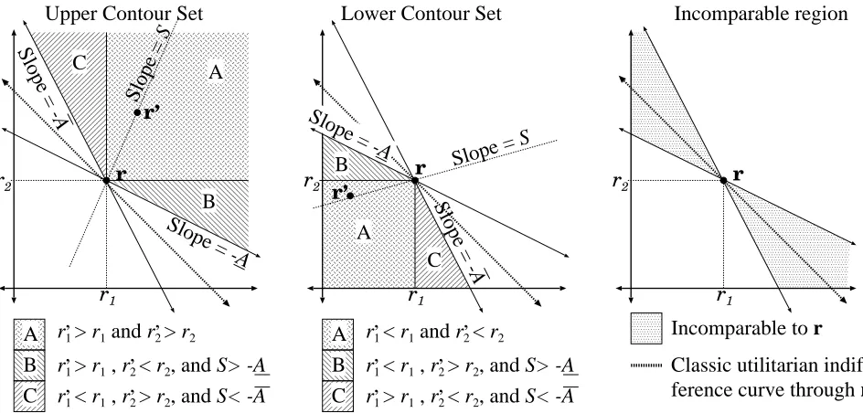
[image:17.595.79.524.110.280.2]T
Figure 3: Solving bilateral bargaining problems with sprows. (A)The Suppes-Sen bargaining solution
wkUndB, ◭
s,ψ
of Example 3.3. (B)The approximate egalitarian bargaining solutionwkUndB, ◭
æ,ψ
of
Example 3.6. (C)The approximate utilitarian bargaining solutionwkUndB, ◭
u,ψ
of Example 5.3.
(c) (Pareto Indifference) Let (E) be any ()-sprow, and let (ψ1,φ1),(ψ2,φ2) ∈
ΨI×ΦI. If (ψ1
i, φ1i)≈(ψ2i, φi2), for all i∈ I, then (ψ1,φ1)
△
≈ (ψ2,φ2).
(d) If {E
λ}λ∈Λ is a collection of ()-sprows (where Λ is some indexing set), and (E)
is their meet, then (E) is also a ()-sprow.
3.2
Approximate egalitarianism
Given a wipo () on Ψ×Φ, the ()-approximate egalitariansprow (E
æ) on Ψ
I×ΦI is defined
as follows: For any (ψ1,φ1),(ψ2,φ2)∈ΨI×ΦI,
(ψ1,φ1)E
æ(ψ
2,φ2)
⇐⇒ There is a functionsuch that, for all i∈ If :, (ψI−→I1 (possibly not injective)
f(i), φ1f(i))(ψi2, φ2i)
!
.
In other words, for every person i in the world (ψ2,φ2), no matter how badly off, we can find some personf(i) in the world (ψ1,φ1) who is even worse off. In particular, this means that even the ‘worst off’ people in (ψ2,φ2) (i.e. elements of I which are ‘minimal’ with respect to ()) are still better off than someone in (ψ1,φ1). If () is a complete ordering on Ψ×Φ, then all people in world (ψ1,φ1) are comparable with all people in (ψ2,φ2), and (E
æ) is equivalent to the classical ‘maximin’ egalitarian social welfare ordering.
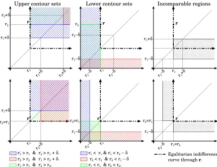
Example 3.5: Suppose that Φ =R, as in§2.1. Then for any (ψ1,r1),(ψ2
,r2)∈ΨI×RI,
(ψ1,r1)E
æ(ψ
2,r2) iff there is a functionf :I−→I (possibly not injective) such that, for all
i∈ I, (ψ1
r
r1 r2
r1+δ r1+δ
r2+δ
r2+δ
r
r1 r2−δ
Upper contour sets
r
r1 r2
r1−δ r1−δ
r2−δ
r2−δ
Lower contour sets
r
r1 r2=r1
r2+δ r1+δ
r2=r1
r1−δ
r,1 > r1 & r ,
2 > r1 + δ.
r,2 > r2 & r ,
1 > r2 + δ.
r,1 > r1 & r , 2 > r2.
r,1 < r1 & r , 1 < r2−δ
r,2 < r2 & r , 2 < r1− δ
r,1 < r1 & r , 2 < r2.
r1=r2
r2−δ r
r1
r1−δ
Incomparable regions
r2=r1
r1−δ
Egalitarian indifference curve through r. r1+δ
r1−δ r1+δ
[image:18.595.84.521.97.434.2]r
Figure 4: Contour sets for the relation (◭
æ,ψ) induced on R
2
by approximate egalitarian sprow (E
æ) in
Example 3.5. Left:the upper contour sets for two choices ofr∈R2
. Middle:the lower contour sets. Each contour set contains three overlapping regions, corresponding to the three possible conditions implying the relationr′ ◮
æ,ψr(or vice versa). Right: The incomparable regions
r′ ∈R2
; r′
◮6◭ r . For reference, we also show the indifference curve of the classical egalitarian (i.e. maximin) SWO.
Let I ={1,2} and fix ψ= (ψ1, ψ2)∈ΨI; then (Eæ) induces a preorder (æ,ψ◭) on R2, where
r′ ◭
æ,ψr iff (ψ,r
′)E
æ(ψ,r). In particular, let () be the wipo of Example 2.1(a), and let δ := c·d(ψ1, ψ2)γ. For any r,r′ ∈ R2, r′æ,ψ◭r iff either (1) r1 ≤ r1′ and r2 ≤ r′2; or (2)
r1 ≤r′1 and r1 ≤r′2−δ; or (3) r2 ≤r2′ and r2 ≤r1′ −δ. See Figure 4. ♦
Example 3.6: (Bargaining problems) Let B ⊂ R2 be some compact, convex set (e.g. a bargaining set), as in Example 3.3. Let (◭
æ,ψ) be the preorder on R
2 from Example 3.5, and
letP be the Pareto frontier ofB. Recall from Example 3.3 that the appropriate ‘bargaining solution’ in this setting is the weakly undominated set wkUndB, ◭
æ,ψ
. We have:
Claim 3.6*: wkUnd
B, ◭
æ,ψ
Given (ψ1,φ1),(ψ2,φ2) ∈ ΨI ×ΦI, let I
↓, I↑, and I0 be as in Example 3.1. We say
(ψ2,φ2) is a Hammond equity improvement over (ψ1,φ1) if
• There is a bijection g :I0−→I0 such that, for every i∈ I0, (ψg1(i), φ1g(i))≈(ψ2i, φ2i);
• There is a injection h:I↓−→I↑ such that, for all i∈ I↓,
(ψh1(i), φ1h(i)) (ψh2(i), φh2(i)) (ψi2, φi2) (ψi1, φ1i). (7)
In other words, we can pair up every ‘loser’ i in I↓ with some ‘winner’ h(i) in I↑ such
that Hammond’s (1976) equity condition is satisfied: both before and after the change, i is better off than h(i), but the change narrows the gap between them.
For example, recall the ‘concert ticket’ story from Example 3.1, but now with a different scenario. Suppose Isolde and Jack have roughly equally strong desires to attend the concert. However, Isolde is a miserable, depressed person, whereas Jack is a happy, contented person. Isolde will be less happy than Jack no matter who gets the ticket; thus, we have (ψi, φ1i) (ψi, φ2i) (ψj, φ2j) (ψj, φ1j). Thus, the change from φ
1 to φ2 reduces
inequality, so it is a Hammond equity improvement. (To see this, set I↓ :={j}, I↑ :={i},
and h(j) := i in eqn.(7).)
The next result says that the approximate egalitarian sprow (E
æ) is ‘Hammond equity promoting’.
Proposition 3.7 For any(ψ1,φ1),(ψ2,φ2)∈ΨI×ΦI, if (ψ2
,φ2) is a Hammond equity
improvement over (ψ1,φ1), then (ψ1,φ1)E
æ(ψ
2,φ2).
Proof. Let g :I0−→I0 and h:I↓−→I↑ be as in eqn.(7). Define f :I−→I as follows: For
all i ∈ I0, let f(i) :=g(i). For all i ∈ I↓, let f(i) := h(i). For all i ∈ I↑, let f(i) =i.
Then clearly, for all i∈ I, we have (ψ1
f(i), φ1f(i))(ψi2, φ2i); hence (ψ
1,φ1) E
æ(ψ
2,φ2), as
desired. ✷
4
Hedometry and Welfarism
4.1
Hedometers
LetX be a set and let () be a preorder on X. Aweak utility functionfor () is a function u:X −→R which is ‘nondecreasing’ in the following sense:
For allx, y ∈ X, xy =⇒ u(x)≤u(y). (8)
It follows that x≈y ⇒ (u(x) =u(y)). Note that (8) is a rather weak requirement —for example, any constant function is a weak utility function. A strong utility function
(or Richter-Peleg function) is a function u:X −→R which satisfies (8) and also satisfies:
Under mild hypotheses, preorders on topological spaces admit continuous strong utility functions (Richter, 1966; Peleg, 1970),3 or semicontinuous strong utility functions (Jaffray,
1975; Sondermann, 1980). Likewise, if a preorder on a space of lotteries satisfies versions of the vNM axioms of ‘Linearity’ and ‘Continuity’, then it has a linear strong utility function (Aumann, 1962).
As observed by Evren and Ok (2009), every preorder () admits a weak multiutility representation. That is, there is a setU of weak utility functions for () such that
For all x, y ∈ X, xy ⇐⇒ u(x)≤u(y), for all u∈ U. (10)
(For example: for all x ∈ X, define ux : X −→R by ux(y) := 1 if y x and ux(y) := 0 if
y6x; then it is easy to see thatU :={ux; x∈ X } is a weak multiutility representation.)
Unfortunately, such a representation will not be sufficient for our purposes, because every element of U may violate statement (9).
A strong multiutility representation for () is a set U of strong utility functions for () which satisfies statement (10). Preorders admit such representations under fairly mild hypotheses. For example, suppose () is separable, meaning there is a countable subset
Y ⊆ X which isdense(i.e. for allx≺z ∈ X, there exists somey∈ Y such thatx≺y ≺z); then () has a strong multiutility representation (Mandler, 2006, Thm.1). Furthermore, if
X is a locally compact separable metric space and () is a continuous preorder, then () admits a strong multiutility representation comprised entirely of continuous strong utility functions (Evren and Ok, 2009, Corollary 1).4
Now let () be a wipo on Ψ×Φ. Motivated by the scenario of §2.2, we will refer to a strong utility function for () as a hedometer. That is, a hedometer for () is a func-tion h: Ψ×Φ−→R such that, for all (ψ1, φ1),(ψ2, φ2)∈Ψ×Φ,
(ψ1, φ1)(ψ2, φ2)
=⇒
h(ψ1, φ1)≤h(ψ2, φ2)
and(ψ1, φ1)≺(ψ2, φ2)
=⇒h(ψ1, φ1)< h(ψ2, φ2)
. LetHED()
be the set of hedometers for (). We say that () ishedometricif it has a strong multiu-tility representation (10), with U =HED(). The aforementioned results imply that wipos
are hedometric under broad hypotheses, and that HED() itself is nonempty under even
broader hypotheses.
3
See also Levin (1983a,b, 1984, 2000), Mehta (1986), Herden (1989a,b,c, 1995), and the monographs by Nachbin (1965) and Bridges and Mehta (1995).
4
Mandler’s (2006) result is formulated in terms ofweakmultiutility representations, but an examination of the proof reveals that it actually establishes a strong multiutility representation. Ok (2002) and Evren and Ok (2009) have also constructed strong multiutility representations for topological preorders using
semicontinuous utility functions, as well as sufficient conditions for the set U in (10) to be finite; see also Yılmaz (2008). Evren and Ok (2009) have also established the existence of (semi)continuous weak
multiutility representations for topological preorders. Much earlier, Dushnik and Miller (1941) showed that any irreflexive partial order was the intersection of all its linear extensions; this result was extended to preorders by Donaldson and Weymark (1998), and to a very broad class of binary relations by Duggan (1999). However, the linear extensions involved in these intersections cannot generally be represented by utility functions. Finally, Stecher (2008, Thm.2) provides conditions under which a strict partial order (≺) onX can be represented by an ‘interval-valued’ utility function. This means there is a collectionU of
4.2
Welfarism
A social welfare order (SWO) is a complete preorder (◭) on RI satisfying two axioms:
(Par◭) For any r,r′ ∈RI, if r
i ≤ r′i for alli ∈ I, then r◭r′. If ri < r′i for alli ∈ I, then
r◭r′.
(Anon◭) Ifσ :I−→I is any permutation, andr∈RI, thenr ≈N σ(r).
Example 4.1: (a) The egalitarian SWO (◭
e) is defined as follows. For all r
1,r2 ∈ RI,
r1◭
er
2 if and only if min
i∈I (r
1
i) ≤ min i∈I (r
2
i). (Thus, r1
N
≈
e r
2 whenever min
i∈I (r
1
i) = min i∈I (r
2
i).)
(b) Suppose I := [1...I]. Let րRI := r∈RI ; r1 ≤r2 ≤ · · · ≤rI . For any r ∈ RI, let
ր
r ∈ րRI be the element obtained by arranging the entries of r in ascending order —e.g.
ր
r1 := mini∈Iri and
ր
rI := maxi∈Iri. For any k ∈[1...I], the rank k dictatorship SWO (◭
k) is defined on RI byr◭
kr
′ iff ր
rk ≤
ր
r′
k (thus, (◭e) is the rank 1 dictatorship).
(c) Thelexmin SWO (◭
lex) is defined as follows: r
1◭
lexr
2 iff there exists some j ∈[1...I] such
that րrk =
ր
r′
k for all k ∈[1...j), while
ր
rj <
ր
r′
j. Meanwhile, r1
N
≈
lex r
2 iff r1 =r2. ♦
For any (ψ,φ) ∈ ΨI × ΦI and function h : Ψ × Φ−→R, we define h(ψ,φ) :=
(h(ψi, φi))i∈I ∈RI.
Proposition 4.2 Let () be a wipo on Ψ×Φ. Let (◭) be a complete preorder on RI
satisfying axiom (Par◭
), and let h: Ψ×Φ−→R be some function. Define the preorder (E
h)
on ΨI×ΦI by (ψ,φ)E
h(ψ
′
,φ′) iff h(ψ,φ)◭h(ψ′,φ′). Then
E
h is a ()-sprow
⇐⇒ h∈ HED() and (◭) is a SWO
.
Corollary 4.3 Let () be a wipo on Ψ×Φ, and let H ⊆ HED() be some collection of
hedometers. Let (◭) be a SWO on RI, and define the preorder (E
H) on Ψ
I ×ΦI by
(ψ,φ)E
H(ψ
′,φ′)
⇐⇒ h(ψ,φ) ◭ h(ψ′,φ′), for allh∈ H.
Then (E
H) is a ()-sprow.
Proof. Combine Proposition 4.2 with Lemma 3.4(d). ✷
The set HED() generally contains many possible hedometers, which could yield
Thus, for any SWO (◭) onRI, the (,◭)-welfarist5 sprow (E) is defined as follows: for all (ψ1,φ1),(ψ2,φ2)∈ΨI ×ΦI,
(ψ1,φ1)E(ψ2,φ2) ⇐⇒ For all h∈ HED(), h(ψ1,φ1)◭h(ψ2,φ2)
. (11)
The welfarist sprow (11) seems most plausible when () is hedometric, but it is well-defined whenever HED()6=∅.
Proposition 4.4 Let () be a hedometric wipo. Let (◭
e) be the egalitarian SWO in
Ex-ample 4.1(a). The (,◭
e)-welfarist sprow is the approximate egalitarian sprow (Eæ) from
§3.2. In other words, for any (ψ1,φ1),(ψ2,φ2)∈ΨI×ΦI,
(ψ1,φ1)E
æ(ψ
2
,φ2) ⇐⇒ mini∈I h(ψ1i, φ1i)≤min i∈I h(ψ
2
i, φ2i), ∀ h∈ HED()
.
In general, a ()-sprow will be a very incomplete preorder on ΨI ×ΦI, because ()
itself is an incomplete preorder of Ψ×Φ. Say that two worlds (ψ,φ),(ψ′,φ′)∈ΨI ×ΦI
are fully ()-comparable if the set {(ψi, φi)}i∈I ∪ {(ψi′, φ′i)}i∈I is totally ordered by ().
(For example, fix ψ ∈ Ψ, and suppose (ψ,φ) and (ψ′,φ′) are ‘ψ-clone worlds’ where ψi =ψ′i =ψ for alli∈ I; then (ψ,φ) and (ψ
′,φ′) are fully ()-comparable). In this case,
a ()-sprow really has no excuse for failing to order (ψ,φ) relative to (ψ′,φ′), since every element of {(ψi, φi)}i∈I is ()-comparable to every element of {(ψi′, φ′i)}i∈I. A ()-sprow
(E) isminimally decisiveif (ψ,φ) and (ψ′,φ′) are (E)-comparable whenever they are fully ()-comparable.
Example 4.5: The approximate egalitarian sprow (E
æ) (see §3.2) is minimally decisive. To see this, suppose (ψ1,φ1) and (ψ2,φ2) are fully ()-comparable. Then there exists some m ∈ {1,2} and some j ∈ I such that (ψm
j , φmj )(ψin, φni) for all (n, i) ∈ {1,2} × I.
Supposem= 1, and definef :I−→I byf(i) = j for alli∈ I; then we have (ψ1
f(i), φ1f(i)) =
(ψ1
j, φ1j)(ψi2, φ2i) for all i∈ I; hence (ψ
1
,φ1)E
æ(ψ
2
,φ2). ♦
We will now show that very few welfarist sprows are minimally decisive, and among these, only the approximate egalitarian sprow has a desirable ‘equity’ property. To explain this, suppose (ψ1,φ1),(ψ2,φ2) ∈ ΨI ×ΦI are fully ()-comparable. The rank structure
of the pair ((ψ1,φ1),(ψ2,φ2)) is the complete order (⋖) on {1,2} × I defined as follows: for all n, m ∈ {1,2} and i, j ∈ I, (n, i)⋖(m, j) if and only if (ψn
i, φni)(ψjm, φmj ). We will
require the following axiom of ‘minimal richness’ for ():
5
(MR) For any complete order (⋖) on{1,2}×I, there exist fully ()-comparable (ψ1,φ1) and (ψ2,φ2) in ΨI×ΦI whose rank structure is (⋖).
This is a very mild condition, which is satisfied by almost any collection of preferences. For example, suppose there exists some subset Φ′ ⊆Φ with|Φ′| ≥2× |I|, and someψ ∈Ψ
such that (
ψ) is a strict ordering of Φ
′; then () satisfies (MR). (Let ψand ψ′ be ‘ψ-clone
societies’ with ψi =ψi′ =ψ for all i ∈ I; then pick {φi}i∈I and {φ′i}i∈I from Φ′ to obtain
any desired rank structure).
We will use the following ‘minimal’ version of Hammond’s equity condition:
(MinEqE) There exist (ψ,φ),(ψ′,φ′)∈ΨI×ΦI and i, j ∈ I such that:
(q1E) (ψ
i, φi)≺(ψi′, φ′i)(ψ′j, φ′j)≺(ψj, φj).
(q2E
) (ψi, φi)(ψk, φk)≈(ψk′, φ′k) for allk ∈ I \ {i, j}; and
(q3E) (ψ,φ)E(ψ′,φ′).
We now come to the main result of this section.
Theorem 4.6 Let () be a wipo on Ψ×Φ which satisfies (MR), with HED() 6= ∅. Let
(◭) be a SWO on RI, and let (E) be the (,◭)-welfarist sprow on ΨI×ΦI.
(a) (E) is minimally decisive if and only if (◭) refines a rank dictatorship SWO
[Example 4.1(b)].
(b) If (E) is minimally decisive and satisfies (MinEq), then (E) is extended by the
approximate egalitarian sprow (E
æ).
(c) If (E) refines (E
æ), then (E) is minimally decisive and satisfies (MinEq).
(d) (E) extends (E
æ) if and only if (E) is (Eæ).
Example 4.7: Let (◭
lex) be the lexmin SWO [Example 4.1(c)], and let (
E
lex) be the (,
◭
lex )-welfarist sprow. Then (E
lex) is minimally decisive (by Lemma 4.9 in the Appendix) and satisfies (MinEq). If (ψ1,φ1)E
lex(ψ
2,φ2), then h(ψ1,φ1)◭
lexh(ψ
2,φ2) for all h ∈ H ED();
hence h(ψ1,φ1)◭
æh(ψ
2,φ2) for all h ∈ H
ED(), so (ψ1,φ1)E
æ(ψ
2,φ2). Thus, (E
æ) extends (E
lex). ♦
Let W() be the set of all welfarist sprows for the wipo (), and consider the partial order relation “⊆” on W() (i.e. (E
1) ⊆ (
E
2) iff (
E
2) extends (
E
1)). If () is hedometric then Proposition 4.4 says that (E
æ) ∈ W(). In this case, Theorem 4.6(d) says that (Eæ) is a local (⊆)-maximum in W(), while Theorem 4.6(b) says that (E
However, Theorem 4.6 applies even when () is not hedometric (so (E
æ) itself might not be inW()).
Let X ⊂ ΨI × ΦI be some set of ‘feasible’ worlds, and suppose the social planner
wishes to find the (E)-optimal world in X. If (E) is welfarist, minimally decisive, and minimally equitable, then Lemma 1.1(g)[i] and Theorem 4.6(b) imply thatwkDom(X,E)⊆
wkDomX,E
æ
and strUndX,E
æ
⊆ strUnd(X,E). In particular, if there is a unique weakly (E
æ)-dominant feasible world (ψ,φ) in X, then (ψ,φ) is the only possible weakly (E)-dominant feasible world in X. On the other hand, any strictly (E
æ)-undominated feasible world is also strictly (E)-undominated.
Suppose further that X is small enough that (E) is a complete ordering when re-stricted to X. Then (E
æ) is also complete onX (by Lemma 1.1(c)), and hence (E) refines (E
æ) (by Lemma 1.1(d)). Thus, Lemma 1.1(g)[ii] says
strDomX,E
æ
⊆ strDom(X,E) ⊆
wkUnd(X,E) ⊆ wkUndX,E æ
. In particular, any bargaining solution proposed by (E) must be asubset of the approximate egalitarian bargaining solution described in Example 3.6 and portrayed in Figure 3(b).
Remark. Define a ‘weak hedometer’ to be any weak utility function for () [i.e. a function u: Ψ×Φ−→Rwhich satisfies statement (8) but not necessarily (9)]. Then every
wipo is ‘weakly hedometric’, in the sense that statement (10) is always true when we take
U to be the set of all weak hedometers. Thus, if we defined a ‘weakly welfarist sprow’ by replacing HED() with the set of all weak hedometers in defining formulae (11), then we
would have a concept applicable to any wipo. However, Proposition 4.2 warns that the resulting social order may not always be a sprow. Proposition 4.4 is still true (the proof does not use (9)]. However, the proof of Theorem 4.6 breaks down if (9) is violated.
5
Weak interpersonal comparisons of lotteries
The theory of wipos and sprows developed in sections 2-4 cannot model decision-making under uncertainty. We now remedy this. LetP(Φ) be the space of probability distributions over Φ (with respect to some sigma algebra on Φ). For all ψ ∈Ψ, let (
ψ) be a complete preorder on P(Φ) which satisfies the von Neumann-Morgenstern (‘vNM’) axioms. (Thus, (
ψ) could be represented as maximizing the expected value of a cardinal utility function). Let P(Ψ) be the space of probability distributions over Ψ (with respect to some sigma algebra on Ψ), and let P(Ψ×Φ) be the space of lotteries—that is, probability measures on the product sigma algebra on Ψ×Φ. For anyδ ∈P(Ψ) andρ∈P(Φ), let δ⊗ρ∈P(Ψ×Φ) denote the unique lottery over Ψ×Φ such that (δ⊗ρ)(Ψ′ ×Φ′) = δ(Ψ′)·ρ(Φ′) for all
measurable subsets Ψ′ ⊆Ψ and Φ′ ⊆Φ.