PLACEMENT AND SIZING OF DISTRIBUTED GENERATORS IN DISTRIBUTED NETWORK BASED ON LRIC AND LOAD GROWTH CONTROL

© 2005 - 2013 JATIT & LLS. All rights reserved.

ISSN: 1992-8645 www.jatit.org E-ISSN: 1817-3195

10

STATIC ANALYSIS OF WAVELENGTH TUNING IN TWO

SECTION INDEX COUPLED DFB LASERS USING THE

TRANSFER MATRIX METHOD

1_H.BOUSSETA, 2_A.ZATNI, 3_A.AMGHAR, 4_A.MOUMEN, 5_A.ELYAMANI

1,4,5

PhD Student, M.S.I.T Laboratory, Department of Computer Engineering, high school of technology,

Ibn Zohr University, Agadir Morocco.

2_{Prof., Department of Computer Engineering, high school of technology, Agadir Morocco}

3_{Prof., Department of physics, faculty of sciences, Ibn Zohr university, Agadir Morocco}

E-mail: 1 [email protected]

ABSTRACT

The wavelength tuning is an important issue for distributed feedback (DFB) lasers designs and applications. In this paper we have presented an algorithm to analyze the wavelength tuning characteristics of two-section index-coupled (TS-IC) DFB lasers in above threshold regime, by the means of the transfer matrix method (TMM), and the carrier rate equation. The versatility of the theoretical model in the present work is demonstrated in an analysis of static characteristics of TS-IC-DFB lasers, which illustrated the important influence of coupling coefficient, cavity condition and injection current on the wavelength tuning. Therefore, The TS-IC-DFB lasers will be useful in optical communication systems using wavelength division multiplexed (WDM) networks.

Keywords:Wavelength Tuning, Distributed Feedback (DFB) Lasers, Transfers Matrix Method (TMM),

Static Characteristics.

1. INTRODUCTION

Wavelength-division-multiplexing (WDM) network need key component with high quality such as highly stable and high output power laser light source [1-2]. The distributed feedback DFB semiconductor laser is one of the fine light sources and has been widely used in optical fiber communication systems, and this is because of their small size, low power consumption, high-speed modulation capability, ultra low threshold current and possible integration with other optical functional devices [3-6].

In Optical communication systems, the static characteristics of DFB semiconductor laser such photon density, carrier density and refractive index [5-7] are important parameters that should be properly predicted. Thereby, to simulated the static effects in the semiconductor DFB lasers, It is common to use a transfer-matrix-method (TMM) [8-9] based on the counter propagation coupled mode equations [8-10], in addition to the carrier rate equation [11].TMM was first proposed by BJORK and NILSSON [12] and the first team

using it for analyzing the transmission and reflection gains in the laser amplifiers with corrugated structures was YAMADA and SUMATSN [11].

The tunable semiconductor lasers like DBR lasers [8] [13] [14] [15], DFB laser and other types of lasers had relatively simple tuning Mechanisms, and have been fully theoretically analyzed [8] [16], thus some papers also discussed the wavelength tuning proprieties of multi-electrodes DFB [17]. However the DFB laser cannot achieve as good tuning as DBR lasers, but DFB types do not give a large line-width or rather FM noise and probably also did not gave high speed[18-22].

11 the model and theory of analysis in the frame of TMM. Section 3: we study the wavelength tuning characteristics, taking into account the impact of technical and geometric parameters of the TS-IC-DFB laser such as coupling coefficient, facet reflectivity, current injection and the cavity length. Section 4: comprises the conclusion of this paper.

2. TRANSFER MATRIX METHOD FOR

TWO-SECTION INDEX COUPLED DFB LASERS

The two section index-coupled DFB laser investigated in this work is depicted schematically in fig.1. It is consists of two sections, section A and section B, with independent injection. The first section (section A) extends from z=0 to z=L/2, the second section (section B) from z=L/2 to z=L.

Fig.1. Schematic Diagram Of A TS-IC-DFB Laser

The basis of the transfer matrix method is to divide the laser longitudinally into a

number of sections, and in each section the structural and material parameters are assumed to be homogenous.

Each section is then described by a 2 by 2 complex transfer matrix, which represents the relation between forward and backward propagation waves. The transfer matrix of the corrugated section between zi+1 and zi can be

pressed by [11].

11 12

1

21 22

( ) t ( )

(

/

)

( ) t ( )

i i

t

z

z

T z

z

t

z

z

+





= 







(1)

Where

z

_i

i

L

i z

M

=

= ∆

.

L

is the length of the

cavity and M is the total number of sub-sections.

In each sub-section all parameters are assumed constant. So, the forward and the backward propagating waves in each sub-section are related to the next sub-section by the matrix

1

1 1

(

)

(

)

(

/

)

(

)

(

)

i i

i i

i i

R z

R z

T z

z

S z

S z

+

+ +









=

















(2)

( )

R z

and

S z

( )

are the slowly-varying amplitudes of forward and backward propagating fields, and the elements of transfer matrix are given by :

(

2

)

11

(

)

2

1

o

j z j

i

E

E

t

z

ρ

e

β

e

ρ

+ −

− Ω

−

=

−

(3)

(

)

12

(

)

2

1

o

j z j

i

E

E

t

z

ρ

e

β

e

ρ

+ −

− − Ω

−

−

=

−

(4)

(

)

21

(

)

2

1

o

j z j

i

E

E

t

z

ρ

e

β

e

ρ

+ −

Ω

−

=

−

(5)

(

2

)

22

(

)

2

1

o

j z j

i

E

E

t

z

ρ

e

β

e

ρ

+ −

− Ω

−

−

=

−

(6)

Where

β

₀ is the propagation constant, given by:

0

π

β

_{= Λ}

(7)

And

₍

₎

(zi1 zi)

i

E

±

z

=

e

±γ +− ₍₈₎

Λ

is the grating period of the DFB laser,

Ω

is the phase discontinuity between section i+1 and i, and

ρ

is given as:

(

)

(

)

(

)

(

)

i

i i i

jk

z

z

j

z

z

ρ

α

δ

γ

=

−

+

(9)

Where

γ

is the complex propagation, given by:

(

)

2 ₂

(

z

_i

)

(

z

_i

)

j

(

z

_i

)

k

γ

=

α

−

δ

+

(10)

With

α

and

δ

are respectively, the gain and detuning for the propagation modes taking the left section as a reference,

k

is the complex coupling constant.

For TS-IC-DFB laser had a uniform cavity, one must determine both the amplitude gain coefficient

α

, and the detuning coefficient

δ

for the section i in order that each matrix elements

( ,

1, 2)

jm

t

=

j m

=

as shown in equations (3)-(4)-(5) and (6) can be determined. For a grating with a rA

0 Section A L/2 Section B L rB

R

S

IA IB

© 2005 - 2013 JATIT & LLS. All rights reserved.

ISSN: 1992-8645 www.jatit.org E-ISSN: 1817-3195

12 first-order bragg diffraction, the mode detuning and the gain can be expressed respectively for an arbitrary section i by [11]:

2

2

(

_i

)

(

_i

)

g

(

_B

)

B

n

z

π

n z

π

π

δ

λ λ

λ

λλ

=

−

−

−

Λ

(11)

And

(

)

(

)

2

i s

i

g z

z

α

α

=

Γ

−

(12)

Where

λ

is the lasing mode wavelength,

λ

_B is the bragg wavelength,

n

_g is the group refractive

index,

n

is the refractive index,

α

_s is the constant cavity loss,

Γ

is the optical confinement factor, and the material gain

g

for semiconductors is expressed as[7]:

2

0 0 1 0 2 0

( )

_i

( ( )

_i

)

[

(

( ( )

_i

))] (13)

g z

=

A N z

−

N

−

A

λ λ

− −

A N z

−

N

With

A

₀is the differential gain,

N

is the carrier

concentration,

N

₀is the carrier density at

transparency,

λ

₀is the peak wavelength at transparency,

A

₁and

A

₂and are parameters used

in the parabolic model assumed for the material gain.

The effective refractive index can be expressed as [7]:

(

_i

)

_o

dn

(

_i

)

n z

n

N z

dN

=

+ Γ

(14)

Where

n

₀ is the refractive index and

dn

dN

is

the differential index.

On the other hand, the average carrier density in the active region along the laser cavity is described by the carrier rate equation as [11]

,

(

)

(

)

A B

i st i

I

R z

R

z

qV

=

+

(15)

With

2 3

(

)

(

)

i

(

)

(

)

i i i

N z

R z

BN

z

CN

z

τ

=

+

+

(16)

( ) ( )

( )

1

( )

g i i

st i

i

C g z P z

R

z

P z

ε

=

+

(17)

Where

I

_{A B,} is the uniform current bias of section

denoted by the subscript.

q

is the electron charge,

V

is the cavity volume, the parameter

τ

stands for the electron lifetime,

B

and

C

are bimolecular and auger recombination coefficient respectively,

g g

C

=

c n

is the group velocity, with

c

is the speed of light in vacuum, and

ε

is a non-linear coefficient to take into account saturation effects.

The photon density

p z

(

_i

)

is given by [11]

2 2

2 0

2

( )

( )

_i o

n z n

i g

( )

_i

( )

_i

(18)

P z

c

R z

S z

hc

ε

λ

_

_

=

_

+

_

Where

ε

_ois the free space permittivity,

h

is the Planck’s constant and

c

₀ a dimensionless

coefficient that allows the determination of the total electric field at the above-threshold regime, taking into account that the normalization

2 2

(0)

(0)

1

R

+

S

=

(19)

From the threshold studies [7] [11], the threshold

carrier concentration

N

_thcan be obtained from

equations (11) – (12), and such that

0

(

2

) /

0

th s th

N

=

N

+

α

+

α

Γ

A

(20)

At threshold conditions, we assumed that the

1 2

0

A

=

A

=

and

δ δ

=

_th, consequently from equation (10), we can express the threshed refractive index and the threshold wavelength such that [11]:

0

th th

n

n

n

N

N

∂

=

+ Γ

∂

(21)

2

(

)

2

/

B g th

th

th B g B

n

n

n

πλ

λ

δ λ

π

λ π

+

=

+

+

Λ

(22)

The boundary conditions are described by:

(0)

j BL

(0)

A

R

=

r e

− β

S

(23)

( )

j BL

( )

B

R L

=

r e

− β

S L

(24)

Where

r

_Aand

r

_B are the facet reflectivity of

13

3. SIMULATIONS RESULTS AND

DISCUSSIONS

[image:4.612.98.519.33.644.2]

In this paper, the numerical procedure for the above-threshold calculations follows closely the algorithm developed in [11], it is used only for a DFB laser with a single electrode, but in our work we have been developing it for the case of a DFB laser with two electrodes. The algorithm was implemented using the programming language C+ +. A flowchart of the numerical algorithm can be explained by Fig.2, which illustrates how all the various mechanisms are related to one another, each step of this flowchart is a sub program elementary with its own algorithm.

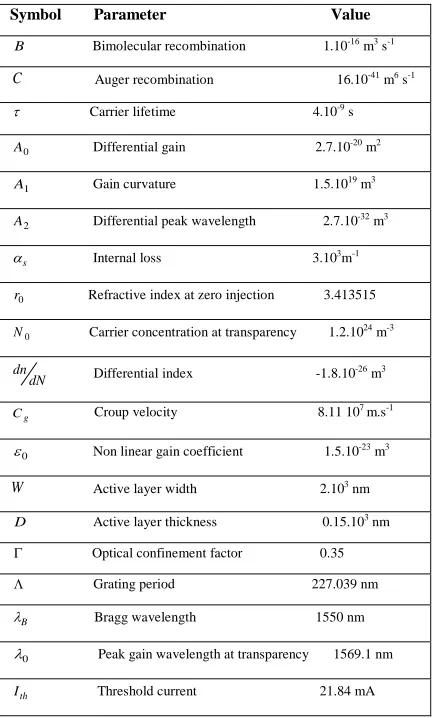
Table 1: Parameters Values Used In Simulations.

Symbol Parameter Value

B Bimolecular recombination 1.10-16 _m3 _s-1

C Auger recombination 16.10-41 _m6 _s-1

τ Carrier lifetime 4.10-9 _s

0

A Differential gain 2.7.10-20 _m2

1

A Gain curvature 1.5.1019 _m3

2

A Differential peak wavelength 2.7.10-32 _m3

s

α Internal loss 3.103_m-1

0

r Refractive index at zero injection 3.413515

0

N Carrier concentration at transparency 1.2.1024 _m-3

dn

dN Differential index -1.8.10 -26 _m3

g

C Croup velocity 8.11 107 _m.s-1

0

ε Non linear gain coefficient 1.5.10-23 _m3

W Active layer width 2.103 _nm

D Active layer thickness 0.15.103 _nm Γ Optical confinement factor 0.35

Λ Grating period 227.039 nm

B

λ Bragg wavelength 1550 nm

0

λ Peak gain wavelength at transparency 1569.1 nm

th

I Threshold current 21.84 mA

With the modeling described in second section, the static tuning characteristics of TS-IC-DFB laser were simulated and demonstrated with the parameters given in table1.

Fig.2. Flowchart Of Static Numerical Algorithm. We evaluated the longitudinal distribution of the carriers and photons along the cavity by dividing the cavity length into sub-sections of equal length. In our simulations a large number of transfer matrices must be used for a 300μm long DFB laser, at least 300 transfer matrices have been adapted to

(αL,δL th)

Calculate

Nth , Ith,λth ,nth

For IB=Ith to IB=4Ith

New formation (C0, )λ grid

[ 0 ] [ 0 ] 0

R =S =

[ 1] _{( /)} [ ] 1 [ 1] [ ]

R i _{T z z} R i i i S i S i

+

 = +  

 +  

   

[ ] 0 n [ ]

n i n N i

N ∂ = +

∂

2 3

[ ] [ ]

,

[ ] [ ] ₁

IA B N i g i P

BN i CN i C eV = τ + + + g +εP

2 2 2

[ ] o gn [ ] [ ] [ ]

P i _hc n i CoR i S i

ε λ _{ }

= _ + _

 

Solving equation using the Newton-Raphson technique

( [ ], [ ], [ ], , ,0) 0

f R i S i N i Iλc =

verification of boundary conditions

repeat the calculations with (c0, )λfinal

Output results

1 8

IB= +IB Ith

End simulation Store N i[ ] P i[ ] ,n i[ ] ,g i[ ] Solving equation j Lγ =±kLsin(γL) using the

Newton-Raphson technique

No

[image:4.612.85.301.275.634.2]

© 2005 - 2013 JATIT & LLS. All rights reserved.

ISSN: 1992-8645 www.jatit.org E-ISSN: 1817-3195

14 evaluate the static characteristics of our device. For demonstration of the tuning mechanism, when the currents are pumping asymmetry, it is interesting to see under different bias conditions the evolution of photon density, carrier density and refractive index in the cavity. All results are shown in Fig.3.

0 50 100 150 200 250 300

0 1 2 3 4 5 6 7 8

*1021

IA=1.7Ith, IB=3,3Ith

I

A=1.5Ith, IB=3,1Ith

IA=1.9Ith, IB=1.9Ith

IA=1.9Ith, IB=3,1Ith

phot

on de

ns

it

y

P

(z

) (

m

-3

)

Z in µm

(a)

0 50 100 150 200 250 300

2,0 2,2 2,4 2,6 2,8 3,0 3,2 3,4 3,6 3,8

C

ar

ri

er

d

en

si

ty N

(z

) (

m

-3)

Z in µm

IA=1.9Ith, IB=1.9Ith

IA=1.5Ith, IB=3.1Ith

IA=1.7Ith, IB=3.3Ith

IA=1.9Ith, IB=3.1Ith

*1024

(b)

0 50 100 150 200 250 300

3,390 3,391 3,392 3,393 3,394 3,395 3,396 3,397 3,398 3,399 3,400 3,401

R

ef

ract

ive i

n

d

ex n

(z

)

Z in µm

I_A=1.7I_th,I_B=3.3I_th I_A=1.5I_th, I_B=3.1I_th I_A=1.9I_th, I_B=3.1I_th I_A=1.9I_th, I_B=1.9I_th

(c)

Fig.3. Longitudinal Distribution Of (A) Photon Density, (B) Carrier Density, (C) Refractive Index In TS-IC-DFB Lasers For Different Biasing Currents, With L=300μm

And Kl=2.

The photon localization is controllable by changing the current injection ratio between different sections, this may cause a wavelength shift. Thereby, when the current increase, the longitudinal of the photon density and carrier

density also increase for all pairs of current, Fig .3.a and b, respectively shows photon density and the carrier concentration profiles. On the other hand the variations of the spatially distributed refractive index are illustrated in Fig.3.c. We observe that the refractive index decreases when the current also increases, i.e. when the photon density increases. All measurement of Fig.3, were conducted with a geometry of L=300μm and kL=2. In order to provide a deeper understanding the wavelength tuning characteristics, we present the effects of coupling coefficient, cavity condition and injections currents on the wavelength tuning.

The wavelength tuning characteristics are shown in fig.4, with IA=1.7Ith (a), IA=1.9Ith (b),

IA=2.5Ith (c). Therefore, we have the emission

wavelength λ(μm) as a function of the injection current in section B, where kL=2 and L= 500 μm

1,5 2,0 2,5 3,0 3,5 4,0 4,5

1545,0 1545,5 1546,0 1546,5 1547,0 1547,5

w

a

v

e

le

ngt

h (

nm

)

IB/Ith

IA=1.7 Ith

(a)

1,5 2,0 2,5 3,0 3,5 4,0 4,5 5,0 1544,90

1545,25 1545,60 1545,95 1546,30 1546,65

w

a

v

e

le

ngt

h (

nm

)

IB/Ith

IA=1.9 Ith

15

2,0 2,5 3,0 3,5 4,0 4,5 5,0 5,5 6,0

1545,60 1545,95 1546,30 1546,65 1547,00 1547,35

w

a

v

e

le

ngt

h (

nm

)

IB/Ith

IA=2.5 Ith

(c)

Fig.4. Wavelength Tuning Characteristics Of TS-IC-DFB Lasers For Different Biasing Currents Of Section A, (A) IA=1.7Ith, (B) IA=1.9Ith, (C) IA=2.5Ith , With L=500Μm

And Kl=2.

Whenthe injection current in the section A as IA=1.7Ith , we observe that the emission wavelength

varies discontinuously. We get 8 continuous tuning ranges with a maximum tuning range of 0.41nm. These ranges are separated by mode hopping. However, when the injection current in the first section as IB=1.9Ith or IB=2.5Ith .in this case, a

clear reduction of the tuning range is obtained ,we get only 7 continuous tuning ranges, with a maximum tuning range of 1nm. This is caused by the low injected carrier density in the cavity. We can say that the wavelength is electronically tuned by the currents.

The Fig.5 Shows the wavelength tuning characteristics for different lengths of the cavity depending on the current IB, with IA=1.8Ith and

kL=2. The maximum tuning range 1.1nm, 0.7nm and 0.4nm are obtained for the cavities of lengths as L=300µm, L=400µm and L=500µm (LA=LB=L/2) respectively. For the same bias

current, its density increases when we reduce the length of the cavity, which increases the carrier density inside the cavity. This explains that for the same excursion of current, a large range of tenability is obtained with the shortest lasers.

1,5 2,0 2,5 3,0 3,5 4,0 4,5 1544,90

1545,25 1545,60 1545,95 1546,30 1546,65

w

a

v

e

le

ngt

h (

nm

)

Ith

L=500 µm L=400 µm L=300 µm

Fig.5. Wavelength Tuning Characteristics Of TS-IC-DFB Lasers For Different Lengths Of The Cavity, With

IA=1.8Ith And Kl=2.

The Fig.6 shows the evolution of the emission wavelength λ(μm) as a function of the injection current in section B, When the injection current in section A is fixed at lA= 2lth. So, the figure

compares the wavelength tuning characteristics of two lasers for two different coupling coefficients (kL=2 and kL=4) and for the same injection currant. If the coupling coefficient is kL=2, we observe that the number of the continuous tuning is decreases and the overall tuning range is extended to 0.73nm.

1,5 2,0 2,5 3,0 3,5 4,0 4,5 1545,5

1546,0 1546,5 1547,0 1547,5 1548,0

w

a

v

e

le

ngt

h (

nm

)

IB/Ith

k=2/L k=4/L

Fig.6. Wavelength Tuning Characteristics Of TS-IC-DFB Lasers For Different Values Of Coupling Coefficients,

With IA=2Ith And L=500 Μm.

Finally, to show The dependence of the wavelength tuning on facet reflectivity the device is simulated for different values of first facet reflectivity rA, with facet reflectivity rB=0, thus the

© 2005 - 2013 JATIT & LLS. All rights reserved.

ISSN: 1992-8645 www.jatit.org E-ISSN: 1817-3195

16

2,5 3,0 3,5 4,0 4,5 5,0 5,5 6,0

1545,60 1545,95 1546,30 1546,65 1547,00 1547,35

w

a

v

e

le

ngt

h (

nm

)

IB/Ith

r_a=0,3 r_a=0,2 r_a=0

Fig.7. Wavelength Tuning Characteristics Of TS-IC-DFB Lasers For Different Values Of Facet Reflectivity Of

Section A, With IA=2.5Ith, L=500 And Kl=2.

4. CONCLUSION

With a more efficient algorithm based on TMM and carrier rate equation, we have investigated the wavelength tuning characteristics of TS-IC-DFB laser. Furthermore, the longitudinal distribution of photon density, carrier density, reflective index as well as losing wavelength was presented. We have also analyzed the effects caused by changing structural parameters on wavelength tuning, a maximum tuning range of 1.1 nm in our laser has been observed .We believe that more devices can also be analyzed using TMM and will form the subject of a future study.

REFRENCES:

[1] A. Zatni, D. Khatib, M. Bour J. Le bihan, “ Analysis of the spectral stability of the three pahse shift DFB laser (3PS-DFB)”, Annals of telecommunication, vol. 59, 2004, pp.1031-1044.

[2] M. saeed Tahvili, M. Hossein Sheikhi, “steady state analysis of optical bistability in distributed coupling coefficient DFB semiconductor laser amplifiers”, Solid-state Electronics, vol.53, 2009, pp. 79-85.

[3] M.Jabbari, M.K. Moravvej Farshi, R. Ghayour, A. Zarifkar, “SPM response of a distributed coupling coefficient DFB-SOA all- optical flip-flop”, Majlesi Journal of Electrical Engineering, vol.4,No=.1, 2010, pp. 1-6.

[4] Olaf Brox, Stefan Bauer, Mindaugas Radziunas, Matthias Wolfrum Wolfrum, Tan Sieber, Jochen Kreissl, Bernd Sartorius and

hans-jurgen Wunsche, “High-frequency pulsation in DFB lasers with amplified feedback”, IEEE journal of Quantum Electronics, vol.39,No.11, 2003, pp. 1381-1387.

[5] A. Moumen, A. Zatni, A. elkaaouachi, H. Bousseta, A. Elyamani, “A novel design of quarter wave-shifted diqstributed feedback semiconductor laser for highpower single -mode operation”, JATIT Journal of theoretical and applied information technology, Vol. 38, No. 2, 2012, pp. 210-218.

[6] M.G. Davis, R.F. O’dowd, “ A transfer matrix method based large-signal dynamic model for multielectrode DFB lasers”, IEEE journal of Quantum Electronics, vol.30, 1994, pp. 2458-2466.

[7] josé A.P. Morgado, Carlos A.F. Fernandes, josé B.M. Boavida, “ novel DFB structure suitable for stable single longitudinal mode operation”,

Optics & Laser technology, vol.42, 2010, pp. 975-984.

[8] Kai Shi, Yonglin Yu, Ruikang Zhang, Wen Liu, Liam P. Baryy,”Static and dynamic analysis of side-mode suppression of widely tunable sampled grating DBR (SG-DBR) lasers”, optics communications, vol.282, 2009, pp. 81-87. [9] Drew N. Maywar, Govind P. Agrawal,

“Transfer-matrix analysis of optical bistability in DFB semiconductor laser amplifiers with nonuniform gratings”, IEEE journal of Quantum Electronics, vol.33, 1997.pp. 2029-2037.

[10] M.G. Davis, R.F. O’dowd, “A transfer matrix method based large-signal dynamic model for multielectrode DFB lasers”, IEEE journal of Quantum Electronics, vol.30, 1994, pp. 2458-2466.

[11] H. ghafouri-shiraz, distributed feedback laser diodes and optical tunable filters, Birmingham, UK : WILEY ,2003

[12] Gunnar Bjork, Olle Nilsson, IEEE J. Lightwave Techno. LT-5.1987, pp. 140-148. [13] A. Zatni, J. Le bihan, ”Analysis of FM and

AM responses of a tunable three-electrode DBR laser diode”, IEEE journal of Quantum Electronics, vol.31 ,1995, pp.1009-1014. [14] Giora Griffel, Robert J.Lang, Amnon Yariv,

17 [15] J.B. Ekanayake and N. Jenkins, “A

Three-Level Advanced Static VAR Compensator”,

IEEE Transactions on Power Systems, Vol. 11, No. 1, January 1996, pp. 540-545.

[16] Tien-Pei Lee, “recent advances in long-wavelength semiconductor lasers for optical fiber communication”, proceeding of the IEEE, vol. 79.No.3, 1991, pp. 253-276.

[17] Nong Chen, Yoshiaki Nakano, Kazuya Okamoto, Kunio Tada, Geert I. Morthier, Roel G. Baets, “Analysis, fabrication, and characterization of tunable DFB lasers with chirped gratings”, IEEE journal of Quantum Electronics, vol.3, NO.2, 1997, pp541-546. [18] Mahmoud Aleshams, M.K. Moravvej-Farshi,

M.H.Sheikhi, “Tapered grating effects on static properties of a bistable QWS-DFB semiconductor laser amplifier”, Solid-state Electronics, vol.52, 2008, pp.156-163. [19] Xin-Hong Jia, Dong-Zhou Zhong, Fei Wang,

Hai-Tao Chen, “Detailed modulation response analyses on enhanced signal-mode QWS-DFB lasers with distributed coupling coefficient”, ”, optics communications,

vol.277, , 2007, pp. 166-173.

[20]

S. K. B. Lo, H. Ghafouri-shiraz ,

“

A

method to determine the above-threshold stability of distributed feedback semiconductor laser diodes”,

journal of lightwave technology, vol.13, 1995, pp. 563-576.

[21] F.Shahshahani and V.Ahmadi, “analysis of relative intensity noise in tapered grating QWS-DFB lasers diodes by using three equations model”, Solid-state Electronics, vol.52, 2008. pp. 857-862,

[22] A. Zatni, “Study of the short pulse generation of the three quarter wave shift DFB laser

(3QWS-DFB)”, Annals of

telecommunication, vol.60, 2005. pp. 698-718.