University of Huddersfield Repository
Mahmood, Qazafi
LC an effective classification based association rule mining algorithm
Original Citation
Mahmood, Qazafi (2014) LC an effective classification based association rule mining algorithm. Doctoral thesis, University of Huddersfield.
This version is available at http://eprints.hud.ac.uk/id/eprint/24274/
The University Repository is a digital collection of the research output of the University, available on Open Access. Copyright and Moral Rights for the items on this site are retained by the individual author and/or other copyright owners. Users may access full items free of charge; copies of full text items generally can be reproduced, displayed or performed and given to third parties in any format or medium for personal research or study, educational or notforprofit purposes without prior permission or charge, provided:
• The authors, title and full bibliographic details is credited in any copy; • A hyperlink and/or URL is included for the original metadata page; and • The content is not changed in any way.
For more information, including our policy and submission procedure, please contact the Repository Team at: [email protected].
TITLE
OF
THESIS
–
LC
AN
EFFECTIVE
CLASSIFICATION BASED ASSOCIATION RULE MINING
ALGORITHM
FULL NAME OF AUTHOR – QAZAFI MAHMOOD
A thesis submitted to the University of Huddersfield in partial fulfilment of the requirements for the degree of Doctor of Philosophy
The University of Huddersfield
1
Copyright statement
The author of this thesis (including any appendices and/or schedules to this thesis) owns any copyright in it (the “Copyright”) and s/he has given The University of Huddersfield the right to use such copyright for any administrative, promotional, educational and/or teaching purposes.
Copies of this thesis, either in full or in extracts, may be made only in accordance with the regulations of the University Library. Details of these regulations may be obtained from the Librarian. This page must form part of any such copies made.
The ownership of any patents, designs, trademarks and any and all other intellectual property rights except for the Copyright (the “Intellectual Property Rights”) and any
2
Abstract
Classification using association rules is a research field in data mining that primarily uses association rule discovery techniques in classification benchmarks. It has been confirmed by many research studies in the literature that classification using association tends to generate more predictive classification systems than traditional classification data mining techniques like probabilistic, statistical and decision tree. In this thesis, we introduce a novel data mining algorithm based on classification using association called “Looking at the Class” (LC), which can be used in for mining a range of classification data sets. Unlike known algorithms in classification using the association approach such as Classification based on Association rule (CBA) system and Classification based on Predictive Association (CPAR) system, which merge disjoint items in the rule learning step without anticipating the class label similarity, the proposed algorithm merges only items with identical class labels. This saves too many unnecessary items combining during the rule learning step, and consequently results in large saving in computational time and memory.
3
Table of Contents
Abstract ... 2
List of Figures ... 10
List of Tables ... 12
Dedications and Acknowledgements ... 14
List of abbreviations ... 15
Chapter 1 ... 17
Introduction ... 17
1.1 Motivation ... 17
1.2 Main Aim of the Thesis ... 20
1.3 Issues Addressed in the Thesis ... 21
1.3.1 Issue 1: An Associative Classification Algorithm for Emails and Website Prediction ... 21
1.3.2 Issue 2: Efficiency of Rule Discovery Phase ... 21
1.3.3 Issue 3: Enhancing Prediction Procedure of Test Data ... 22
1.3.4 Issue 4: Rule Sorting Criteria ... 23
1.3.5 Experimental Study Comparing Data Mining Approaches on UCI ... 24
1.4 Outline of Thesis ... 24
Chapter 2 ... 26
Literature Review ... 26
4
2.2 Classification Technique in Data Mining ... 27
2.2.1 The Classification Problem ... 28
2.2.2 Classification Example ... 29
... 30
2.3 Common Classification Techniques ... 30
2.3.1 Simple One Rule ... 30
2.3.2 Decision Trees ... 31
2.3.3 ID3 Algorithm ... 32
2.3.4 C4.5 Algorithm ... 33
2.3.5 Statistical Approach (Naïve Bayes) ... 34
2.3.6 Rule Induction and Covering Approaches ... 35
2.3.7 Prism ... 37
2.3.8 Hybrid Approach (PART) ... 38
2.4 Issues in Classification ... 39
2.4.1 Over fitting ... 39
2.4.2 Inductive Bias ... 40
2.5 Association Rule Mining ... 40
2.5.1 Problem Solving Strategy ... 42
2.5.2 Association Rules Mining Approaches ... 43
2.6 Associative Classification Mining ... 49
2.6.1 Working of Associative Classification ... 50
2.6.2 Associative Classification Problem ... 52
2.6.3 AC and ARM Main Differences ... 53
2.6.4 Association Classification Data Layouts ... 55
2.7 Associative Classification Algorithms ... 56
2.7.1 Classification Based on Associations (CBA 2) ... 56
5
2.7.3 Classification Based on Predictive Association Rules (CPAR) ... 58
2.7.4 Gain Based Association Rule Mining (GARC) ... 58
2.7.5 Multi-Class Classification Based on Association rule (MCAR) ... 59
2.7.6 Multi-class, Multi-label Associative Classification (MMAC) ... 62
2.7.7 Class Based Associative Classification ... 63
2.7.8 Associative Classification Based on Closed Frequent Itemsets (ACCF) ... 63
2.7.9 Boosting Association Rules (BCAR) ... 64
2.7.10 Association Classification based on Compactness of Rules (ACCR) ... 64
2.7.11 Improved Classification Based on Predictive Association Rules ... 65
2.7.12 Hierarchical Multi-Label AC using Negative Rules (HMAC) ... 66
2.7.13 Probabilistic CBA ... 67
2.7.14 AREM: A Novel Associative Regression Model Based On EM Algorithm ... 68
2.7.15 Prefix Stream Tree (PST) for Associative Classification. ... 68
2.8 Use of AC algorithms in Medical Diagnosis and Recommender System ... 69
2.8.1 Use of Associative Classification and Genetic Algorithm in Heart Disease Prediction ... 69
2.8.2 Artificial Immune System for Associative Classification ... 70
2.8.3 Using Associative Classification for Treatment Response Prediction ... 70
2.8.4 Fuzzy Associative Classification Approach for Recommender Systems... 71
2.9 Current Pruning Methods ... 72
2.9.1 Database Coverage ... 73
2.9.2 Redundant Rule Pruning ... 74
2.9.3 Pessimistic Error Estimation ... 74
2.9.4 Lazy Pruning ... 75
2.9.5 Laplace Accuracy ... 76
2.9.6 Boosting Weak Association Rules ... 77
6
2.9.8 PCBA Based Pruning ... 78
2.10 Current Prediction Methods in Associative Classification ... 79
2.10.1 Single Accurate Rule Prediction ... 79
2.10.2 Group of Rules Prediction ... 80
2.11 Phishing in Websites and Emails ... 81
2.11.1 What is Phishing ... 82
2.12 Common Approaches to Detect Phishing ... 84
2.12.1 Pilfer Approach ... 85
2.12.2 Machine Learning Approaches to Detect Phishing ... 86
2.12.3 Bayesian Additive Regression Trees (BART) ... 86
2.12.4 Multi-tier Classification of Phishing Websites and Emails ... 87
2.12.5 Hybrid Features using Information Gain ... 88
2.12.6 BoosTexter ... 89
2.12.7 Phishing Evolving Clustering Method (PECM) ... 89
2.12.8 Data Mining Classification Methods ... 90
2.12.9 Detecting Phishing Websites Using Associative Classification ... 91
2.12.10 Phishing Detection Taxonomy for Mobile Device ... 91
2.12.11 Anti-Phishing Prevention Technique (APPT) ... 92
2.12.12 Automated Detection of Phishing using Classification Scheme and Feature Selection ………..93
2.12.13 Rouge DHCP-Enabled LAN Used in Phishing Attacks ... 93
2.13 Summary ... 94
Chapter 3 ... 96
Classification Based on Association Rule (CBA) ... 96
3.1 Introduction ... 96
7
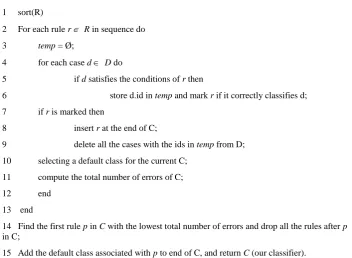
3.3 CBA-CB Basic Steps ... 98
3.4 Summary of the Chapter ... 102
Chapter 4 ... 103
Looking at the Class Associative Classification Algorithm (LC) ... 103
4.1 Introduction ... 103
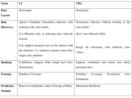
4.2 Main Differences of LC and CBA Algorithms... 104
4.3 The Development of New AC Algorithm ... 105
4.3.1 The Proposed Rule Discovery Algorithm ... 106
4.3.2 Classifier Construction ... 113
4.3.3 Rule Sorting ... 113
4.3.4 Pruning of Rules ... 114
4.3.5 Prediction Method of LC ... 116
4.4 Experimental Environment Setup ... 118
4.4.1 Data Sets Used in Experiments ... 118
4.4.2 Experimental Parameters and Setup ... 119
4.5 Experimental Results and Discussion ... 119
... 129
4.6 Summary of Chapter ... 129
Chapter 5 ... 131
Phishing Data Collection Model and Implementation of LC and other Algorithms ... 131
5.1 Introduction ... 131
5.2 Features Selection for Experiments ... 131
5.2.1 Phishing Data Sources, How and Why Features are Selected ... 132
8
5.3.1 Abnormal Based Features ... 134
5.3.2 Address Bar Based Features ... 135
5.3.3 HTML and JavaScript Based Features ... 136
5.3.4 Domain Based Features ... 137
5.4 Experimental Setup and Data Sets Used ... 138
5.5 Experimental Results and Discussion ... 138
5.6 Summary of the Chapter ... 147
Chapter 6 ... 149
Critical Analysis of the Experimental Results ... 149
6.1 Reduction in the Number of merging of itemsets in LC and its Impact on the Execution time and Memory Usage ... 149
6.2 Total Number of CARs Generated Before and After Pruning ... 150
6.3 Analysis of the Prediction Accuracy Measure ... 152
6.4 Summary of the Chapter ... 154
Chapter 7 ... 155
Conclusions and Future Directions ... 155
7.1 Conclusions ... 155
7.1.1 Issue 1: An Associative Classification Algorithm for Emails and Website Prediction ... 156
7.1.2 Issue 2: Efficiency of Training Phase of AC ... 157
7.1.3 Issue 3 & 4: Prediction Based on Group of Rules and Rule Ranking ... 157
7.1.4 Issue 5: Experimental Study on UCI and Phishing Data Sets ... 158
7.2 Future Directions ... 158
7.2.1 Phishing in Mobile Applications ... 158
9
7.2.3 Noise in Source Databases ... 160
Appendix A ... 162
10
List of Figures
Figure 2.1 Classification as two-step process in data mining ... 28
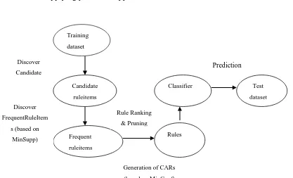
Figure 2.2 Main Steps of an associative classification algorithm ... 51
Figure 2.3 MCAR algorithm ... 60
Figure 2.4 MCAR classifier builder algorithm ... 61
Figure 2.5 Rule discovery algorithm of MCAR ... 61
Figure 3.1 Frequent itemset generation step in CBA algorithm ... 97
Figure 3.2 Building a classifier in CBA algorithm ... 98
Figure 3.3 Rule ranking steps in CBA ... 99
Figure 4.1 Frequent itemset generation step in LC algorithm ... 107
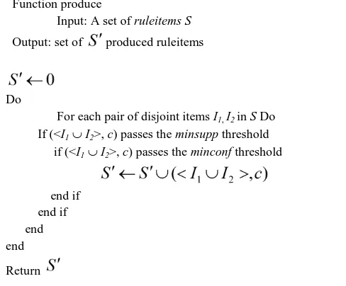
Figure 4.2 Generate candidate ruleitems function and support count calculation in LC algorithm. ... 108
Figure 4.3 Rule ranking in LC algorithm ... 114
Figure 4.4 Classifier building in LC algorithm (database coverage pruning method) ... 115
Figure 4.5 Prediction method in LC ... 117
Figure 5.1 Feature extraction and phishing detection model ... 133
Figure 5.2 No. of merging for all iterations of address bar feature data set of LC and CBA ... 140
Figure 5.3 Total number of itemsets merging of phishing data sets ... 140
Figure 5.4 No. of candidate rules generated for LC and CBA for domain base feature data set 143 Figure 5.5 No. of candidate rules generated for LC and CBA for Abnormal base features ... 143
11
Figure 5.7 Sample for no. of rules generated in C4.5 algorithm for Abnormal base data set ... 145
Figure 5.8 Sample for no. of rules Generated in PART algorithm for HTML and Java Script Base Features data set ... 145
Figure 5.9 Sample for no. of rules Generated in PART for Abnormal Base data set ... 145
Figure 5.10 Sample for no. of rules Generated in C4.5 HTML and Java Script Base Features data set from WEKA ... 145
12
List of Tables
Table 2.1: Lenses data set (UCI machine learning repository) ... 29
Table 2.2 : Test data to advice type of lens ... 30
Table 2.3: Training data ... 54
Table 2.4: Vertical data layout -tid-list ... 55
Table 2.5: Horizontal data layout ... 55
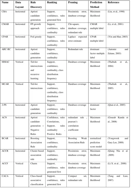
Table 2.6: Summary of AC algorithms ... 95
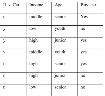
Table 3.1: Training data ... 99
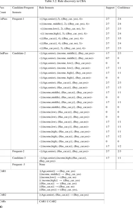
Table 3.2: Rule discovery in CBA ... 100
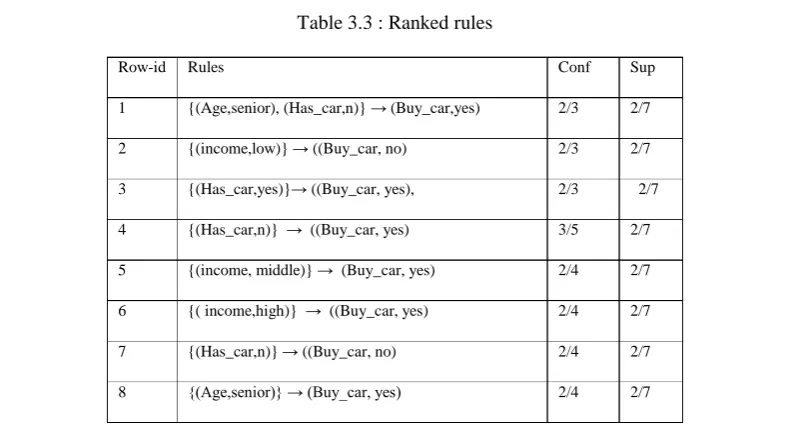
Table 3.3 : Ranked rules ... 101
Table 3.4: Data for testing ... 101
Table 4.1: Main differences between LC and CBA algorithms ... 105
Table 4.2: Training data ... 109
Table 4.3 : LC candidate 1-ruleitems ... 109
Table 4.4: LC candidate 1-ruleitems when minority rule is applied ... 109
Table 4.5: LC frequent 1-ruleitems ... 110
Table 4.6: LC candidate-2 ruleitems ... 110
Table 4.7: Frequent 1-itemsets lkproduced by CBA ... 111
Table 4.8: CBA candidate-2 itemsets ... 111
Table 4.9: Frequent rule itemsets at each iteration with support and confidence counts ... 112
Table 4.10: UCI data sets used in experiments ... 118
Table 4.11: The number of itemsets joining of LC and CBA algorithms ... 121
13
Table 4.13: Physical, paged and virtual memory (bytes) used by CBA and LC algorithms ... 123
Table 4.14: LC and CBA number of CARS and rules generated after pruning, using minSupp=5% and minconf =40% ... 124
Table 4.15: LC and CBA number of rules generated after ... 126
Table 4.16: Comparisons between LC, CBA and C4.5 for prediction accuracy ... 127
Table 4.17: Comparison of single vs group of rule prediction accuracy ... 129
Table 5.1: Comparison of number of merging for the security data sets using minsupp =5% and minconf = 40% ... 139
Table 5.2: Comparisons of number of CARs and candidate rules generated for LC and CBA .. 142
Table 5.3: Number of rules in classifier of AC and classification algorithms ... 144
14
Dedications and Acknowledgements
First of all, I would like to dedicate this research to my ALLAH, whose mercy, blessings and grace has led me to this important moment of my life.
I would like to express my special thanks to my supervisors Dr Fadi Thabtah and Professor Lee McCluskey for their encouragement, patience, support and guidance throughout this research project.
Many many thanks to my father who is always an inspiration for me and mother for her prayers, ongoing support and advice, and my wife, who has been supportive towards me during this period of life.
15
List of abbreviations
AC Associative Classification
AUC Area under the ORC curve
ADT Association based Decision Tree
AREM Associative Classification Regression Model based on EM Algorithm
BART Bayesian Additive Regression Trees
CAEP Classification by Aggregating Emerging Patterns
CART Classification and Regression Trees
CAR Class Association Rule
CBA Classification based on Association Rule
CMAR Classification based on Multiple Class-Association Rules
CPAR Classification based on Predictive Association Rules
DIC Dynamic Itemset Counting
DHP Direct Hashing and Pruning
EP Emerging Patten
ECMC Evolving Clustering method for Classification
FP Frequent Pattern
IREP Incremental Reduced Error Pruning
L3 Live and Let Live
LB Large Bayes
LR Logistic Regression
MCAR Multi-class Classification based on Association Rule
MCMC Markov chain Monte Carlo
MMAC Multi-class, Multi-label Associative Classification
16
PECM Phishing Evolving Clustering Method
PST Prefix Stream Tree
REP Reduced Error Pruning
RF Random Forest
RIPPER Repeated Incremental Pruning to Produce Error Reduction
RMR Ranked Multi-label Rule
17
Chapter 1
Introduction
1.1
Motivation
Storage capabilities have developed tremendously in the past years, hundreds and thousands of files can be saved in a micro memory card. This innovation has tempted and made it feasible for small and large organizations to keep a record of minute details about their customers, like Tesco, ASDA and Morrison’s, etc. in retail market businesses and banks and financial institutions. The transactions of the daily sales in a retail store are often called the market basket data (Agrawal, 1993). The retail stores collect and store the daily purchases and information of all customers. Finding the correlations between the items purchased by the customers and the features of the customers in different geographical areas can be very useful in deciding the marketing strategy and launching targeted promotions.
Assume a planning and marketing department in a retail business organization decided to introduce a store card for their customers. Applications are collected and decisions have to be made for each customer, whether to issue a store card and how much credit limit would be recommended for each customer. The decision from the management of the store needs to take into account the shopping frequency of the customer, geographical area where he lives, and the total amount of purchases in a period of time. These associations can be extracted from the data by the application of data mining approaches.
Another example is a medical organization that keeps the record of all the patients with different diseases and symptoms. The information is very beneficial when the associations are extracted between different symptoms. The extracted information is used to narrow down the possibility of a patient’s disease by entering all the symptoms of a new patient in an automated system. For instance, the data contain a large number of entries with ‘fever’ and ‘shivering’ referring to the possibility of a malarial disease.
18
percentage of transactions containing “smart phone and screen protector” is 3%, and the total transactions of “milk with bread” are 10% in the transactional database. The customers who will buy ‘smart phone’ or ‘milk’ are the antecedent of an association rule and ‘screen protector’ or ‘bread’ is the consequent of the rule. The confidence of a rule represents its strength and in the example above “80% “means that if 100 customers have purchased a smart phone, 80 of them have also bought screen protector. The confidence for the other rule is 60%, whereas “3%” and “10%” represent a significant statistical measure known as support of the rules.
In the real world classification data such as medical diagnoses or market basket analysis, the problem is to discover rules from the data set of historical transactions. The rules generated must have significant support and confidence (frequencies of attribute values above user’s thresholds denoted as minimum support and minimum confidence). A subset of the produced rules is selected to build a model that is able to predict the outcome of the new set of attributes in a database or previously unseen data. The approach that uses association rules to build-up classification systems (classifiers) is known as associative classification (AC) (Li et al., 2001), (Hao et al., 2009), (Sangsuriyu et al., 2010), (Lucas et al., 2012), (Jiang and Karyros, 2012) and (Jabbar et al., 2012).
The AC approaches tend to explore all the linkages or the associations between the values of the attributes (items) and their relative classes in the data set and produce classifiers. The classifiers generated by AC algorithms are usually more accurate with respect to classification accuracy than classic rule based classification approaches like decision trees (Quinlan, 1979) and which tend to generate relatively small size classifiers. The AC approaches have made inroads in extracting such knowledge that is missed by traditional classification methods and have also improved the accuracy rate of different applications.
19
assigning journals to particular category or categories becomes very efficient and convenient when a classifier is set in the automated system.
The process of producing the complete set of rules needs substantial CPU time as it requires many data set scans and itemsets joining during the training phase (Baralis, et al., 2004; Li et al., 2001). Hence it is very important to use a fast and effective method for rule discovery that can improve the training time and memory usage. The classical AC techniques like CBA (Liu et al., 1998) and CBA (2) (Liu et al., 1999) may not be able to deal with the increase in the database size and the dimensions of the datasets, meaning adding more attribute columns in the data base. These techniques produce many rules and the process of rule generation can be complex and exhaustive, because these consider all the attribute values while joining them. Therefore it is essential to derive the rules that will be used in the prediction process in reasonable time and at the same time using less memory resources, to help decision makers to plan without waiting.
Use of AC approaches or techniques are used successfully in real world applications in the recent years like heart disease prediction (Jabbar et al., 2012), based on the data collected from the patients response for treatment of Hepatitis C, (Enas et al., 2012) has implemented a predictive system by using AC approaches and also successful application of AC in artificial immune systems is done by (Samir, 2012).
20
In this thesis, an effective and efficient AC algorithm is proposed for extracting useful knowledge missed by classic rules based classification algorithms for the problem of emails and websites categorization. This is since the proposed algorithm considers efficiently all possible correlations between the websites features and the class in the data set. The proposed algorithm improves upon a known AC algorithm called CBA in three main steps to handle appropriately the problem of websites features prediction:
The training step: Unlike CBA algorithm which employs Apriori (Agrawal, 1993) candidate generation function that works by repeatedly merging disjoint candidate itemsets without considering the class attribute to discover the rules. The proposed algorithm significantly improves the training phase of CBA by reducing the number of itemsets and as a consequence training time as well as memory allocation gets minimized. This has been accomplished by looking at class of candidate disjoint itemsets before merging them and using the minority rule.
Building the classifier phase: The proposed algorithm implements a new ranking method based on the confidence, support, and cardinality, different for the method used by CBA of confidence , support and the order of rule generated. The pruning phase of our algorithm uses the same method of database coverage.
Predicting test data: Unlike the majority of current AC algorithms that use one single rule from the classifier to assign class to test cases. The proposed algorithm makes use of group of rules to make the class assignment of test data. This surely improves upon the classification accuracy of the classifiers produced by the proposed algorithm over other AC algorithms since more rules are cooperating in making the prediction.
1.2
Main Aim of the Thesis
21
Considering all the features in experimental study would be a complex problem, the aim is to select some set of features from the phishing and legitimate websites and extract them by applying some rules. The selected features are then divided into four groups of data sets naming Abnormal Based features, Address Base features, HTML Base features and Domain based features. The classification accuracy of the phishing datasets will be studied and discussed in detail when novel LC algorithm and other AC and classification algorithms are applied.
1.3
Issues Addressed in the Thesis
To achieve the aims of the thesis different issues related to AC mining and the feature selection from the websites are addressed that include the efficiency of the training phase, building the classifier, the prediction phase and the applicability of AC on real world applications such as phishing. These issues will be highlighted here and will be discussed in details in this thesis.
1.3.1 Issue 1: An Associative Classification Algorithm for Emails and Website
Prediction
In this thesis we deal with the problem of automatically categorizing websites and emails to their relevant types based on different features collected and assessed by the proposed AC algorithm. Mainly, the proposed algorithm is developed mainly to successfully allocate the appropriate type of the website based on features related to fake and accurate websites in automated manner. We have developed within the LC algorithm three methods described in the following subsections that have enhanced the primarily the efficiency and the accuracy of the classifiers generated by the LC algorithm when contrasted with known AC and traditional classification algorithms. In other words, we showed the applicability of AC classification as an approach on effectively predict the type of emails and websites in two contexts: classification accuracy and efficiency. Finally, we conducted experiments to extract the useful and important features from the world phishing websites data. Then we compared AC methods as well as traditional classification techniques performance on these data sets to reveal the efficiency and accuracy of LC algorithm.
22
The data used in classification problems is large, and therefore the number of candidate ruleitems
generated also known as potentially frequent ruleitems in each iteration is relatively very large. It is computationally expensive to mine this highly correlated data using AC techniques. To generate the frequent ruleitems it is really essential to have such an algorithm that executes quickly and able to generate rules with minimum use of memory space. Many of the current AC approaches like CBA have adopted the Apriori (Agrawal and Srikant, 1994) candidate discovery step inherited from association rule mining to extract frequent ruleitems. In our thesis “candidate
itemset” and “frequent itemset” terms are used when talking about association rule terms like “candidate ruleitems” and “frequent ruleitems” are used when we mention AC. The discovery of frequent itemsets in Apriori from a transactional data set is achieved in steps, where frequent itemsets discovered in the nth iteration are used to generate potentially frequent itemsets, also known as candidate itemsets at (n+1)th iteration. During the process of each iteration a database scan is necessary to calculate the support and confidence counts of the newly produced candidate itemsets.
Similar to the association rule mining approaches, AC techniques also adopted the concept of Apriori candidate generation function to extract the frequent ruleitems. We enhance the process of finding frequent ruleitems by only considering frequent ruleitems that share common class in the merging process. We also implemented a minority rule method that eliminates all the ruleitems that are associated with the minority classes and keeps the ruleitem
with majority class, if a ruleitem is found linked with more than single class. This substantially minimizes the number of frequent ruleitems produced at the end of rule generation phase, reduces the number of rules in the classifier after pruning phase, and also decreases the training time and reduces memory use.
1.3.3 Issue 3: Enhancing Prediction Procedure of Test Data
23
groups based on their class labels. Then, the average confidences for all rules belonging to the same group are computed and the class that belong to the largest average confidence group gets allocated to the test case. This prediction method ensures that all related rules participate in the class assignment decision.
The classifier by evaluating the candidate rules produced at the training phase against the training data set and only keeping rules that have certain training instances coverage. The process of evaluating each candidate rule on the training data set necessitate that the candidate rule body must exactly match at least one of the training instance. This process of removing rules is carried out in pruning phase thus leading to the improvement in prediction accuracy.
1.3.4 Issue 4: Rule Sorting Criteria
The rules ranking have a significant impact on the prediction step where the top ranked rules are used very frequently to classify test objects. The priority of the rule is usually determined according to several factors such as the support, confidence and the length of a rule (cardinality). In AC, normally a very small support is used and since classification data sets are dense, the expected number of rules with identical support, confidence and cardinality is high.
For example, for “balance-scale” database taken from (Weka, 2000) while keeping
minsupp of 5% and minconf of 40% using the CBA algorithm (Liu, et al., 1998), the classifier have produced 15 rules, having same support values and the top 4 having same confidence value, CBA is not able to discriminate between which rules to select. Furthermore, the 15 rules discovered by CBA also have the same length. So it is harder for CBA to rank them.
24
1.3.5 Experimental Study Comparing Data Mining Approaches on UCI
Many experiments have been conducted while comparing a wide range of classification approaches like decision trees, statistical approaches and AC on different binary and multi-class benchmark problems. We have based our comparisons on accuracy of classification, merging of itemsets during each iteration, execution times and number of rules.
1.4
Outline of Thesis
The thesis comprises of 6 chapters. Chapter 2 describes the data mining with introduction, types of data mining and definitions that will be used in this thesis. Discusses research works performed in association rule and classification techniques in data mining where detailed descriptions of algorithms are given. Chapter 2 also focuses on demonstrating many AC techniques in data mining. It includes the methods used by AC algorithms to produce frequent
ruleitems, discusses the generation of rules, rule sorting and pruning methods and methods for the classifier building and the prediction processes. Chapter 2 also includes the literature review on phishing and use of AC mining in Phishing. Chapter 3 demonstrates the steps and the process of CBA algorithm in detail. The purpose is to explain for the comparison purposes the modifications in CBA algorithm. Chapter 4 introduces the “Looking at the Class (LC) algorithm” for construction of the frequent ruleitems to produce better and efficient classifiers. This chapter presents a fast and effective method to discover frequent ruleitems from databases and demonstrates by experiments its effectiveness and efficiency in terms of number of candidate ruleitems merging and execution time. It and also studies the impact on the performance in terms of accuracy using a number of well-known data sets from UCI. This chapter also proposes new methods for rule ranking and prediction.
25
26
Chapter 2
Literature Review
2.1
Introduction
This chapter is divided mainly into three parts. The first part of the chapter consists of detailed review of two data mining tasks of classification and association rule mining. The differences between these two approaches are highlighted and the benchmark algorithms are discussed in detail for both classification and association rule mining. In the second part of the chapter, third data mining approach which is the combination of both association and classification rule mining, known as associative classification will be presented and lastly in the third part a very important and critical problem of phishing in websites will be discussed in detail. The first part of the chapter demonstrates the classification problem followed by a focus on the classification approaches and will conclude by comparing the research work done in each technique. The benchmark and well known classification approaches such as decision trees (Quinlan, 1986; Quinlan, 1988; Quinlan, 1993; Blackmore and Bossomaier, 2002), Naïve Bayes (Duda and Hart, 1973) and rule induction (Furnkranz, 1999) will be reviewed. The importance of the above techniques discussion is significant as some of them will be used in the comparative analysis of the experimental results in chapter 4 and 5. In the latter half of this part of the chapter the association rule mining technique will be discussed. The association rule mining problem will be presented with the explanation of famous and pioneer rule discovery approaches such as Apriori (Agrawal and Srikant, 1994). This algorithm will be discussed in details because the proposed work has used the basic concept of Apriori rule generation process. The other AR algorithms like FP-growth (Han, et al., 2000), partitioning (Brin, et al., 1997) and others will also be discussed. The main purpose of the discussion is to understand the tasks in classification and rule generation process in Association rule mining before the third type of data mining technique of Associative classification(AC) is discussed.
27
(Jabber et al., 2012), treatment response data in patients of Hepatitis-C (Enas et al., 2012) and artificial immune system (Samir, 2012) will be discussed. Different pruning methods and the current prediction approaches used in AC will be compared and explained in some detail in this part of the chapter.
In the third part of the chapter a very important information security problem called phishing will be introduced. The selection of this important real world problem is due to a fact that the number of web users are increasing in volumes and so as the phishing attacks. An increase of 59% in phishing attack volumes is reported in 2012 than 2011 and globally the losses due to phishing are estimated at $1.5 billion in 2012 an increase of 22% than 2011( RSA’s Report, 2013). The literature is reviewed with emphasis on the use of AC approaches in detecting phishing and different methods been used to extract the features from websites and emails will be discussed in detail.
2.2
Classification Technique in Data Mining
The purpose of classification techniques is to generate rules from a set of training data that contains a set of class labels, and then the model or the set of rules will be used in the prediction of test data while performance metric of accuracy is calculated. Hence the classification is a two stage process as described in Figure 2.1. In the first phase rules are generated by a learning process performed by an algorithm on the training data set. The second phase is the testing of the extracted rules in the first step; these are applied on the test data to predict the outcome of the values in the test data instance.
In classification different approaches for knowledge extraction from a database can be grouped into rule induction separate and conquer (Furnkranz, 1999), divide and conquer (Quinlan, 1987a), statistical approaches (Duda and Hart, 1973; Meretakis and Wüthrich, 1999) and covering (Cendrowska, 1987).
28
[image:30.595.122.483.291.443.2]conquer selects a root node at the top level by using information gain (Quinlan, 1979). The root node contains an attribute from the training data set. The training data set is then split into many subsets depending on the possible values of the attribute selected. The process is iterated until all attributes that are linked in one branch represents the same class or the remaining data entry values are not able to add or split any more. Naïve Bayes is a statistical approach in which all the classes’ probabilities are calculated in the training database. The probabilities are based on the occurrence of associations between the attribute values and used to classify the test data. The rest of the techniques like covering algorithms pick up all the classes present in the data set one by one. In order to extract highly accurate rules, the approaches tries to find a way of covering the maximum number of training instances of that class.
Figure 2.1 Classification as two-step process in data mining
The survey of the classification techniques such as PART (Frank and Witten, 1998), decision trees (Quinlan, 1986; Quinlan, 1993; Quinlan, 1998), Prism (Cendrowska, 1987), RIPPER (Cohen, 1995), and will discuss significance regarding their characteristics and different issues in depth in the next sections.
2.2.1 The Classification Problem
A classification problem is defined as: let ‘D’ denote the data table and ‘C’ as the set of classes present in the table. Each record dD has an outcome in the form of a classcC. The main aim is to find a set of rules known as classifier z:d cthat is able to reduce the chances that z
29
2.2.2 Classification Example
Table 2.1 contains a ‘Lenses’ data set taken from UCI machine learning repository. Depending upon any attribute values of the following attributes: age of patient, spectacle prescription,
astigmatic and tear production rate, the data set ‘Lenses’ is classified into three classes like soft, none and hard. It would be difficult for an optician or eye specialist to advise the type of lens while looking at the data in the above table or a bigger data set. But when the machine learning approaches are applied on the above data, few simple rules are generated that are easy to understand. These rules generated will help any system or the opticians to make their decision such as to advise a new patient about the type of lens. The test data in the Table 2.2 will be classified with the rules generated by classification approaches.
Table 2.1: Lenses data set (UCI machine learning repository)
Age of the Patient Spectacle
Prescription
Astigmatic Tear Production
rate
Class of Lens
young myope no reduced none
young myope no normal soft
young myope yes reduced none
young myope yes normal hard
young hypermetrope no reduced none
young hypermetrope no normal soft
young hypermetrope yes reduced none
young hypermetrope yes normal hard
pre-presbyopic myope no reduced none
pre-presbyopic myope no normal soft
pre-presbyopic myope yes reduced none
pre-presbyopic myope yes normal hard
pre-presbyopic hypermetrope no reduced none pre-presbyopic hypermetrope no normal soft pre-presbyopic hypermetrope yes reduced none pre-presbyopic hypermetrope yes normal none
presbyopic myope no reduced none
presbyopic myope no normal none
presbyopic myope yes reduced none
30
Table 2.2 : Test data to advice type of lens
Age of the Patient Spectacle
Prescription Astigmatic Tear Production rate Class of Lens
young myope yes normal ?
young hypermetrope no normal ?
pre-presbyopic myope yes reduced ?
presbyopic myope yes normal ?
2.3
Common Classification Techniques
2.3.1 Simple One Rule
One rule (OneR) proposed by(Holte, 1993), is a straightforward and cheapest classification approach in which one-level decision tree is constructed and rules are generated from the training records that are linked with frequent classes. The algorithm checks all the existing attributes in the training database and also loops among all different values of each attribute. It then calculates the occurrence of the attribute value in focus with the class value then extracts the frequent class and marks it as a candidate rule. It will count the error rate in classifying the test instances of each rule and stores the rule that have the lesser error rate. The process of finding the association of class with the attribute values continues until no rules left with a desirable error rate.
31
2.3.2 Decision Trees
A very well-known and mostly discussed technique for classification and then used for prediction is decision trees (Quinlan, 1979, 1986, 1998). This approach can be understood by an intellectual’s game of asking some number of questions to guess or identify the place, thing, a personality, or an event from the history or present. Questions are asked in such a fashion that one question is linked and related to the previous question asked. The game starts when one person thinks of any famous thing. A group of intellectual people asks about 15 to 20 questions to reveal the identity of that thing. The series of questions in the above game are represented by decision tree where outcome of one question set up the next question to be asked.
To build a decision tree, from the instance of a data set the attribute is entered in the root node and branches are built for each attribute values that are linked to the root node attribute. This recursive process is continuously applied until all the instances in node have the same class or there is no further room to split the tree (Quinlan, 1979).
When the tree is built, the path from the root node to the end nodes, that is leaf nodes, is termed as a rule. The conditions or antecedent of a rule is the path from the top root node to the leaf node and the consequent of each path is a class attribute value which is assigned by leaf node. The most critical task in this approach is to select a candidate attribute to split or separate the data, because selection affects the class distributions in the branches.
32
2.3.3 ID3 Algorithm
The first decision tree algorithm introduced is ID3 by (Quinlan, 1979). It uses an information gain measure to decide which attribute value should go in the root node. ID3 picks a root node attribute from the available attributes in the training database. As we know that this selection has very crucial impact on the distribution of the classes, so the aim is to select an attribute for the root node with the best information gain value. After the selection is made by the algorithm of the root node, the recursive process of selecting the best attribute in the remaining child nodes continues until the rest of the training data cannot be split further (Utgoff, 1989). A decision tree is constructed after the above process corresponds to an attribute at each node and the arcs contain the attribute’s value. Thus the links in the tree starting from the root node to any leaf node refers to rules.
The information gain information that was used to make a decision regarding placing an attribute in the root node, is also helpful in predicting the class that can or should be assigned to the unclassified test instance.
The attribute which contains the maximum information is selected. The information in an attribute is measured by using Entropy. Give a training data objects D of R rules,
Entropy (D) =
Pjlog2Pj (2.1)wherePj is the probability that D belongs to class j. The information gain of a set of data objects on attribute X is defined as
Information Gain (D, X) = Entropy(D) -
((|Da| / | D|) * Entropy (Da)) (2.2)Where the sum is over each value a of all possible values of attribute X, Da = subset of D for
which attribute X has value a, |Da| = number of data objects in Da, |D| = number of data objects
in D.
A training database D is considered in Table 2.1, which represents ‘Lenses’ information , with three class labels none, soft and hard, D consists of 24 data objects where 15 are associated with class ‘none’, 4 with class ‘hard’ and 5 with class ‘soft’.
33
To calculate the information gain value of attribute Age of the Patient, which contains three attributes values “young” (8/24), “pre-presbyopic” (8/24) and “presbyopic” (8/24).
Gain (T, Age of the patient)=Entropy (T) - (8/24)*Entropy(T(young)+(8/24)*Entropy(T(pre-presbyopic))+ (8/24)*Entropy(T(presbyopic))
The missing attributes should be handled in the ID3 by making some modifications to the algorithm. As the decision tree takes into consideration all the training data attributed values it may produce long paths. Hence pruning is performed to generate a small subset of rules. The extension of the ID3 is done by applying different pruning methods like substituting the sub-tree by the leaf node. The substitution is carried out when the expected error rate in the sub tree is more than the leaf node.
2.3.4 C4.5 Algorithm
C4.5 is a decision tree algorithm that was proposed by Quinlan (Quinlan, 1993), that generates rules from data set. C4.5 is a modification of the ID3 algorithm discussed in the section above 2.3.3. The C4.5 algorithm just like ID3 also uses the information gain measure to determine the root attribute. We will explain in detail in the following section, how C4.5 builds a decision tree. Let the training data set shown in Table 2.1, the algorithm will determine the Entropy for all the four attributes, Age of the Patient, Spectacle Prescription, Astigmatic and Tear Production rate is calculated and one is selected as the root. The process of selection continues in the same fashion for the rest of the attributes. C4.5 also handles the missing values by using the probabilities of the different values representing an attribute. The total numbers of missing values of an attribute are calculated and this value is distributed among the different values of an attribute based on their probabilities, in order to keep the uniformity.
34
new rule can be formed i.e., R by removing some conditions fromR. If the error rate of R is lower than R on the training data set then Ris replaced byR.
2.3.5 Statistical Approach (Naïve Bayes)
Statistical approach uses all the attributes in the training data set to predict the outcome. This approach works unlike the One Rule Algorithm described in section 2.3.1, which finds a best attribute from the training data set which is then used for prediction. The best known statistical algorithm is Naïve Bayes proposed by (Duda and Hart, 1973), it calculates each class probability for an attribute using the combined probabilities of all attribute values of that data object. The algorithm makes an assumption that the conditional probabilities, of the different attributes with the same class, are independent of each other. Thus same weight is given to the training attributes during the calculation of the probabilities with a class. Naïve Bayes algorithm has proven to work well in several experimental studies (Lewis, 1998b; Meretakis and Wüthrich, B, 1999; Friedman, et al., 1997, Dong, at al., 1999).
A training data set is considered in Table 2.1, which describes the patient prescription of a lens. The Naïve Bayes algorithm works by calculating the probabilistic values. The attribute value frequencies in the training data for the age of the patient attribute, we found 8 occurrences of “young” of which 4 instances are associated with class “none”, 2 instances are associated with class “soft” and remaining 2 are with “hard” class from the values in Table 2.1. The probabilistic measure value of each attribute is used to estimate the likelihood.
When a new instance has to be classified of Table 2.2, the probabilistic values of each attribute will be used to predict the likelihood of a class, to be assigned to the test instance. Considering the first test instance from Table 2.2, which contains the values: young, myope, yes and normal, the likelihood of the possible classes is calculated as follow:
Likelihood for class (none) = 4/15 * 7/15 * 8/15 * 3/15 = 0.01327 = 2.42%
Likelihood for class (soft) = 2/5 * 2/5 * 0/5 * 5/5 = 0.16 = 29.18%
Likelihood for class (hard) = 2/4 * 3/4 * 4/4 * 4/4 = 0.375 = 68.40%
From the example above the likelihood for class “hard” is larger than that of class “soft”, and
35
There is one problem in Naïve Bayes algorithm; if an attribute value never occurred for any of the classes in the training data set then the final probability value of an attribute with that class will be zero. A method called Laplace estimator method by (Snedecor and Cochran, 1989) is one solution that adds 1 in the numerator and 3 in the denominator. Another solution is applied by a minute addition to the Naïve Bayes method, a small number say ‘n’ to the numerator and
n/3 to the denominator (Witten and Frank, 2000).
2.3.6 Rule Induction and Covering Approaches
2.3.6.1 Incremental Reduced Error Pruning (IREP)
Incremental Reduced Error Pruning (IREP) technique was proposed by (Furnkranz and Widmer, 1994). It combines the separate and conquer approach with the Reduced Error pruning (REP). REP is an effective method that prunes and generates a set of rules. The errors are estimated at all nodes of the tree by keeping the chunk of training data as a test data that is independent. The process works by estimating the misclassification rate of the test data at each node and is compared with the error if the concerned node is exchanged with the resultant majority class. While replacing the node if the error is reduced, pruning of the sub tree is carried out. This computational and pruning process is performed repeatedly for each node until there is no reduction in error at each node.
IREP works in greedy manner to generate some rules; two sets of data are constructed by random partitioning the training data. One set is growing which contains 66.6% and the rest of training data is considered as pruning set. IREP starts with an empty rule; a rule condition containing the attribute value is added using a Foil-gain metric (Quinlan and Cameron-Jones, 1993). The algorithm appends those conditions to the current rule continuously that increases the Foil-gain value until that rule is not able to cover any data from the growing set. When the rule is constructed, the algorithm then picks one rule from the generated rules and prunes it backwards. From the selected rule IREP deletes one condition and selects that deletion which showed improvement in the function below:
M P
m M p M P m r p r rule v
( , _ , _ , , ) ( )
36
where P,M represents the total number of data instances in the pruning set and r_ p,r_m are the total number of data instances that are predicted by the pruned rule. The pruning process will be continued until a deletion in the rule condition does not improve the value of ‘v’.
The pruned rules are placed in the classifier and the data instances that are linked with it are deleted from both the sets. An empirical study was performed on some benchmark problems which showed that REP is slower than IREP and both are competitive when compared on the basis of error rate (Furnkranz and Widmer, 1994). When compared with C4.5 algorithm, IREP performed well on 16 data sets and showed less error rate, whereas IREP is out performed by C4.5 on 21 data sets.
2.3.6.2 Repeated Incremental Pruning to Produce Error Reduction
RIPPER is a modified version of the IREP algorithm and was proposed by Cohen (Cohen, 1995). RIPPER builds the set of rules called classifier as follows: firstly it divides the training data set like IREP into two parts, a pruning and a growing set. The process starts by an empty rule set and the algorithm appends heuristically one condition at a time till no error is found on the growing set.
The modification in IREP will be explained in this section. One modification is the introduction of revised stopping condition when the rules are generated. In IREP a stopping condition is used that checks the error rate of a learned rule and stops adding rules, when error rate exceeds 50% on the pruned data. This criterion seems to stop too early, if an application domain contains a large number of low coverage rules. RIPPER uses a minimum description length principle (MDL) to stop adding a rule (Rissanen, 1985). When the rule is added the complete description length of the training and the rule data sets is calculated. If the description length is greater than the shortest description length extracted so far, the algorithm will not add any more rules. This technique of MDL considers the best set of rules that reduces the size of the classifier (set of rules) and also minimizes the quantity of information needed to handle the exceptions relating to these set of rules (Witten and Frank, 2000).
37
IREP is again processed through an optimization phase, to further simplify the rule set characteristics.
The RIPPER integrates the IREP and optimization procedures. The working is as follows: A pruned rule pri is selected from the rule set and two alternative rules such as replacement and revision of pri are built. To create the replacement ofpri, an empty rule pri is constructed and pruned to decrease the error rate of the rule set including pri on the pruning data set. And the revision of pri is built in the same fashion but the rule is constructed heuristically and one condition is added at one time to the actual pri instead of the empty rule. The rule with the minimum error rate is selected from these three rules when analysed on the pruning data.
A comparative study is conducted on 36 benchmark data sets (Merz and Murphy, 1996) to estimate prediction accuracy of C4.5, IREP and RIPPER algorithms. The results have revealed that C4.5 has shown less error rates on 15 data sets while RIPPER has demonstrated better values than C4.5 on 20 data sets. On the other hand RIPPER has achieved better results when compared with IREP on 28 data sets.
2.3.7 Prism
Prism is categorized as a covering algorithm to generate classification rules and was proposed by (Cendrowska, 1987). This approach considers one class from the training data and finds a method to cover all the records to that class and the data instances which do not belong to that class are excluded. To achieve the maximum accuracy of the created rules, this approach appends one attribute value to the current rule. At each step, the algorithm selects the condition that increases the probability of the desired classification. The process of rule construction continues until the stopping condition is met. Once a rule is constructed, the algorithm stops building the rules for the current class when all the data associated with the current selected class is covered. After this process another class is selected and so on.
38
has to be added, it requires changing of the complete tree structure (Witten and Frank, 2000). When an instance has to be classified, decision tree uses rules from the tree directly unlike in Prism due to independence of rules, problems may occur when an instance is linked with more than one rule having different classes.
A study was conducted to investigate the e-learning systems while using classification algorithms to produce set of predicting rules for courseware authors in (Romero, et al., 2005). The findings from 50 log files for students have shown that Prism has successfully extracted more accurate rules when compared with ID3.
2.3.8 Hybrid Approach (PART)
PART is a hybrid approach introduced by (Frank and Witten, 1998). Unlike RIPPER and C4.5 approaches that work in two phases, PART produces rules all in one go while avoiding extensive pruning. PART joins both the approaches of divide-and-conquer as in C4.5 and separate-and-conquer as in RIPPER to explore and generate the rules. It constructs a partial decision tree by using divide-and-conquer approach, from the rules generated by separate-and-conquer approach. The PART algorithm avoids building a full decision tree but instead it constructs and prunes a partial decision tree like C4.5. While handling of missing values and pruning approaches remain same as C4.5. PART is different from RIPPER in the pattern of generate rules; each rule in PART refers to the leaf that has the largest coverage in the partial decision tree. On the contrary RIPPER constructs the rule in a greedy fashion, beginning from an empty rule and appends conditions until the rule does not show any error.
The results are gathered from the experimental studied conducted on PART, RIPPER and C4.5 using data sets from (Merz and Murphy, 1996) and have been written in (Frank and Witten, 1998). The results have shown that simplicity of PART has not affected its performance. The set of rules generated are more accurate than RIPPER though they are lengthy, and are also more accurate than C4.5.
39
2.4
Issues in Classification
2.4.1 Over fitting
There are many issues in classification and over fitting is one of them; as the training segment goes on too lengthy with the aim of reducing the error rate to zero, then the general performance of the outcome classifier on test data objects may depreciate. That is called general explanation of the over fitting problem, which can happen due to many reasons like restricted number of training data objects or noise among the training objects (Jensen and Cohen, 2000; Freitas, 2000). In decision tree algorithms for example, it is always possible to create a highly precise decision tree for the training data, but, during the construction of the tree it is generally helpful to stop the building process near the beginning in order to simplify the performance of the result on test data objects. For that reason, pruning approaches like pre-pruning and post-pruning (Breiman, et al., 1984; Quinlan, 1993) have been extensively used during building decision trees to keep away from fitting the training data very well and to give precise performance on test data.
There are many methods exercised to stay away from the problem of overfitting in the classification literature, which includes cross validation (Witten and Frank, 2000) and MDL principle (Rissanen, 1985). Cross validation is a well-recognized evaluation approach in data mining. Cross validation is generally employed when the amount of data for mining is small. In cross validation, the training data set is separated at random into n blocks, every block is held out once, and the classifier is trained on the remaining n-1 blocks; after that its error rate is calculated on the holdout block. Therefore, the learning procedure is executed n times on to some extent different training data sets. When there is enough data, for user then user simply divide the data into two sets, these are training and test. User can discover the classifier from the training set and calculate its quality on the test set.
40
2.4.2 Inductive Bias
Given a training data set, the classification task may be seen as suggest hypotheses (classification rules) from the set of accessible training data objects. Inductive bias can be described as a set of assumptions that lead to the selection of hypothesises (Liu, et al., 2002). With no inductive biases the classification techniques would not be able to help one rule over other ones. In addition, all rules when taken collectively will predict that all data objects are evenly likely, and subsequently cannot supply a basis for prediction.
Classification algorithms are capable to generalise their performance on test data objects by inductive biases because they have contained assumptions of favouring one rule over another. For example, a decision tree algorithms like ID3 (Quinlan, 1979) and C5 (Quinlan 1998) have an obvious bias in their searching for the best attribute decision node, which is, the attribute selection technique based on information gain. Besides, these algorithms help smaller valuable sub-trees over difficult ones by using backward pruning. Probabilistic classification algorithms like Naïve Bayes calculate the probability for every one class in the training data set utilizing joint probabilities of attribute values for a data object. While inductive bias in Naïve Bayes algorithm stands for the assumption that the provisional probability of a data object given a class is independent of the probabilities of other data objects given the same class (Liu, et al., 2002).
At last, because classification algorithms have a bias, the outcomes precision depends a lot on the training data quality. (Freitas, 2000) Just to point out if someone is saying that algorithm X is more accurate than algorithm Y, it is only because of the application domain utilized for the experiment.
2.5
Association Rule Mining
41
the shopping basket items of all the customers. For example, in supermarket transactions, if a customer buys a mobile then what is the probability that he will buy a mobile cover as well? Or if a customer buy a ‘crisps’ what are the chances that he will buy a ‘dip sauce’? And if a customer buys ‘bread’ what is the probability that he will buy a ‘jam’ or ‘butter’? When the business decision makers have the knowledge of association between the frequent sold items, the answer of all the above questions would be much easier. In short the life becomes easy for experts to make strategic decision of buying products, shelving, planning, to launch promotions and advertising. Besides the supermarket example Association rule mining is also helpful in exploring the information in telesales and marketing (Mackinnon and Glick, 1999) , mail ordering (Agrawal and Srikant, 1994) and also in the commerce industry (Pramudiono, et al., 2002).
In association rule mining the task of finding the rules can be described (Agrawal, 1993) in the following points:
Let a data set ‘D’ contain the transactions of sales in a super market, and ITEMS = {item1, item2,
item3, item4, item5………,itemn} is the complete set of items present in the data set ‘D’. Any
transaction ‘T’ in ‘D’ that have any number of non-empty items called an itemset, in such a way
that TITEMS.
An item support is calculated as the total number of occurrence of that item in ‘D’ to the total number of transactions in the data set ‘D.
An itemset containing two or more items, support is calculated as the total number of occurrence of that itemset in ‘D’ to the total number of transactions in the data set ‘D.
An Association rule can be described asitemi itemi1
, where itemi,itemi1 ITEMS and
i1
i item
item
.
The association rule confidence can be defined as or calculated as the proportion of the transactions that contains itemi1 also haveitemi, so to find confidence
) ( support /
)
(itemi itemi1 itemi .
In the association rule approach, inputs of support and confidence values known as minimum support “minsupp” and minimum confidence “minconf” are defined by the users and the problem
42
learning and only itemsets are used to compute the confidence and support values, in contrary to the AC algorithms which considers the class labels with the itemsets to calculate those values in question.
2.5.1 Problem Solving Strategy
The generation of association rules from market basket transactional data set can be divided into two stages as in (Agrawal and Srikant, 1994).
Stage 1: The itemsets that are produced with higher support values than minsupp are known as frequent itemsets and the rest of the itemsets will be termed as not frequent or infrequent.
Stage 2: All the frequent itemsets from above stage 1 will be passed through a check of minconf
value. Those frequent itemsets that have higher value than minconf are kept as rules. rules. The first stage of exploring the frequent itemsets, is comparatively more core and tougher problem than the second stage, and requires exhaustive computation and memory (storage) (Cheung, et al., 1997; Lin and Dunham, 1998; Zaki, et al., 1997; Lim, et al., 2000). We will analyse an example from the same sales records data from a supermarket, suppose that data contains 1050 distinct items; we can image a combination explosion of 21050 possible associations of distinct itemsets, many of them might not be frequent in the next step. We will find only a little subset of frequent itemsets from this huge set of candidate itemsets. This is an extensive research area and many scientists have keenly investigated this problem of exploring frequent itemsets in the past many years. The main aim of the researchers is to improve the efficiency (Bayardo and Agrawal, 1999; Liu, et al., 1999; Li, et al., 1999; Zaki, 2000; Baralis, et al., 2004) in the process of generating frequent itemsets.
In the second stage, the rule generation from the set of explored frequent itemsets is relatively easy process and quiet straight forward, given their support values are already known (Han, et al., 2000).
43
level are carried out with the disjoint frequent 1-items. Apriori works by decreasing the number of candidate items or itemsets at each subsequent level by using a property called as “downward closure”. It is defined as if an itemset has support value greater than the minsupp threshold, then all its subsets have support value greater than minsupp threshold. So it infers that the subset of the frequent itemset will also be frequent and on the contrary the superset of an infrequent itemset is also infrequent. By the introduction of this “downward-closure” property, the numbers of potential itemsets are reduced significantly at each level and thus enhancing the efficiency of the frequent itemset generation process. Many of the algorithms in association rule mining proposed after Apriori uses this “downward-closure” approach.
Approaches that use Apriori have performed efficiently and accurately where the size of the data set is small or the candidate itemsets are less (Liu, et al., 1999; Park et al., 1995). However where the support value is kept low, the number of possible itemsets generated may be huge. Multiple scans over the data set is needed to calculate the itemsets support values at each level of the process, and that leads to a significant computational overhead in respect of execution time and the use of memory. As we all know that the data is being collected on daily basis, all the organizations aim to improve their services to get good profits. As the data is growing, to extract and evaluate this data is also becoming computationally expensive. So the main focal point is to minimize the complexity and our research is aiming for that bit to improve the efficiency in terms of run time without affecting the performance when the data sets are large.
To address the shortcomings in Apriori, different ARM techniques have been introduced like Dynamic Itemset Counting (Brin, et al., 1997), multiple-minimum-support (Liu, et al., 1999), Frequent Pattern Growth (Li, et al., 2000) etc. Some of the approaches will be reviewed and discussed that have achieved some significant improvements in the frequent itemset generation step.