Role of forcing uncertainty and background model error characterization in snow data assimilation

https://doi.org/10.5194/hess-21-2637-2017 © Author(s) 2017. This work is distributed under the Creative Commons Attribution 3.0 License.

Role of forcing uncertainty and background model error

characterization in snow data assimilation

Sujay V. Kumar1, Jiarui Dong2, Christa D. Peters-Lidard3, David Mocko4,1, and Breogán Gómez5

1_{Hydrological Sciences Laboratory, NASA Goddard Space Flight Center, Greenbelt, MD, USA} 2_{I.M. Systems Group Inc., Environmental Modeling Center, NOAA NCEP, College Park, MD, USA} 3_{Hydrosphere, Biosphere and Geophysics, Earth Science Division, NASA Goddard Space Flight Center,}

Greenbelt, MD, USA

4_{Science Applications International Corporation, McLean, VA, USA} 5_{Research to Operations, Met Office, Exeter, UK}

Correspondence to:Sujay V. Kumar (sujay.v.kumar@nasa.gov)

Received: 8 November 2016 – Discussion started: 22 November 2016 Revised: 7 April 2017 – Accepted: 22 April 2017 – Published: 2 June 2017

Abstract. Accurate specification of the model error covari-ances in data assimilation systems is a challenging issue. En-semble land data assimilation methods rely on stochastic per-turbations of input forcing and model prognostic fields for developing representations of input model error covariances. This article examines the limitations of using a single forcing dataset for specifying forcing uncertainty inputs for assimi-lating snow depth retrievals. Using an idealized data assim-ilation experiment, the article demonstrates that the use of hybrid forcing input strategies (either through the use of an ensemble of forcing products or through the added use of the forcing climatology) provide a better characterization of the background model error, which leads to improved data as-similation results, especially during the snow accumulation and melt-time periods. The use of hybrid forcing ensembles is then employed for assimilating snow depth retrievals from the AMSR2 instrument over two domains in the continental USA with different snow evolution characteristics. Over a re-gion near the Great Lakes, where the snow evolution tends to be ephemeral, the use of hybrid forcing ensembles provides significant improvements relative to the use of a single forc-ing dataset. Over the Colorado headwaters characterized by large snow accumulation, the impact of using the forcing en-semble is less prominent and is largely limited to the snow transition time periods. The results of the article demonstrate that improving the background model error through the use of a forcing ensemble enables the assimilation system to bet-ter incorporate the observational information.

1 Introduction

Land data assimilation (DA) methods combine observations of land surface conditions from remote sensing platforms or ground measurements with model forecasts to produce tem-porally and spatially continuous estimates of land surface fields. The merging of the observations and model forecasts is conducted by weighting them appropriately based on their respective sources of errors. As a result, the skill of the DA systems is critically reliant on the accurate specification of errors in observations and model background.

(2008), the specification of input error covariances remains a subjective process in current land data assimilation systems. Ensemble data assimilation techniques such as the ensem-ble Kalman filter (EnKF) are widely used in land data assim-ilation applications (Crow and Wood, 2003; Reichle et al., 2007, 2010; Kumar et al., 2009, 2014; De Lannoy et al., 2012). The EnKF, a Monte Carlo variant of the Kalman filter, uses an ensemble of model trajectories to represent the model error structures. The model error covariance is diagnosed as the sample covariance of the ensemble of model forecasts. The ensemble is typically created by adding stochastic noise to the meteorological forcing, propagated to the model fields through the nonlinear land surface model (LSM). In addi-tion, stochastic perturbations are also commonly applied to the model prognostic fields.

Perturbations are sampled from randomly generated noise and are directly applied to the forcing and model prognos-tic fields. The typical approach is to employ either normally distributed additive perturbations or lognormally distributed multiplicative perturbations, depending on the variable. For example, multiplicative perturbations are normally used for fields such as precipitation, since the use of additive noise could generate unphysical values (less than zero) or consis-tent positive biases during periods where precipitation is ab-sent. In addition, to avoid introducing systematic biases in the perturbed fields, the ensemble mean of the perturbations are normally constrained to zero and one, for additive and multiplicative perturbations, respectively.

In this article, we examine how the reliance on ensem-ble perturbations of forcing fields to develop the background model error impacts the performance of data assimilation. Most land data assimilation systems use a single data source as the forcing input and the input forcing uncertainty is char-acterized by perturbing the meteorological fields from this single data source. The accuracy of the model error covari-ance therefore greatly depends on the accuracy of the forc-ing input (Reichle and Koster, 2003). For example, in a case where precipitation inputs are underestimated, the forcing uncertainty characterized by the resulting ensemble will lead to the underestimation of the model error covariance. In con-trast, alternate strategies, such as the added use of the forc-ing climatology or multiple forcforc-ing data sources, are likely to provide better representations of the forcing uncertainty and a better characterization of the background model error. In this article, we examine the impact of such factors in the context of snow data assimilation case studies.

The article presents two sets of experiments: (1) an ide-alized experiment to demonstrate the impact of model error covariance underestimation and (2) a “real” data assimila-tion scenario, where snow depth retrievals (Oki et al., 2010; Kachi et al., 2013) from the Advanced Microwave Scanning Radiometer 2 (AMSR2) aboard the Global Change Obser-vation Mission – Water (GCOM-W) satellite are used. The assimilation of AMSR2 data is conducted over two differ-ent domains in the contindiffer-ental USA with differdiffer-ent snow

lution characteristics. The different nature of the snow evo-lution in these domains is used to investigate the impact of background model error representations in snow data as-similation. All experiments described in this article are con-ducted using the NASA Land Information System (LIS; Ku-mar et al., 2006), which is an observation-driven land surface modeling and data assimilation system. The data assimilation subsystem in LIS (Kumar et al., 2008) contains algorithms such as the EnKF and supports the assimilation of data from a variety of satellite sensors (Reichle et al., 2010; Liu et al., 2013, 2015; Kumar et al., 2014, 2015, 2016).

2 Ensemble Kalman filter and background error covariance representation

The filtering class of data assimilation algorithms seeks the best estimate of the posterior state conditioned on the past observations, using the statistics of the uncertainties in the model and observations. The Kalman filter (KF) is an opti-mal estimator for linear dynamical systems driven by Gaus-sian noise. The EnKF is a reduced-rank variant of the KF, which assumes normality of model and observation errors and typically requires the use of a small number of ensem-bles to represent these error structures (Reichle, 2008).

EnKF is a sequential data assimilation approach, where the algorithm alternates between a forecast step and an analysis step. In the forecast step, an ensemble of model states is prop-agated forward in time using the LSM. This is followed by an analysis step where the model forecast is updated based on observations. The analysis step is written in the general form as

xa_k=xb_k+Kk[yk−Hkxbk], (1)

wherexb_{is the background model state vector,x}a _{is the}

an-alyzed state vector, y is the observation vector and Hk is

the observation operator that relates the model states to the observations. The subscriptk indicates time and the super-scriptsbandarefer to the state estimates, before and after the update, respectively.Kkis the gain matrix, which represents

the weighting factor that determines the degree to which the model forecast is adjusted towards the observation.Kkis

ex-pressed as

Kk=Pb_kHTk h

HkPb_kHTk +Rk i−1

, (2)

whereRkandPb_kare the observation and forecast model error

covariances, respectively (exponentT refers to the transpose of a matrix). The model error covariance is computed as the sample covariance of the model ensemble.

F1

F1 F1-CLIM

F1 F2

Fn ...

(a) (b) _(c)

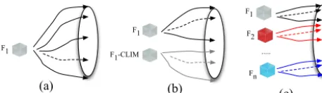
Figure 1.Schematic of the three strategies used to specify forcing uncertainty in the data assimilation integrations:(a)a single forcing dataset,(b)a single forcing dataset and its climatology and(c)an ensemble of forcing products. In all three cases, perturbations are applied to the forcing inputs to generate the ensemble.

the size of the ensemble and the presence of model errors (Li et al., 2009). Prior studies have used techniques such as covariance inflation (Anderson and Anderson, 1999) to deal with the covariance underestimation. These techniques, how-ever, require significant tuning and rely on the assumption that the observation error covariances are known (Miyoshi and Yamane, 2007). In addition, these inflation techniques are ineffective when the model errors are significant and the resulting model error covariances are close to zero. In the ex-amples below, the impact of underestimating the background model error for snow data assimilation is examined.

Figure 1 shows a schematic of three strategies that are used to examine the issue of model covariance underestimation in this article. The first strategy (A), which is the typical prac-tice in land data assimilation systems, is to use a single forc-ing dataset to drive the ensemble. The small perturbations applied to the input forcing variables help in simulating the ensemble spread. In the second strategy (B), the ensemble is forced with both the given forcing and a climatology of that forcing. The added use of the forcing climatology helps in incorporating the representation of average conditions within the ensemble and in reducing the covariance underestimation due to the reliance and limitations of a single dataset. In the third approach (C), the model ensemble is driven using an ensemble of forcing products from different sources, provid-ing a more realistic representation of the input forcprovid-ing uncer-tainty. Note that small perturbations to the forcing variables are also applied to (B) and (C) forcing data to augment the ensemble spread.

3 Assessing the impact of model error covariance underestimation through idealized experiments

In this section, we present an idealized snow depth DA ex-periment to demonstrate the importance of accurately char-acterizing the input model error covariances. We employ snow depth as the measurement variable as most passive microwave retrieval algorithms (Chang et al., 1987; Kelly et al., 2003; Kelly, 2009), compute snow depth first and de-rive the snow water equivalent (SWE) through a climatolog-ical snow density (Brown and Braaten, 1998; Krenke, 1998)

assumption. In addition, most in situ observations of snow are also available as depth measurements, allowing for a more straightforward evaluation of the results from the model and DA integrations. The synthetic experiment is conducted at the Niwot Ridge site in Colorado (40.03◦N, 105.5◦W), which is part of the NRCS Snow Telemetry (SNOTEL) net-work. All model simulations are conducted using the Noah land surface model version 3.3 (Ek et al., 2003). The DA experiment is set up as an identical twin experiment (Ku-mar et al., 2009) with the following structure: first, the Noah LSM is run forced with meteorology from the North Ameri-can Land Data Assimilation System Phase 2 (NLDAS-2; Xia et al. (2012)), and is assumed to represent the “true” state of snow depth evolution at this location. This model integra-tion is termed as the control or “truth” simulaintegra-tion. Next, a set of synthetic snow depth observations is simulated from this control run by introducing realistic retrieval errors. Similar to the strategies used in previous studies (Kumar et al., 2008), to account for the limitations of the passive microwave sensors in retrieving snow depth under dense canopies, the observa-tions are masked out when green vegetation fraction values used in the model are greater than 0.6. In addition, obser-vations are degraded by introducing multiplicative random noise with standard deviation of 0.05 to simulate the errors in the snow depth retrievals. An open loop (OL) integration is conducted using the same LSM, but forced with a different meteorology from the Agricultural Meteorology (AGRMET) model of the US Air Force 557th Weather Wing (formerly the Air Force Weather Agency). A data assimilation integra-tion is then conducted by incorporating the simulated obser-vations into the OL configuration using a one-dimensional EnKF (Reichle et al., 2002). The modeled estimates from the OL and DA integrations are compared against the true fields from the control run to evaluate the impact of assimilation.

An ensemble size of 20 is used in the integrations with per-turbations applied to both meteorological forcing inputs and model prognostic fields to simulate the background model error. Multiplicative perturbations are applied to the precip-itation and downwards shortwave fields with a mean of 1 and standard deviations of 0.3 and 0.5, respectively. Additive perturbations with a standard deviation of 50 W m−2are ap-plied to the long-wave radiation fields. The Noah LSM model fields of SWE and snow depth are perturbed with multiplica-tive noise of 0.01 and 0.02, respecmultiplica-tively. Time series correla-tions are imposed via a first-order regressive model (AR(1)) with a timescale of 24 h for forcing variables and 12 h for the model fields. The perturbations to the forcing fields are applied hourly, whereas the model prognostic fields are per-turbed at 3 h intervals, similar to the configurations used in Kumar et al. (2015, 2014).

0 100 200 300 400 500 600

2012/09 2012/10 2012/11 2012/12 2013/01 2013/02 2013/03 2013/04 2013/05 2013/06

Snow depth (mm)

Control OL_FSNGL DA_FSNGL OBS

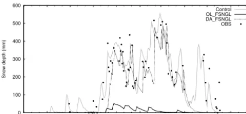
Figure 2. Snow depth time series for the water year of 2012–

2013 from the open loop (OL_FSNGL) and data assimilation (DA_FSNGL) integrations using a single forcing dataset, for the synthetic snow data assimilation experiment. The control simula-tion and the simulated observasimula-tions are also shown.

similates observations into the OL_FSNGL configuration (DA_FSNGL). Note that the OL_FSNGL configuration in-cludes the ensemble perturbations to the forcing and model state fields, to exclude any changes in model skill intro-duced by the perturbations in the evaluation of the DA re-sults. The control and OL_FSNGL runs are significantly dif-ferent in their simulation of snow depth for this winter sea-son. The OL_FSNGL-based snow depth estimates vastly un-derestimate the snow evolution, likely due to the underesti-mation of precipitation in the AGRMET data at this loca-tion. The assimilation of the observations helps in signifi-cantly improving the OL_FSNGL representation, especially during the peak winter months of January through March. The simulation of snow depth during the snow accumula-tion time periods and the snowmelt time periods, however, shows significant differences relative to the control simula-tion, though synthetic observations of snow depth exist dur-ing these time periods. As shown in Fig. 2, the snow accumu-lation in the OL_FSNGL simuaccumu-lation is significantly delayed relative to the control. The input model error covariances (Pbk_{), therefore, remain close to zero until mid-December}

2012, when non-zero snow depth estimates are observed in the OL_FSNGL configuration. These model errors result in the gain matrix (Kk) being zero when the background model

error variances are zero. As a result, no non-zero analysis in-crements are generated from the DA analysis and no changes in the snow depth fields from DA are observed until mid-December, 2012. In contrast, during the peak winter months, the snow depth estimates from DA_FSNGL are closer to the control simulation, as the availability of a non-zero model error covariance allows DA to compute positive analysis in-crements. Further, the DA_FSNGL integration also fails to capture the late season snow events (late April and early May 2013), as the deficiencies in the background model error re-sult in the inability of the analysis step to produce meaningful analysis increments.

In the above example, the main source of the model defi-ciencies is the errors in the forcing inputs, as the same model

is used in the control and open loop integrations. Two vari-ants of this experiment are conducted by (1) using the forcing climatology in combination with the input forcing to spec-ify the ensemble (EXP-FCLIM) and (2) using an ensemble of forcing datasets to drive the ensemble (EXP-FENS). A climatological forcing dataset is developed by averaging the forcing inputs (used in OL_FSNGL) at each forcing time step across 4 years (2012 to 2015). In EXP-FCLIM, the forcing climatology is used to drive 10 of the 20 ensemble mem-bers with the remaining 10 driven by the OL_FSNGL forcing data. In EXP-FENS, four different forcing datasets (different from the data used in the control) are used to drive the model ensemble. The forcing products used in EXP-FENS include the Global Data Assimilation System (GDAS; Derber et al., 1991) operational outputs from NOAA/NCEP, the Modern Era Retrospective analysis for Research and Applications, version 2 (MERRA-2; Bosilovich et al., 2017) data, the Eu-ropean Center for Medium Weather Forecasting (ECMWF; Molteni et al., 1996) and AGRMET datasets. Each forcing data are used to drive five ensemble members within the 20 member ensemble. As before, perturbations are applied to both forcing and model states. These strategies assume that a better representation of the forcing uncertainty and model er-ror covariance can be developed by augmenting the ensemble through the use of multiple data sources.

Panel (a) in Fig. 3 shows the time series of snow depth from open loop and DA integrations from the EXP-FCLIM and EXP-FENS experiments, panel (b) shows comparisons of the snow depth ensemble spread from DA integrations and panel (c) shows comparisons of the analysis increments in snow depth from DA. In the EXP-FCLIM experiment, it can be noted that the added use of forcing climatology with the OL_FSNGL forcing is helpful in increasing the en-semble spread in the DA integrations without a significant change to the mean snow-depth estimates. Subsequently, the improved background model error representation leads to improved DA performance, as the DA_FCLIM-based esti-mates are improved relative to the DA_FSNGL estiesti-mates. The improvements are more apparent during the snow ac-cumulation (December–January) and melt (April–May) time periods, though they are significantly underestimated rela-tive to the control. Quantitarela-tively, the root mean square er-ror (RMSE) in the OL_FSNGL and OL_FCLIM integrations for the Oct 2012 to Jun 2013 time period is 85 mm. The DA_FSNGL integration with a single forcing dataset has a RMSE of 55 mm and the added use of the forcing ensemble helps in further reducing the overall RMSE to 48 mm in the DA_FCLIM integration.

simulations (DA_FENS), as it shows a closer match with the control relative to all other DA integrations. In partic-ular, DA_FENS shows improvements in the accumulation (November–December) and snowmelt (March–April) peri-ods, and provides a low RMSE of 29 mm, for the time period of Oct 2012 to June 2013.

Comparisons of the analysis increments from DA inte-grations shown in panel (c) indicate the time periods where the impact of the background model error is more signifi-cant. Generally, the analysis increments from DA_FSNGL and DA_FCLIM are similar, except during the snow accu-mulation and melt-time periods. Comparatively, larger dif-ferences in the analysis increments between the DA_FSNGL and DA_FENS integrations are observed, with more promi-nent differences seen during the accumulation and melt pe-riods. During these times, larger analysis increments are ob-served in the DA_FCLIM and DA_FENS integrations, re-flective of the ability of these configurations to respond to observations due to the improved background model error. It can also be noted that the analysis increments during the peak snow season are generally smaller in DA_FENS and DA_FCLIM integrations compared to that of DA_FSNGL, indicating the contribution of the hybrid forcing inputs for reducing the significant biases in the assimilation system.

4 Impact of forcing ensemble in the assimilation of AMSR2 snow depth retrievals

The idealized experiments presented in the previous sec-tion demonstrate that the use of hybrid forcing ensemble strategies is helpful in providing a better characterization of the forcing uncertainty and the background model error. We extend this approach to a “real” data assimilation scenario where passive microwave snow depth observations from the AMSR2 instrument are employed. These retrievals, avail-able from 2012 July onwards, are obtained from the Japan Aerospace Exploration Agency (JAXA; http://suzaku.eorc. jaxa.jp/GCOM_W/data/data_w_index.html). In all the inte-grations assimilating AMSR2 retrievals, the standard devia-tion of the observadevia-tion error is assumed to be 50 mm. Note that we use a higher value of observation error standard de-viation than that reported by Kachi et al. (2013), based on the previous snow DA studies (Liu et al., 2013, 2015; Kumar et al., 2014, 2015) that generally assume low skill for passive microwave snow depth retrievals.

Land surface model simulations using the Noah LSM (ver-sion 3.3) are conducted over two regional model domains in the continental USA (Fig. 4) at 25 km spatial resolution: (1) a region centered around the Great Lakes (GL) and (2) a do-main centered around the Colorado headwaters (CH). The snow evolution in the GL region tends to be ephemeral, wet and shallow, whereas the CH region is a high-terrain domain with complex topography and large seasonal snowpacks. The impact of different background model error representations

-300 -200 -100 0 100 200 300 400

2012/09 2012/10 2012/11 2012/12 2013/01 2013/02 2013/03 2013/04 2013/05 2013/06

o

w depth analysis increment

s DA_FSNGL DA_FENS -300 -200 -100 0 100 200 300 400

2012/09 2012/10 2012/11 2012/12 2013/01 2013/02 2013/03 2013/04 2013/05 2013/06

o

w depth analysis increment

s DA_FSNGL DA_FCLIM 0 20 40 60 80 100 o

w depth ensemble spread(

m DA_FSNGL DA_FENS 0 20 40 60 80 100 o

w depth ensemble spread(

m DA_FSNGL DA_FCLIM 0 100 200 300 400 500 600

Snow depth (mm)

Control OL_FSNGL DA_FSNGL OL_FCLIM DA_FCLIM OBS 0 100 200 300 400 500 600

Snow depth (mm)

Control OL_FSNGL DA_FSNGL OL_FENS DA_FENS OBS S now de pt h (m m ) S now de pt h (m m ) EXP-FCLIM (b) EXP-FENS (b) EXP-FCLIM (a) EXP-FENS (a) S now de pt h ana lys is inc re m ent s (m m ) S now de pt h ens em bl e spre ad (m m ) EXP-FCLIM (c) EXP-FCLIM (c) S now de pt h ana lys is inc re m ent s (m m ) S now de pt h ens em bl e spre ad (m m )

Figure 3.Similar to Fig. 2, with the time series of model simula-tions from EXP-FCLIM and EXP-FENS included(a). The FCLIM experiments employ the use of a single forcing dataset and its cli-matology to force the ensemble and the FENS experiments employ the use of an ensemble of forcing datasets. The time series in(b)of the top and bottom figures compares the ensemble spread from the DA_FCLIM and DA_FENS integrations to the ensemble spread of DA_FSNGL integration, respectively. Panel(c)shows comparison of the analysis increments from DA integrations.

on the assimilation of AMSR2 data is examined over these two domains with contrasting snow development and melt characteristics.

MERRA-Figure 4.Two study domains with the 1 km terrain elevation (m) as the background:(a)GL domain and(b)CH domain. The yellow circles indicate the locations of the grid cells used for time series comparisons.

2 datasets. The LSM simulations are conducted during a time period of October 2012 to December 2015 with a time step of 30 min.

We focus first on the GL region by comparing the snow evolution from various model and data assimilation inte-grations. Figure 5 presents a “RMSE improvement” map (RMSE of DA with the single forcing (DA_FSNGL) mi-nus the RMSE of DA with the hybrid forcing ensemble (DA_FCLIM or DA_FENS)) by comparing to the in situ snow depth measurements at the Global Historical Climate Network (GHCN; Menne et al., 2012) sites. The available station observations are aggregated up to the model reso-lution through simple averaging in these comparisons. The warm colors indicate locations where the DA_FCLIM or DA_FENS has a reduced RMSE compared to DA_FSNGL and the cool colors indicate locations where DA_FSNGL has an increased skill relative to DA_FCLIM or DA_FENS. As the figure indicates, the DA integrations employing hybrid

forcing inputs are systematically better than the DA_FSNGL simulation in most parts of the domain. Comparatively, the RMSE improvements are larger in the DA_FENS integra-tion than the DA_FCLIM simulaintegra-tion. Note that the improved skill of DA_FENS in particular, is benefited by both the im-proved model background and the skill of the precipitation data sources that constitute the forcing ensemble, though it is hard to separate their contributions. This is demonstrated by comparing the time series of model and DA simulations at two locations: point A, at 45.875◦N, 89.375◦W and point B, at 48.875◦N, 97.625◦W.

underesti-RMSE (DA_FSNGL) - underesti-RMSE (DA_FCLIM)

RMSE (DA_FSNGL) - RMSE (DA_FENS) °

°

° °

° °

° °

° °

° °

Figure 5.RMSE (mm) differences of snow depth fields from DA

integrations using hybrid ensemble forcing strategies (DA_FCLIM and DA_FENS) relative to the DA integration using a single forcing (DA_FSNGL) over the Great Lakes domain, using GHCN data as the reference, for the time period of 2012 to 2015. Warm colors in-dicate locations where DA_FCLIM or DA_FENS provides a lower RMSE than DA_FSNGL and cool colors indicate locations where DA_FSNGL has a lower RMSE than DA_FCLIM or DA_FENS.

mation (especially during the early snow season), but fails to capture the late season snow events. The AMSR2 retrievals at this location are primarily available in the late snow sea-son and help in improving the snow depth simulation through DA. Overall, the limitations of the OL_FSNGL prevents DA from making a significant impact in the DA_FSNGL simulation. The availability of the improved background in DA_FCLIM and DA_FENS enables them to provide a bet-ter match to the relatively large snow events in March and April, compared to other simulations. Table 1 shows a sum-mary of the cumulative RMSE from various simulations at these locations. The cumulative RMSE from the OL_FSNGL is 381 mm, which reduces to 275 and 169 mm with the OL_FCLIM and OL_FENS, respectively. The cumulative RMSE in the DA integrations is 266 mm for DA_FSNGL, 262 mm in DA_FCLIM and 244 mm in DA_FENS. Note that the cumulative RMSE does not reflect the obvious improve-ment during the late season snow periods in DA_FENS (over OL_FENS), as the early season underestimation dominates these statistics.

Figure 6b shows a similar time series comparison at point B with larger snow evolution. Similar to point A, OL_FSNGL underestimates the snow evolution throughout the season (RMSE of 252 mm) and is improved by the use of the hybrid forcing ensembles. During the snow accumulation time periods (up to early February 2013), the OL_FCLIM (RMSE of 201 mm) and OL_FENS (RMSE of 167 mm) es-timates show better agreement with the GHCN measure-ments. The AMSR2 retrievals show significant underestima-tion relative to GHCN during the peak snow season, though they are helpful in improving the snow depth simulations in

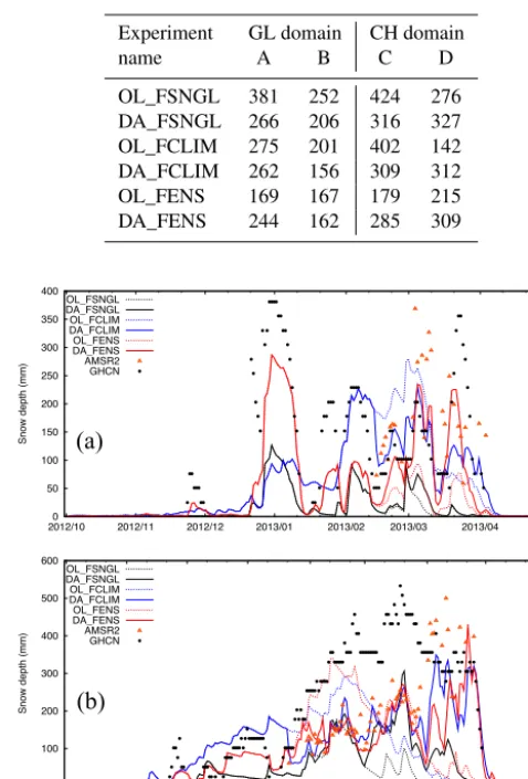
Table 1.Cumulative RMSE (mm) from various model and DA

in-tegrations at the four locations in the Great Lakes and Colorado headwaters domains used in the Figs. 6 and 8.

Experiment GL domain CH domain

name A B C D

OL_FSNGL 381 252 424 276

DA_FSNGL 266 206 316 327

OL_FCLIM 275 201 402 142

DA_FCLIM 262 156 309 312

OL_FENS 169 167 179 215

DA_FENS 244 162 285 309

(a)

(

b

)

2012/10 2012/11 2012/12 2013/01 2013/02 2013/03 2013/04 2013/05

Snow depth (mm)

OL_FSNGL DA_FSNGL OL_FCLIM DA_FCLIM OL_FENS DA_FENS AMSR2 GHCN

0 100 200 300 400 500 600

2012/10 2012/11 2012/12 2013/01 2013/02 2013/03 2013/04 2013/05

Snow depth (mm)

OL_FSNGL DA_FSNGL OL_FCLIM DA_FCLIM OL_FENS DA_FENS AMSR2 GHCN

Figure 6. Time series of snow depth fields at location A (a)

and B (b) from model open loop (OL_FSNGL, OL_FCLIM and OL_FENS), data assimilation (DA_FSNGL, DA_FCLIM and DA_FENS), AMSR2 and in situ (GHCN).

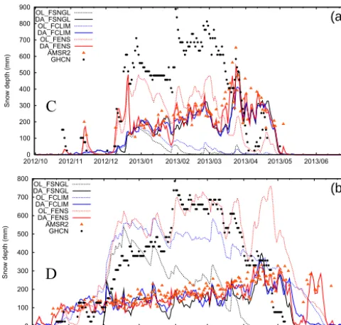
in the CH domain. In addition, larger improvements and degradations are observed in the DA_FCLIM and DA_FENS integrations relative to DA_FSNGL. To examine these pat-terns, the time series of snow evolution from various in-tegrations is compared at two locations in the CH domain (point C at 40.375, 106.875 and point D at 45.125, 109.875) and are shown in Figure 8. OL_FSNGL underestimates the snow evolution in both locations (RMSE of 424 and 276 mm at C and D, respectively, as shown in Table 1). The added use of the climatology (OL_FCLIM) marginally improves the snow simulation at location C (RMSE of 402 mm) and pro-vides more significant improvements at location D (RMSE of 142 mm). The use of the forcing ensemble (OL_FENS) provides a better match to the observations at location C (RMSE of 179 mm), but overestimates the snow accumula-tion at locaaccumula-tion D (RMSE of 215 mm). At locaaccumula-tion C, the as-similation of AMSR2 improves the snow depth estimates in DA_FSNGL (RMSE of 316 mm) and DA_FCLIM (RMSE of 309 mm) integrations relative to their respective OL, whereas DA leads to degradations in the forcing ensemble configu-ration (RMSE of 285 mm), compared to OL_FENS. At lo-cation D, the assimilation of AMSR2 retrievals leads to in-creased RMSE in the DA integrations (RMSE of 327, 312 and 309 mm for DA_FSNGL, DA_FCLIM and DA_FENS, respectively). These trends are reflective of the fact that the AMSR2 observations underestimate the snow evolution in the peak winter months (January–March) and overestimates snow estimates in the spring melt-time periods (April–May), at location C. At location, D, however, the AMSR2 snow observations are generally underestimated. The underesti-mation of snow at both these locations is likely due to the fact that passive microwave-based retrievals saturate for thick snowpacks (Dong et al., 2005).

In general, the DA integrations (DA_FSNGL, DA_FCLIM and DA_FENS) have comparable performance at both these locations and they mostly follow the snow evolution patterns in the AMSR2 data. Note that though AMSR2 observations capture the seasonality of snow observations, they show sig-nificant underestimation compared to in situ observations of snow depth. The influence of undersampling the background model error can be observed in the early part of the snow season at location C and during late season at location D, where the DA_FSNGL integrations fail to match the snow events captured by AMSR2. During the peak snow time peri-ods, however, the undersampling of background model error in OL_FSNGL is less of a problem over this domain, as the non-zero model snow states provide an adequate background for subsequent data assimilation updates. Thus, the evalua-tion of the snow DA integraevalua-tions at these two regions provide valuable insights on the importance of accurately character-izing the background model error. The use of the hybrid forc-ing ensemble and improved model background is more help-ful over the GL domain, where snow evolution is ephemeral. Over regions with large snowpacks such as the CH region, the representation of the model background is more

impor-RMSE (DA_FSNGL) - impor-RMSE (DA_FENS) RMSE (DA_FSNGL) - RMSE (DA_FCLIM)

°

°

°

° ° ° °

° °

° °

° ° °

Figure 7.Same as Fig. 5, but for the Colorado headwaters domain.

tant during the early accumulation and spring melt-time pe-riods.

5 Summary

Accurate specification of input model and observations er-ror covariances in data assimilation systems is challenging though these error specifications are critical in the develop-ment of a skillful data assimilation system. In offline ensem-ble land data assimilation systems, the model ensemensem-ble and background model error representation are typically gener-ated by applying small perturbations to the model prognostic states and input meteorological forcing fields. Most Land DA studies are reliant on the use of a single forcing dataset to de-rive their driving meteorology.

C

D

0 100 200 300 400 500 600 700 800

2012/10 2012/11 2012/12 2013/01 2013/02 2013/03 2013/04 2013/05 2013/06

Snow depth (mm)

OL_FSNGL DA_FSNGL OL_FCLIM DA_FCLIM OL_FENS DA_FENS AMSR2 GHCN 0 100 200 300 400 500 600 700 800 900

2012/10 2012/11 2012/12 2013/01 2013/02 2013/03 2013/04 2013/05 2013/06

Snow depth (mm)

OL_FSNGL DA_FSNGL OL_FCLIM DA_FCLIM OL_FENS DA_FENS AMSR2 GHCN

(a)

(b)

Figure 8. Time series of snow depth fields at location C (a)

and D (b) from model open loop (OL_FSNGL, OL_FCLIM and OL_FENS), data assimilation (DA_FSNGL, DA_FCLIM and DA_FENS), AMSR2 and in situ (GHCN).

is examined in the context of snow data assimilation. When significant errors are present in the forcing fields (e.g., pre-cipitation), the resulting model and ensemble estimates will have significant errors. In such instances, the use of an en-semble of forcing datasets, either based on climatology or a suite of independent datasets, is likely to provide a better representation of the forcing uncertainty and the background model error. This article demonstrates these issues through both idealized and real data assimilation experiments.

The idealized experiment presents a case where the snow depth estimates are significantly underestimated due to the presence of precipitation biases. The application of stochas-tic perturbations using this biased precipitation input is inad-equate in providing a realistic background model error in the assimilation system. As a result, the snow depth fields in the DA system remain biased, especially during the snow evolu-tion and spring melt periods. In contrast, when an ensemble of forcing datasets is used to drive the model, the represen-tation of the background model error is more realistic. As a result, the assimilation system performs better in incorporat-ing the impact of observations durincorporat-ing the snow evolution and ablation periods.

The impact of using a forcing ensemble for developing the background model error is examined for the assimilation of snow depth retrievals from the AMSR2 instrument, over two domains in the Continental USA with different snow evolu-tion characteristics. Over the region near the Great Lakes, the snow evolution tends to be shallow, with transitions between snow and no-snow conditions during each snow season. In

this region, the added use of the forcing climatology to drive the ensemble leads to improved DA performance, when com-pared to the in situ ground observations of snow depth. The DA performance is further enhanced with the use of an en-semble of forcing inputs, partly aided by the enhanced skill of the precipitation inputs. Over the Colorado headwaters, an area with large seasonal snowpacks, the impact of precipita-tion biases on the simulaprecipita-tion of snow states is largely lim-ited to the snow evolution and ablation time periods. As the occurrences of transitions between snow and no-snow states are less common during the peak winter months in this re-gion, the underestimation of the background model error is less problematic in the DA integrations during these time pe-riods. As a result, the positive impact of the use of forcing ensemble is mostly prominent during the accumulation and ablation time periods.

As noted above, the evaluation of snow depth estimates over CH region shows mixed results, with several locations indicating a worse performance with the use of the forcing ensemble compared to the use of a single forcing dataset. In regions with large snow accumulation (such as the CH region), passive microwave retrievals such as those from AMSR2 are known to have low skill due to issues such as saturation in deep snowpacks, signal loss in wet snow and overestimation in the presence of large snow grains (Dong et al., 2005; Foster et al., 2005; Durand et al., 2011). Such limitations contribute to the mixed results seen in these re-sults, especially in the CH domain. In such instances, the poorer performance from the use of the forcing ensemble is a result of the poor skill of the retrievals. To improve the skill of the retrievals themselves, prior studies (Kumar et al., 2014; Liu et al., 2015) have successfully employed objective analysis techniques such as optimal interpolation to blend in situ measurements with satellite retrievals prior to assimila-tion. These prior studies and the results of this article suggest that a strategy that combines the use of hybrid forcing inputs (to improve background model error) and in situ data-based correction of observations to be assimilated (to enhance the satellite retrievals) is likely to provide a robust configuration for optimal DA performance.

may be practical in operational assimilation environments for centers with ensemble prediction systems. Where not avail-able, the combined use of the forcing climatology along with the single, operational forcing input may be an appropriate strategy to improve the skill of the data assimilation system, as validated by the results in this paper.

Data availability. The citations to the datasets are included in the manuscript, which also provide information about their access and distribution. The NLDAS-2 forcing data used in this effort were ac-quired as part of the activities of NASA’s Science Mission Direc-torate, and are archived and distributed by the Goddard Earth Sci-ences (GES) Data and Information Services Center (DISC).

Competing interests. The authors declare that they have no conflict of interest.

Acknowledgements. Funding for this work was provided by the NOAA’s Climate Program Office (MAPP program). Computing was supported by the resources at the NASA Center for Climate Simulation. We are grateful to Andrew Newman and an anonymous reviewer for their valuable edits and suggestions to the manuscript.

Edited by: M. Bernhardt

Reviewed by: A. Newman and one anonymous referee

References

Anderson, J. and Anderson, S.: A Monte Carlo implementation of the nonliner filtering problem to produce ensemble assimilations and forecasts, Mon. Weather Rev., 127, 2741–2758, 1999. Bosilovich, M. G., Robertson, F. R., Takacs, L., Molod, A.,

and Mocko, D.: Atmospheric Water Balance and Variabil-ity in the MERRA-2 Reanalysis, J. Climate, 30, 1177–1196, https://doi.org/10.1175/JCLI-D-16-0338.1, 2017.

Brown, R. and Braaten, R.: Spatial and temporal variability of Canadian monthly snow depths, Atmos. Ocean, 36, 37–54, https://doi.org/10.1080/07055900.1998.9649605, 1998. Chang, A., Foster, J., and Hall, D.: Nimbus-07 SMMR derived

global snow cover parameters, Ann. Glaciol., 9, 39–44, 1987. Crow, W. and Wood, E.: The assimilation of remotely sensed soil

brightness temperature imagery into a land surface model us-ing ensemble Kalman filterus-ing: A case study based on ESTAR measurements during SGP97, Adv. Water Resour., 26, 137–149, 2003.

De Lannoy, G., Reichle, R., Arsenault, K., Houser, P., Kumar, S., Verhoest, N., and Pauwels, V.: Multi-scale assimilation of AMSR-E snow water equivalent and MODIS snow cover frac-tion observafrac-tions in Northern Colorado, Water Resour. Res., 48, W01522, https://doi.org/10.1029/2011WR010588, 2012. Dee, D.: On-line estimation of error covariance parameters for

at-mospheric data assimilation, Mon. Weather Rev., 123, 1128– 1145, 1995.

Derber, J. and Bouttier, F.: A reformulation of the background er-ror covariance in the ECMWF global data assimilation system, Tellus, 51, 195–221, 1999.

Derber, J. C., Parrish, D., and Lord, S.: The new global operational analysis system at the National Meteorological Center, Weather Forecast., 6, 538–547, 1991.

Dong, J., Walker, J., and Houser, P.: Factors affecting remotely sensed snow water equivalent uncertainty, Remote Sens. Envi-ron., 97, 68–82, 2005.

Durand, M., Kim, E., Margulis, S., and Molotch, N.: A first order characterization of errors from neglecting stratig-raphy in forward and inverse passive microwave mod-eling of snow, IEEE Geosci. Remote S., 8, 730–734, https://doi.org/10.1109/LGRS.2011.2105243, 2011.

Ek, M., Mitchell, K., Yin, L., Rogers, P., Grunmann, P., Koren, V., Gayno, G., and Tarpley, J.: Implementation of Noah land-surface model advances in the NCEP opera-tional mesoscale Eta model, J. Geophys. Res., 108, 8851, https://doi.org/10.1029/2002JD003296,296, 2003.

Foster, J., Sun, C., Walker, J., Kelly, R., Chang, A., Dong, J., and Powell, H.: Quantifying the uncertainty in passive microwave snow water equivalent observations, Remote Sens. Environ., 94, 187–203, 2005.

Huang, C., Newman, A. J., Clark, M. P., Wood, A. W., and Zheng, X.: Evaluation of snow data assimilation using the en-semble Kalman filter for seasonal streamflow prediction in the western United States, Hydrol. Earth Syst. Sci., 21, 635–650, https://doi.org/10.5194/hess-21-635-2017, 2017.

Kachi, M., Naoki, K., Hori, M., and Imaoka, K.: AMSR2 valida-tion results, in: 2013 IEEE Internavalida-tional Geoscience and Remote Sensing Symposium-IGARSS, 831–834, 2013.

Kelly, R.: The AMSR-E snow depth algorithm: Description and ini-tial results, Journal of the Remote Sensing Society of Japan, 29, 307–317, 2009.

Kelly, R. E., Chang, A. T., Tsang, L., and Foster, J. L.:

A prototype AMSR-E global snow area and snow

depth algorithm, IEEE T. Geosci. Remote, 41, 230–242, https://doi.org/10.1109/TGRS.2003.809118, 2003.

Krenke, A.: Former Soviet Union hydrological snow surveys, 1966-1996. Edited by NSIDC, Digital media, National Snow and Ice Data Center/World data center for glaciology, updated 2004, 1998.

Kumar, S., Peters-Lidard, C., Tian, T., Houser, P., Geiger, J., Olden, S., Lighty, L., Eastman, J., Doty, B., Dirmeyer, P., Adams, J., Mitchell, K., Wood, E., and Sheffield, J.: Land information sys-tem: An interoperable framework for high resolution land surface modeling, Environ. Modell. Softw., 21, 1402–1415, 2006. Kumar, S., Reichle, R., Peters-Lidard, C., Koster, R., Zhan, X.,

Crow, W., Eylander, J., and Houser, P.: A land surface data as-similation framework using the Land Information System: De-scription and Applications, Adv. Water Resour., 31, 1419–1432, https://doi.org/10.1016/j.advwatres.2008.01.013, 2008. Kumar, S., Reichle, R., Koster, R., Crow, W., and Peters-Lidard,

C.: Role of subsurface physics in the assimilation of surface soil moisture observations, J. Hydrometeorol., 10, 1534–1547, https://doi.org/10.1175/2010JHM1262.1, 2009.

mois-ture data assimilation, Water Resour. Res., 48, W03515, https://doi.org/10.1029/2010WR010261, 2012.

Kumar, S., Peters-Lidard, C., Mocko, D., Reichle, R., Liu, Y., Arse-nault, K., Xia, Y., Ek, M., Riggs, G., Livneh, B., and Cosh, M.: Assimilation of remotely sensed soil moisture and snow depth retrievals for drought estimation, J. Hydrometeorol., 15, 2446– 2469, https://doi.org/10.1175/JHM-D-13-0132.1, 2014. Kumar, S., Peters-Lidard, C., Arsenault, K., Getirana, A.,

Mocko, D., and Liu, Y.: Quantifying the added value of snow cover area observations in passive microwave snow depth data assimilation, J. Hydrometeorol., 16, 1736–1741, https://doi.org/10.1175/JHM-D-15-0021.1, 2015.

Kumar, S. V., Zaitchik, B. F., Peters-Lidard, C. D., Rodell, M., Re-ichle, R., Li, B., Jasinski, M., Mocko, D., Getirana, A., Lan-noy, G. D., Cosh, M. H., Hain, C. R., Anderson, M., Arsenault, K. R., Xia, Y., and Ek, M.: Assimilation of Gridded GRACE Terrestrial Water Storage Estimates in the North American Land Data Assimilation System, J. Hydrometeorol., 17, 1951–1972, https://doi.org/10.1175/JHM-D-15-0157.1, 2016.

Li, H., Kalnay, E., and Miyoshi, T.: Simultaneous estimation of covariance inflation and observation errors in with an en-semble Kalman filter, Q. J. Roy. Meteor. Soc., 135, 523–533, https://doi.org/10.1002/qj.371, 2009.

Liu, Y., Peters-Lidard, C., Kumar, S., Foster, J., Shaw, M., Tian, Y., and Fall, G.: Assimilating satellite-based snow depth and snow cover products for improving snow pre-dictions in Alaska, Adv. Water Resour., 54, 208–227, https://doi.org/10.1016/j.advwatres.2013.02.005, 2013. Liu, Y., Peters-Lidard, C., Kumar, S., Arsenault, K., and Mocko,

D.: Blending satellite-based snow depth products with in-situ observations for streamflow predictions in the Upper Colorado River basin, Water Resour. Res., 51, 1182–1202, https://doi.org/10.1002/2014WR016606, 2015.

Menne, M.J. and. Durre, I., Vose, R., Gleason, B., and Hous-ton, T.: An overview of the global historical climatology network-daily database, J. Atmos. Ocean. Tech., 29, 897–910, https://doi.org/10.1175/JTECH-D-11-00103.1, 2012.

Miyoshi, T. and Yamane, S.: Local ensemble transform Kalman fil-tering with an AGCM at a T159/L48 resolution, Mon. Weather Rev., 135, 3841–3861, https://doi.org/10.1175/2007mwr1873.1, 2007.

Molteni, F., Buizza, R., Palmer, T. N., and Petroliagis, T.: The new ECMWF ensemble prediction system: methodology and valida-tion, Q. J. Roy. Meteor. Soc., 122, 73–119, 1996.

Newman, A. J., Clark, M. P., Sampson, K., Wood, A., Hay, L. E., Bock, A., Viger, R. J., Blodgett, D., Brekke, L., Arnold, J. R., Hopson, T., and Duan, Q.: Development of a large-sample watershed-scale hydrometeorological data set for the contiguous USA: data set characteristics and assessment of regional variabil-ity in hydrologic model performance, Hydrol. Earth Syst. Sci., 19, 209–223, https://doi.org/10.5194/hess-19-209-2015, 2015. Oki, T., Imaoka, K., and Kachi, M.: AMSR instruments on

GCOM-W1/2: Concepts and applications, in: Geoscience and remote sensing symposium (IGARSS), 2010 IEEE International, 1363– 1366, 2010.

Reichle, R.: Data Assimilation methods in Earth

Sciences, Adv. Water Resour., 31, 1411–1418,

https://doi.org/10.1016/j.advwatres.2008.01.001, 2008. Reichle, R. and Koster, R.: Assessing the Impact of Horizontal Error

Correlations in Background Fields on Soil Moisture Estimation, J. Hydrometeorol., 4, 1229–1242, https://doi.org/10.1175/1525-7541(2003)004<1229:ATIOHE>2.0.CO;2, 2003.

Reichle, R., McLaughlin, D., and Entekhabi, D.: Hydrologic data assimilation with the ensemble Kalman Filter, Mon. Weather Rev., 130, 103–114, 2002.

Reichle, R., Koster, R., Liu, P., Mahanama, S., Njoku, E., and Owe, M.: Comparison and assimilation of global soil moisture re-trievals from the Advanced Microwave Scanning Radiometer for the Earth Observing System (AMSR-E) and the Scanning Mul-tichannel Microwave Radiometer (SMMR), J. Geophys. Res.-Atmos., 112, D09108, https://doi.org/10.1029/2006JD008033, 2007.

Reichle, R., Crow, W., and Keppenne, C.: An adaptive ensemble Kalman filter for soil moisture data assimilation, Water Resour. Res., 44, W03423, https://doi.org/10.1029/2007WR006357, 2008.

Reichle, R., Kumar, S., Mahanama, S., Koster, R., and Liu, Q.: Assimilation of satellite-derived skin temperature observations into land surface models, J. Hydrometeorol., 11, 1103–1122, https://doi.org/10.1175/2010JHM1262.1, 2010.