Simple Classification Using Binary Data

(1)

Simple Classification Using Binary Data

Deanna Needell [email protected]

Department of Mathematics

520 Portola Plaza, University of California, Los Angeles, CA 90095

Rayan Saab [email protected]

Department of Mathematics

9500 Gilman Drive, University of California, La Jolla, CA 92093

Tina Woolf [email protected]

Institute of Mathematical Sciences

150 E. 10th Street, Claremont Graduate University, Claremont CA 91711

Editor:David Wipf

Abstract

Binary, or one-bit, representations of data arise naturally in many applications, and are appealing in both hardware implementations and algorithm design. In this work, we study the problem of data classification from binary data obtained from the sign pattern of low-dimensional projections and propose a framework with low computation and resource costs. We illustrate the utility of the proposed approach through stylized and realistic numerical experiments, and provide a theoretical analysis for a simple case. We hope that our framework and analysis will serve as a foundation for studying similar types of approaches.

Keywords: binary measurements, one-bit representations, classification

1. Introduction

Our focus is on data classification problems in which only a binary representation of the

data is available. Such binary representations may arise under a variety of circumstances. In some cases, they may arise naturally due to compressive acquisition. For example, dis-tributed systems may have bandwidth and energy constraints that necessitate extremely coarse quantization of the measurements (Fang et al., 2014). A binary data representation can also be particularly appealing in hardware implementations because it is inexpensive to compute and promotes a fast hardware device (Jacques et al., 2013b; Laska et al., 2011); such benefits have contributed to the success, for example, of 1-bit Sigma-Delta converters (Aziz et al., 1996; Candy and Temes, 1962). Alternatively, binary, heavily quantized, or compressed representations may be part of the classification algorithm design in the inter-est of data compression and speed (Boufounos and Baraniuk, 2008; Hunter et al., 2010; Calderbank et al., 2009; Davenport et al., 2010; Gupta et al., 2010; Hahn et al., 2014). The goal of this paper is to present a framework for performing learning inferences, such as classification, from highly quantized data representations—we focus on the extreme case

c

(2)

of 1-bit (binary) representations. Let us begin with the mathematical formulation of this problem.

Problem Formulation. Let{xi}p_i₌₁ ⊂Rn be a point cloud represented via a matrix

X = [x1 x2 · · · xp]∈Rn×p.

Moreover, letA:Rn→Rm be a linear map, and denote by sign :R→Rthe sign operator

given by

sign(a) =

(

1 a≥0

−1 a <0.

Without risk of confusion, we overload the above notation so the sign operator can apply

to matrices (entrywise). In particular, for an m by p matrix M, and (i, j) ∈[m]×[p], we

define sign(M) as them×p matrix with entries

(sign(M))i,j := sign(Mi,j).

We consider the setting where a classification algorithm has access to training data of the formQ= sign(AX), along with a vector of associated labelsb= (b1, · · · , bp)∈ {1, . . . , G}p,

indicating the membership of each xi to exactly one of G classes. Here, A is an m by n

matrix. The rows of A define hyperplanes in Rn and the binary sign information tells us

which side of the hyperplane each data point lies on. Throughout, we will primarily takeAto

have independent identically distributed standard Gaussian entries (though experimental

results are also included for structured matrices). Given Q and b, we wish to train an

algorithm that can be used to classify new signals, available only in a similar binary form

via the matrixA, for which the label is unknown.

1.1. Contribution

Our contribution is a framework for classifying data into a given number of classes using

(3)

1.2. Organization

We proceed next in Section 1.3 with a brief overview of related work. Then, in Section 2 we propose a two-stage method for classifying data into a given number of classes using only a binary representation of the data. The first stage of the method performs training on data with known class membership, and the second stage is used for classifying new data points with a priori unknown class membership. Next, in Section 3 we demonstrate the potential of the proposed approach on both synthetically generated data as well as real datasets with application to handwritten digit recognition and facial recognition. Finally, in Section 4 we provide a theoretical analysis of the proposed approach in the simple setting of two-dimensional signals and two classes. We conclude in Section 5 with some discussion and future directions.

1.3. Prior Work

There is a large body of work on several areas related to the subject of this paper, ranging from classification to compressed sensing, hashing, quantization, and deep learning. Due to the popularity and impact of each of these research areas, any review of prior work that we provide here must necessarily be non-exhaustive. Thus, in what follows, we briefly discuss related prior work, highlighting connections to our work but also stressing the distinctions. Support vector machines (SVM) (Christianini and Shawe-Taylor, 2000; Hearst et al., 1998; Joachims, 1998; Steinwart and Christmann, 2008) have become popular in machine learning, and are often used for classification. Provided a training set of data points and known labels, the SVM problem is to construct the optimal hyperplane (or hyperplanes) separating the data (if the data is linearly separable) or maximizing the geometric margin between the classes (if the data is not linearly separable). Although loosely related (in the sense that at a high level we utilize hyperplanes to separate the data), the approach taken

in this paper is fundamentally different than in SVM. Instead of searching for the optimal

separating hyperplane, our proposed algorithm uses many, randomly selected hyperplanes

(via the rows of the matrixA), and uses the relationship between these hyperplanes and the

training data to construct a classification procedure that operates on information between the same hyperplanes and the data to be classified.

The process of transforming high-dimensional data points into low-dimensional spaces has been studied extensively in related contexts. For example, the pioneering

Johnson-Lindenstrauss Lemma states that any set of p points in high dimensional Euclidean space

can be (linearly) embedded into O(−2log(p)) dimensions, without distorting the distance

between any two points by more than a small factor, namely(Johnson and Lindenstrauss,

1982). Since the original work of Johnson and Lindenstrauss, much work on Johnson-Lindenstrauss embeddings (often motivated by signal processing and data analysis applica-tions) has focused on randomized embeddings where the matrix associated with the linear embedding is drawn from an appropriate random distribution. Such random embeddings include those based on Gaussian and other subgaussian random variables as well as those that admit fast implementations, usually based on the fast Fourier transform (Ailon and Chazelle, 2006; Achlioptas, 2003; Dasgupta and Gupta, 2003).

Another important line of related work is compressed sensing, in which it has been

(4)

sam-pling can be used to represent high-dimensional data (Cand`es et al., 2006b,a; Donoho, 2006).

For a signalx ∈Rn, one obtainsm < n measurements of the form y =Ax(or noisy

mea-surementsy=Ax+zforz∈_Rm_{), where}_A_∈

Rm×n, and the goal is to recover the signalx.

By assuming the signalxiss-sparse, meaning thatkxk₀=|supp(x)|=sn, the recovery

problem becomes well-posed under certain conditions onA. Indeed, there is now a vast

liter-ature describing recovery results and algorithms whenA, say, is a random matrix drawn from

appropriate distributions (including those where the entries ofAare independent Gaussian

random variables). The relationship between Johnson-Lindenstrauss embeddings and com-pressed sensing is deep and bi-directional; matrices that yield Johnson-Lindenstrauss em-beddings make excellent compressed sensing matrices (Baraniuk et al., 2006) and conversely, compressed sensing matrices (with minor modifications) yield Johnson-Lindenstrauss em-beddings (Krahmer and Ward, 2011). Some initial work on performing inference tasks like classification from compressed sensing data shows promising results (Boufounos and Bara-niuk, 2008; Hunter et al., 2010; Calderbank et al., 2009; Davenport et al., 2010; Gupta et al., 2010; Hahn et al., 2014).

To allow processing on digital computers, compressive measurements must often be

quantized, or mapped to discrete values from some finite set. The extreme quantization

setting where only the sign bit is acquired is known asone-bit compressed sensing and was

introduced recently (Boufounos and Baraniuk, 2008). In this framework, the measurements

now take the form y = sign(Ax), and the objective is still to recover the signal x. Several

methods have since been developed to recover the signalx (up to normalization) from such

simple one-bit measurements (Plan and Vershynin, 2013a,b; Gopi et al., 2013; Jacques et al., 2013b; Yan et al., 2012; Jacques et al., 2013a). Although the data we consider in this paper

takes a similar form, the overall goal is different; rather than signal reconstruction, our

interest is data classification.

More recently, there has been growing interest in binary embeddings (embeddings into the binary cube (Plan and Vershynin, 2014; Yu et al., 2014; Gong et al., 2013; Yi et al., 2015; Choromanska et al., 2016; Dirksen and Stollenwerk, 2016), where it has been observed that using certain linear projections and then applying the sign operator as a nonlinear map largely preserves information about the angular distance between vectors provided one takes sufficiently many measurements. Indeed, the measurement operators used for binary embeddings are Johnson-Lindenstrauss embeddings and thus also similar to those used in compressed sensing, so they again range from random Gaussian and subgaussian matrices to those admitting fast linear transformations, such as random circulant matrices (Dirksen and Stollenwerk, 2016), although there are limitations to such embeddings for subgaussian but non-Gaussian matrices (Plan and Vershynin, 2014, 2013a). Although we consider a similar binary measurement process, we are not necessarily concerned with geometry preservation in the low-dimensional space, but rather the ability to still perform data classification.

(5)

et al., 2015). Randomization in neural networks has again been shown to give computa-tional advantages and even so-called “shallow” networks with randomization and random initializations of deep neural networks have been shown to obtain results close to deep net-works requiring heavy optimization (Rahimi and Recht, 2009; Giryes et al., 2016). Deep neural networks have also been extended to binary data, where the net represents a set of Boolean functions that maps all binary inputs to the outputs (Kim and Smaragdis, 2016; Courbariaux et al., 2015, 2016). Other types of quantizations have been proposed to reduce multiplications in both the input and hidden layers (Lin et al., 2015; Marchesi et al., 1993; Simard and Graf, 1994; Burge et al., 1999; Rastegari et al., 2016; Hubara et al., 2016). We will use randomized non-linear measurements but consider deep learning and neural networks as motivational to our multi-level algorithm design. Indeed, we are not tuning parameters nor doing any optimization as is typically done in deep learning, nor do our levels necessarily possess the structure typical in deep learning “architectures”; this makes our approach potentially simpler and easier to work with.

Using randomized non-linearities and simpler optimizations appears in several other works (Rahimi and Recht, 2009; Ozuysal et al., 2010). The latter work most closely re-sembles our approach in that the authors propose a “score function” using binary tests in the training phase, and then classifies new data based on the maximization of a class prob-ability function. The perspective of this prior approach however is Bayesian rather than geometric, the score functions do not include any balancing terms as ours will below, the measurements are taken as “binary tests” using components of the data vectors (rather than our compressed sensing style projections), and the approach does not utilize a multi-level approach as ours does. We believe our geometric framework not only lends itself to easily obtained binary data but also a simpler method and analysis.

2. The Proposed Classification Algorithm

The training phase of our algorithm is detailed in Algorithm 1. Here, the method may take

the binary dataQ as input directly, or the training data Q= sign(AX) may be computed

as a one-time pre-processing step. For arbitrary matrices A, this step of course may incur

a computational cost on the order ofmnp. In Section 3, we also include experiments using

structured matrices that have a fast multiply, reducing this cost to a logarithmic dependence

on the dimensionn. Then, the training algorithm proceeds inL “levels”. In the`-th level,

m index sets Λ`,i ⊂[m], |Λ`,i|=`, i= 1, ..., m, are randomly selected, so that all elements

of Λ`,i are unique, and Λ`,i 6= Λ`,j fori6= j. This is achieved by selecting the multi-set of

Λ`,i’s uniformly at random from a set of cardinality (

m `) m

. During the i-th “iteration” of

the `-th level, the rows of Q indexed by Λ`,i are used to form the `×p submatrix of Q,

the columns of which define the sign patterns {±1}` _{observed by the training data. For}

example, at the first level the possible sign patterns are 1 and -1, describing which side of the selected hyperplane the training data points lie on; at the second level the possible sign

patters are

1 1

,

1

−1

,

−1

1

,

−1

, describing which side of the two selected hyperplanes

the training data points lie on, and so on for the subsequent levels. At each level, there are at most 2` possible sign patterns. Let t= t(`) ∈ {0,1,2, . . .} denote the sign pattern

(6)

t = (t`. . . t2t1)bin := P`k=1tk2k−1 is in one-to-one correspondence with the binary sign

pattern it represents, up to the identification of {0,1} with the images {−1,1} of the sign

operator. For example, at level `= 2 the sign pattern index t _{= 2 = (10)bin corresponds}

to the sign pattern

1

−1

.

For the t-th sign pattern andg-th class, a membership index parameterr(`, i, t, g) that

uses knowledge of the number of training points in class g having the t-th sign pattern, is

calculated for every Λ`,i. Larger values ofr(`, i, t, g) suggest that the t-th sign pattern is

more heavily dominated by classg; thus, if a signal with unknown label corresponds to the

t-th sign pattern, we will be more likely to classify it into theg-th class. In this paper, we

use the following choice for the membership index parameter r(`, i, t, g), which we found

to work well experimentally. Below,Pg|t=Pg|t(Λ`,i) denotes the number of training points

from the g-th class with thet-th sign pattern at the i-th set selection in the `-th level:

r(`, i, t, g) = _P_GPg|t j=1Pj|t

PG

j=1|Pg|t−Pj|t|

PG

j=1Pj|t

. (1)

Let us briefly explain the intuition for this formula. The first fraction in (1) indicates the

proportion of training points in classgout of all points with sign patternt(at the`-th level

and i-th iteration). The second fraction in (1) is a balancing term that gives more weight

to group g when that group is much different in size than the others with the same sign

pattern. If Pj|t is the same for all classes j = 1, . . . , G, then r(`, i, t, g) = 0 for all g, and

thus no class is given extra weight for the given sign pattern, set selection, and level. IfPg|t

is nonzero andP_j|t= 0 for all other classes, then r(`, i, t, g) =G−1 andr(`, i, t, j) = 0 for

all j 6= g, so that class g receives the largest weight. It is certainly possible that a large

number of the sign pattern indices t will have Pg|t = 0 for all groups (i.e., not all binary

sign patterns are observed from the training data), in which case r(`, i, t, g) = 0.

Remark 1 Note that in practice the membership index value need not be stored for all 2`

possible sign pattern indices, but rather only for the unique sign patterns that are actually observed by the training data. In this case, the unique sign patterns at each level ` and iteration i must be input to the classification phase of the algorithm (Algorithm 2).

Algorithm 1 Training

input: training labels b, number of classes G, number of levels L, binary training data

Q (or raw training dataX and fixed matrix A)

if raw data: Compute Q= sign(AX)

for `from 1 toL,i from 1 tom do

select: Randomly select Λ`,i ⊂[m],|Λ`,i|=`

fortfrom 0 to 2`−1,g from 1 toG do

compute: Computer(`, i, t, g) by (1)

end for end for

Once the algorithm has been trained, we can use it to classify new signals. Suppose

(7)

measurements q = sign(Ax). Then Algorithm 2 is used for the classification of x into

one of the G classes. Notice that the number of levels L, the learned membership index

values r(`, i, t, g), and the set selections Λ`,i at each iteration of each level are all available

from Algorithm 1. First, the decision vector ˜r is initialized to the zero vector in RG.

Then for each level ` and set selection i, the sign pattern, and hence the binary base 2

representation, can be determined using q and Λ`,i. Thus, the corresponding sign pattern

index t? = t?(`, i) ∈ {0,1,2, . . .} such that 0≤ t? ≤ 2`−1 is identified. For each class g, ˜

r(g) is updated via ˜r(g) ← ˜r(g) +r(`, i, t?, g). Finally, after scaling ˜r with respect to the

number of levels and measurements, the largest entry of ˜r identifies how the estimated label

bb_x of x is set. This scaling of course does not actually affect the outcome of classification,

we use it simply to ensure the quantity does not become unbounded for large problem sizes.

We note here that especially for large m, the bulk of the classification will come from the

higher levels (in fact the last level) due to the geometry of the algorithm. However, we choose to write the testing phase using all levels since the lower levels are cheap to compute

with, may still contribute to classification accuracy especially for smallm, and can be used

naturally in other settings such as hierarchical classification and detection (see remarks in Section 5).

Algorithm 2 Classification

input: binary data q, number of classes G, number of levels L, learned parameters r(`, i, t, g) and Λ`,i from Algorithm 1

initialize: r˜(g) = 0 forg= 1, . . . , G.

for `from 1 toL,i from 1 tom do

identify: Identify the sign pattern indext? using q and Λ`,i

forg from 1 toG do

update: r˜(g) = ˜r(g) +r(`, i, t?_{, g}₎

end for end for

scale: Set ˜r(g) = r˜_Lm(g) forg= 1, . . . , G

classify: bb_x = argmax_g_∈{1_,...,G_}r˜(g)

3. Experimental Results

(8)

are harder to visualize. We include both types of data to fully characterize our method’s performance.

We also remark here that we purposefully choose not to compare to other related meth-ods like SVM for several reasons. First, if the data happens to be linearly separable it is clear that SVM will outperform or match our approach since it is designed precisely for such data. In the interesting case when the data is not linearly separable, our method will clearly outperform SVM since SVM will fail. To use SVM in this case, one needs an appropriate kernel, and identifying such a kernel is highly non-trivial without understanding the data’s geometry, and precisely what our method avoids having to do.

Unless otherwise specified, the matrixAis taken to have i.i.d. standard Gaussian entries.

Also, we assume the data is centered. To ensure this, a pre-processing step on the raw data is performed to account for the fact that the data may not be centered around the origin.

That is, given the original training data matrix X, we calculate µ= 1_pPp

i=1xi. Then for

each columnxi ofX, we setxi←xi−µ. The testing data is adjusted similarly byµ. Note

that this assumption can be overcome in future work by usingdithers—that is, hyperplane

dither values may be learned so that Q = sign(AX +τ), where τ ∈ _Rm_{—or even with}

random dithers, as motivated by quantizer results (Baraniuk et al., 2017; Cambareri et al., 2017).

3.1. Classification of Synthetic Datasets

In our first stylized experiment, we consider three classes of Gaussian clouds in R2 (i.e.,

n = 2); see Figure 1 for an example training and testing data setup. For each choice of

m ∈ {5,7,9,11,13,15,17,19} and p ∈ {75,150,225} with equally sized training data sets for each class (that is, each class is tested with either 25, 50, or 75 training points), we

execute Algorithms 1 and 2 with a single level and 30 trials of generating A. We perform

classification of 50 test points per group, and report the average correct classification rate (ACCR) over all trials. Note that the ACCR is simply defined as the number of correctly classified testing points divided by the total number of testing points (where the correct class is known either from the generated distribution or the real label for real world data),

and then averaged over the trials of generatingA. We choose this metric since it captures

both false negatives and positives, and since in all experiments we have access to the correct

labels. The right plot of Figure 1 shows thatm≥15 results in nearly perfect classification.

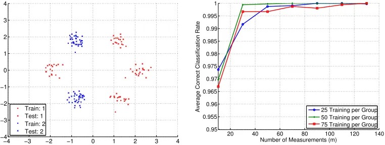
Next, we present a suite of experiments where we again construct the classes as Gaussian

clouds inR2, but utilize various types of data geometries. In each case, we set the number

of training data points for each class to be 25, 50, and 75. In Figure 2, we have two classes forming a total of six Gaussian clouds, and execute Algorithms 1 and 2 using four levels and

m ∈ {10,30,50,70,90,110,130}. The classification accuracy increases for larger m, with

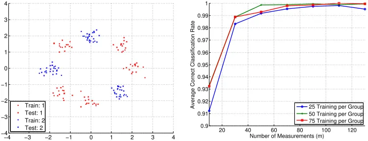
nearly perfect classification for the largest values of m selected. A similar experiment is

shown in Figure 3, where we have two classes forming a total of eight Gaussian clouds, and execute the proposed algorithm using five levels.

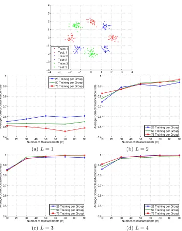
In the next two experiments, we display the classification results of Algorithms 1 and 2

when using m∈ {10,30,50,70,90} and one through four levels, and see that adding levels

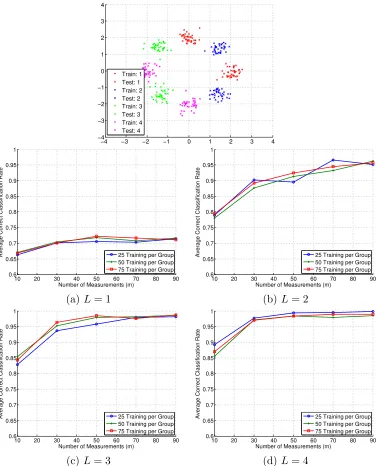
can be beneficial for more complicated data geometries. In Figure 4, we have three classes

(9)

−10 −5 0 5 10 −10

−8 −6 −4 −2 0 2 4 6 8 10

Train: 1

Test: 1 Train: 2 Test: 2

Train: 3 Test: 3

5 10 15 20

0.95 0.955 0.96 0.965 0.97 0.975 0.98 0.985 0.99 0.995 1

Number of Measurements (m)

Average Correct Classification Rate 25 Training per Group 50 Training per Group 75 Training per Group

Figure 1: Synthetic classification experiment with three Gaussian clouds (G= 3), L = 1,

n = 2, 50 test points per group, and 30 trials of randomly generatingA. (Left) Example

training and testing data setup. (Right) Average correct classification rate versus m and

for the indicated number of training points per class.

−4 −3 −2 −1 0 1 2 3 4 −4

−3 −2 −1 0 1 2 3 4

Train: 1 Test: 1 Train: 2

Test: 2 0.95 ₂₀ ₄₀ ₆₀ ₈₀ ₁₀₀ ₁₂₀ ₁₄₀

0.955 0.96 0.965 0.97 0.975 0.98 0.985 0.99 0.995 1

Figure 2: Synthetic classification experiment with six Gaussian clouds and two classes

(G = 2), L = 4, n= 2, 50 test points per group, and 30 trials of randomly generating A.

(Left) Example training and testing data setup. (Right) Average correct classification rate

(10)

toL = 3, there are huge gains in classification accuracy. In Figure 5, we have four classes

forming a total of eight Gaussian clouds. Again, from both L = 1 to L = 2 and L = 2

toL= 3 we see large improvements in classification accuracy, yet still better classification

withL= 4. We note here that in this case it also appears that more training data does not

improve the performance (and perhaps even slightly decreases accuracy); this is of course unexpected in practice, but we believe this happens here only because of the construction of the Gaussian clouds—more training data leads to more outliers in each cloud, making the sets harder to separate.

−4 −3 −2 −1 0 1 2 3 4 −4

−3 −2 −1 0 1 2 3 4

Train: 1 Test: 1 Train: 2 Test: 2

20 40 60 80 100 120

0.9 0.91 0.92 0.93 0.94 0.95 0.96 0.97 0.98 0.99 1

Figure 3: Synthetic classification experiment with eight Gaussian clouds and two classes

(G = 2), L = 5, n= 2, 50 test points per group, and 30 trials of randomly generating A.

(Left) Example training and testing data setup. (Right) Average correct classification rate

versusm and for the indicated number of training points per class.

3.2. Handwritten Digit Classification

In this section, we apply Algorithms 1 and 2 to the MNIST (LeCun, 2018) dataset, which

is a benchmark dataset of images of handwritten digits, each with 28×28 pixels. In total,

the dataset has 60,000 training examples and 10,000 testing examples.

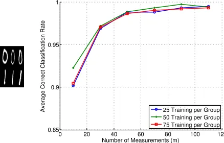
First, we apply Algorithms 1 and 2 when considering only two digit classes.

Fig-ure 6 shows the correct classification rate for the digits “0” versus “1”. We set m ∈

{10,30,50,70,90,110}, p ∈ {50,100,150} with equally sized training data sets for each class, and classify 50 images per digit class. Notice that the algorithm is performing very

well for smallmin comparison ton= 28×28 = 784 and only a single level. Figure 7 shows

the results of a similar setup for the digits “0” and “5”. In this experiment, we increased

to four levels and achieve classification accuracy around 90% at the high end of m values

tested. This indicates that the digits “0” and “5” are more likely to be mixed up than “0” and “1”, which is understandable due to the more similar digit shape between “0” and “5”.

In Figure 7, we include the classification performance when the matrix A is constructed

using the two-dimensional Discrete Cosine Transform (DCT) in addition to our typical

Gaussian matrixA (note one could similarly use the Discrete Fourier Transform instead of

the DCT but that requires re-defining the sign function on complex values). Specifically, to

(11)

−4 −3 −2 −1 0 1 2 3 4 −4

−3 −2 −1 0 1 2 3 4

Train: 1 Test: 1 Train: 2 Test: 2 Train: 3 Test: 3

10 20 30 40 50 60 70 80 90

0.4 0.5 0.6 0.7 0.8 0.9 1

Average Correct Classification Rate

25 Training per Group 50 Training per Group 75 Training per Group

10 20 30 40 50 60 70 80 90

0.4 0.5 0.6 0.7 0.8 0.9 1

(a)L= 1 (b)L= 2

10 20 30 40 50 60 70 80 90

0.4 0.5 0.6 0.7 0.8 0.9 1

10 20 30 40 50 60 70 80 90

0.4 0.5 0.6 0.7 0.8 0.9 1

(c) L= 3 (d)L= 4

Figure 4: Synthetic classification experiment with eight Gaussian clouds and three classes

(G= 3),L= 1, . . . ,4,n= 2, 50 test points per group, and 30 trials of randomly generating

A. (Top) Example training and testing data setup. Average correct classification rate

versusmand for the indicated number of training points per class for: (middle left)L= 1,

(12)

−4 −3 −2 −1 0 1 2 3 4 −4

−3 −2 −1 0 1 2 3 4

Train: 1 Test: 1 Train: 2 Test: 2 Train: 3 Test: 3 Train: 4 Test: 4

10 20 30 40 50 60 70 80 90

0.6 0.65 0.7 0.75 0.8 0.85 0.9 0.95 1

10 20 30 40 50 60 70 80 90

0.6 0.65 0.7 0.75 0.8 0.85 0.9 0.95 1

(a) L= 1 (b)L= 2

10 20 30 40 50 60 70 80 90

0.6 0.65 0.7 0.75 0.8 0.85 0.9 0.95 1

10 20 30 40 50 60 70 80 90

0.6 0.65 0.7 0.75 0.8 0.85 0.9 0.95 1

(c)L= 3 (d)L= 4

Figure 5: Synthetic classification experiment with eight Gaussian clouds and four classes

(G= 4),L= 1, . . . ,4,n= 2, 50 test points per group, and 30 trials of randomly generating

A. (Top) Example training and testing data setup. Average correct classification rate

versusmand for the indicated number of training points per class for: (middle left)L= 1,

(13)

and then apply a random sign (i.e., multiply by +1 or -1) to the columns. We include these two results to illustrate that there is not much difference when using the DCT and Gaussian

constructions ofA, though we expect analyzing the DCT case to be more challenging and

limit the theoretical analysis in this paper to the Gaussian setting. The advantage of using a structured matrix like the DCT is of course the reduction in computation cost in acquiring the measurements.

Training Data

0 20 40 60 80 100 120

0.85 0.9 0.95 1

Testing Data

Figure 6: Classification experiment using the handwritten “0” and “1” digit images from

the MNIST dataset, L= 1, n = 28×28 = 784, 50 test points per group, and 30 trials of

randomly generatingA. (Top left) Training data images whenp= 50. (Top right) Average

correct classification rate versusmand for the indicated number of training points per class.

(Bottom) Testing data images.

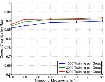
Next, we apply Algorithms 1 and 2 to the MNIST dataset with all ten digits. We

utilize 1,000, 3,000, and 5,000 training points per digit class, and perform

classifica-tion with 800 test images per class. The classificaclassifica-tion results using 18 levels and m ∈

{100,200,400,600,800} are shown in Figure 8, where it can be seen that with 5,000

train-ing points per class, above 90% classification accuracy is achieved form≥200. We also see

that larger training sets result in slightly improved classification.

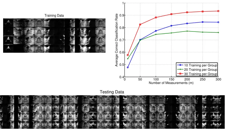
3.3. Facial Recognition

Our last experiment considers facial recognition using the extended YaleB dataset (Cai

et al., 2007b,a, 2006; He et al., 2005). This dataset includes 32×32 images of 38 individuals

with roughly 64 near-frontal images under different illuminations per individual. We select four individuals from the dataset, and randomly select images with different illuminations to be included in the training and testing sets (note that the same illumination was included

foreach individual in the training and testing data). We execute Algorithms 1 and 2 using

(14)

Training Data

Testing Data

20 40 60 80 100

0.6 0.65 0.7 0.75 0.8 0.85 0.9 0.95 1

20 40 60 80 100

0.6 0.65 0.7 0.75 0.8 0.85 0.9 0.95 1

Figure 7: Classification experiment using the handwritten “0” and “5” digit images from

the MNIST dataset, L = 4, n = 28×28 = 784, 50 test points per group, and 30 trials

of randomly generating A. (Top) Training data images when p = 50. (Middle) Testing

data images. Average correct classification rate versus m and for the indicated number of

training points per class (bottom left) when using a Gaussian matrixAand (bottom right)

when using a DCT matrixA.

100 200 300 400 500 600 700 800

0.6 0.65 0.7 0.75 0.8 0.85 0.9 0.95 1

Correct Classification Rate

1000 Training per Group 3000 Training per Group 5000 Training per Group

Figure 8: Correct classification rate versus m when using all ten (0-9) handwritten digits

from the MNIST dataset, L = 18, n = 28×28 = 784, 1,000, 3,000, and 5,000 training

points per group, 800 test points per group (8,000 total), and a single instance of randomly

(15)

in Figure 9. Above 90% correct classification is achieved form≥150 when using the largest training set.

Training Data

0 50 100 150 200 250 300

0.4 0.5 0.6 0.7 0.8 0.9 1

Testing Data

Figure 9: Classification experiment using four individuals from the extended YaleB dataset,

L= 4, n= 32×32 = 1024, 30 test points per group, and 30 trials of randomly generating

A. (Top left) Training data images whenp= 20. (Top right) Average correct classification

rate versusm and for the indicated number of training points per class. (Bottom) Testing

data images.

4. Theoretical Analysis for a Simple Case

4.1. Main Results

We now provide a theoretical analysis of Algorithms 1 and 2 in which we make a series of simplifying assumptions to make the development more tractable. We focus on the setting where the signals are two-dimensional, belonging to one of two classes, and consider a single

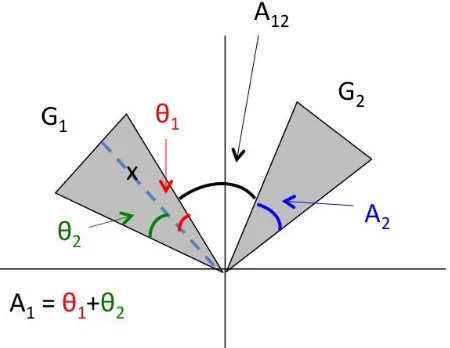
level (i.e., ` = 1, n = 2, and G = 2). Moreover, we assume the true classes G1 and G2

to be two disjoint cones in R2 and assume that regions of the same angular measure have

the same number (or density) of training points. Of course, the problem of non-uniform densities relates to complicated geometries that may dictate the number of training points required for accurate classification (especially when many levels are needed) and is a great direction for future work. However, we believe analyzing this simpler setup will provide a foundation for a more generalized analysis in future work.

Let A1 denote the angular measure ofG1, defined by

A1 = max

x1,x2∈G1

(16)

where ∠(x1, x2) denotes the angle between the vectors x1 and x2; define A2 similarly for

G2. Also, define

A12= min

x1∈G1,x2∈G2

∠(x1, x2)

as the angle between classesG1 and G2. Suppose that the test point x ∈G1, and that we

classifyxusingmrandom hyperplanes. For simplicity, we assume that the hyperplanes can

intersect the cones, but only intersectone cone at a time. This means we are imposing the

conditionA12+A1+A2≤π. See Figure 10 for a visualization of the setup for the analysis.

Notice thatA1 is partitioned into two disjoint pieces, θ1 and θ2, where A1 =θ1+θ2. The

anglesθ1 and θ2 are determined by the location of x within G1.

Figure 10: Visualization of the analysis setup for two classes of two dimensions. If a

hyperplane intersects theθ1 region of G1, thenxis not on the same side of the hyperplane

as G2. If a hyperplane intersects the θ2 region of G1, then x is on the same side of the

hyperplane as G2. That is, θ1 and θ2 are determined by the position of x within G1, and

θ1+θ2 =A1.

The membership index parameter (1) is still used; however, now we have angles instead of numbers of training points. That is,

r(`, i, t, g) = _P_GAg|t j=1Aj|t

PG

j=1|Ag|t−Aj|t|

PG

j=1Aj|t

, (2)

where Ag|t=Ag|t(Λ`,i) denotes the angle of the part of class g with the t-th sign pattern

index at the i-th set selection in the `-th level. Throughout, let t?_i denote the sign pattern

index of the test point x with the i-th hyperplane at the first level, ` = 1; i.e. t?_i = t?_Λ

`,i

with the identification Λ`,i ={i}(since`= 1 implies a single hyperplane is used). Letting

bb_x denote the classification label for x after running the proposed algorithm, Theorem 2

(17)

in Theorem 2 we assume the classes G1 and G2 are of the same size (i.e., A1 =A2) and

the test point x lies in the middle of class G1 (i.e., θ1 = θ2). These assumptions are for

convenience and clarity of presentation only (note that (3) is already quite cumbersome), but the proof follows analogously (albeit without easy simplifications) for the general case; for convenience we leave the computations in Table 1 in general form and do not utilize the

assumptionθ1 =θ2 until the end of the proof. We first state a technical result in Theorem

2, and include two corollaries below that illustrate its usefulness.

Theorem 2 Let the classes G1 and G2 be two cones in R2 defined by angular measures

A1 and A2, respectively, and suppose regions of the same angular measure have the same density of training points. Suppose A1 =A2, θ1 =θ2, and A12+A1+A2 ≤π. Then, the probability that a data point x∈G1 gets classified in class G1 by Algorithms 1 and 2 using a single level and a measurement matrix A ∈ _Rm×2 _{with independent standard Gaussian} entries is bounded as follows,

P[bb_x = 1]≥1−

m

X

j=0

m

X

k1,1=0

m

X

k1,2=0

m

X

k2=0

m

X

k=0

j+k1,1+k1,2+k2+k=m, k1,2≥9(j+k1,1)

m j, k1,1, k1,2, k2, k

A12

π

j

A1

2π

k1,1+k1,2

×

A1

π

k2

π−2A1−A12

π

k

. (3)

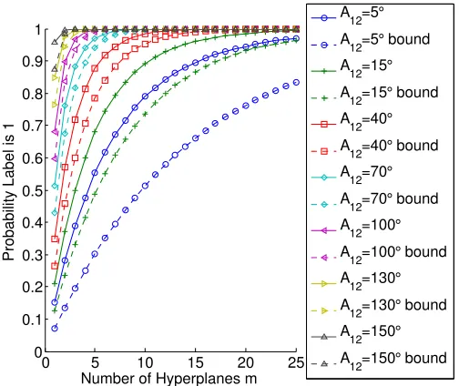
Figure 11 displays the classification probability bound of Theorem 2 compared to the

(sim-ulated) true value of P[bb_x = 1]. Here, A₁ = A₂ = 15◦, θ₁ = θ₂ = 7.5◦, and A₁₂ and m

are varied. Most importantly, notice that in all cases, the classification probability is

ap-proaching 1 with increasing m. Also, the result from Theorem 2 behaves similarly as the

simulated true probability, especially asm and A12 increase.

The following two corollaries provide asymptotic results for situations where P[bb_x = 1]

tends to 1 when m→ ∞. Corollary 3 provides this result whenever A12 is at least as large

as bothA1and π−2A1−A12, and Corollary 4 provides this result for certain combinations

of A1 and A12. These results of course should match intuition, since as m grows large, our

hyperplanes essentially chop up the space into finer and finer wedges. Below, the dependence

on the constants onA1,A12 is explicit in the proofs.

Corollary 3 Consider the setup of Theorem 2. Suppose A12 ≥ A1 and 2A12 ≥π −2A1. Then P[bb_x = 1] → 1 as m → ∞. In fact, the probability converges to 1 exponentially, i.e.

P[ˆbx= 1]≥1−Ce−cm for positive constants c andC that may depend on A1, A12.

Corollary 4 Consider the setup of Theorem 2. SupposeA1+A12>0.58π andA12+3₄A1≤

π

2. Then P[bbx = 1] → 1 as m → ∞. In fact, the probability converges to 1 exponentially, i.e. P[ˆbx= 1]≥1−Ce−cm for positive constants c and C that may depend on A1, A12.

4.2. Proof of Main Results

4.2.1. Proof of Theorem 2

(18)

0 5 10 15 20 25 0

0.1 0.2 0.3 0.4 0.5 0.6 0.7 0.8 0.9 1

Number of Hyperplanes m

Probability Label is 1

A

12=5°

A₁₂=5° bound

A

12=15°

A

12=15° bound

A₁₂=40°

A

12=40° bound

A₁₂=70°

A₁₂=70° bound

A₁₂=100°

A₁₂=100° bound

A

12=130°

A₁₂=130° bound

A

12=150°

A

12=150° bound

Figure 11: P[bb_x = 1] versus the number of hyperplanes m when A₁₂ is varied (see legend),

A1 =A2 = 15◦, and θ1 = θ2 = 7.5◦. The solid lines indicate the probability (5) with the

multinomial probability given by (6) and the conditional probability (9) simulated over 1000 trials of the uniform random variables. The dashed lines indicate the result (3) provided in Theorem 2.

fall on either side of the hyperplane, (ii) the hyperplane completely does not separate the two classes, i.e., the cones fall on the same side of the hyperplane, (iii) the hyperplane cuts

throughG2, (iv) the hyperplane cuts throughG1viaθ1, or (v) the hyperplane cuts through

G1 via θ2. Using this observation, we can now define the event

E(j, k1,1, k1,2, k2) (4)

whereby from among the m total hyperplanes, j hyperplanes separate the cones, k1,1

hy-perplanes cut G1 in θ1, k1,2 hyperplanes cut G1 in θ2, and k2 hyperplanes cut G2. See

Table 1 for an easy reference of these quantities. Note that we must distinguish between

hyperplanes that cut through θ1 and those that cut through θ2; k1,1 hyperplanes cut G1

and land within θ1 so that x isnot on the same side of the hyperplane asG2 whereas k1,2

hyperplanes cutG1 and land within θ2 so that x is on the same side of the hyperplane as

G2. These orientations will affect the computation of the membership index. Using the

above definition of (4), we use the law of total probability to get a handle on P[bb_x = 1], the

probability that the test point x gets classified correctly, as follows,

P[bbx= 1] =P

"_m

X

i=1

r(`, i, t?_i,1)>

m

X

i=1

r(`, i, t?_i,2)

#

= X

j,k1,1,k1,2,k2

j+k1,1+k1,2+k2≤m P

"m

X

i=1

r(`, i, t?i,1)> m

X

i=1

r(`, i, t?i,2)|E(j, k1,1, k1,2, k2)

(19)

×P[E(j, k1,1, k1,2, k2)]. (5)

The latter probability in (5) is similar to the probability density of a multinomial random variable:

P[E(j, k1,1, k1,2, k2)]

=

m

j, k1,1, k1,2, k2, m−j−k1,1−k1,2−k2

A12

π

j

θ1

π

k1,1

θ2

π

k1,2

×

A2

π

k2

π−A1−A2−A12

π

m−j−k1,1−k1,2−k2

, (6)

where _k n

1,k2,...,km

= _k n!

1!k2!···km!.

To evaluate the conditional probability in (5), we must determine the value ofr(`, i, t?_i, g),

for g= 1,2, given the hyperplane cutting pattern event. Table 1 summarizes the possible

cases. In the cases where the hyperplane cuts through either G1 or G2, we model the

location of the hyperplane within the class by a random variable defined on the interval

[0,1], with no assumed distribution. We let u, u0, uh, u0h ∈ [0,1] (for an index h) denote

independent copies of such random variables.

Hyperplane Case Number in event (4) Class g Value ofr(`, i, t?_i, g) (see (2))

(i) separates j 1 1

2 0

(ii) does not separate m−j−k2−k1,1−k1,2

1 A1|A1−A2|

(A1+A2)2

2 A2|A1−A2|

(A1+A2)2

(iii) cutsG2 k2

1 A1|A1−A2u0|

(A1+A2u0)2

2 A2u0|A1−A2u0|

(A1+A2u0)2

(iv) cutsG1,θ1 k1,1

1 1

2 0

(v) cutsG1,θ2 k1,2

1 (θ1+θ2u)|θ1+θ2u−A2|

(θ1+θ2u+A2)2

2 A2|θ1+θ2u−A2|

(θ1+θ2u+A2)2

Table 1: Summary of (2) when up to one cone can be cut per hyperplane, where u, u0 are

independent random variables defined over the interval [0,1].

Using the computations given in Table 1 and assuming j hyperplanes separate (i.e.

condition (i) described above), k1,1 hyperplanes cut G1 in θ1 (condition (iv) above), k1,2

hyperplanes cut G1 in θ2 (condition (v) above), k2 hyperplanes cut G2 (condition (iii)

above), andm−j−k1,1−k1,2−k2 hyperplanes do not separate (condition (ii) above), we

compute the membership index parameters defined in (2) as:

m

X

i=1

r(`, i, t?_i,1) =j+ (m−j−k1,1−k1,2−k2)

A1|A1−A2|

(A1+A2)2

(20)

+ k1,2

X

h=1

(θ1+θ2uh)|θ1+θ2uh−A2|

(θ1+θ2uh+A2)2

+ k2

X

h=1

A1|A1−A2u0_h|

(A1+A2u0_h)2

=j+k1,1+

k1,2

X

h=1

(θ1+θ2uh)|θ1+θ2uh−A1|

(θ1+θ2uh+A1)2

+ k2

X

h=1

A1|A1−A1u0_h|

(A1+A1u0_h)2

(7)

and

m

X

i=1

r(`, i, t?_i,2) = (m−j−k1,1−k1,2−k2)

A2|A1−A2|

(A1+A2)2

+ k1,2

X

h=1

A2|θ1+θ2uh−A2|

(θ1+θ2uh+A2)2

+ k2

X

h=1

A2u0_h|A1−A2u0_h|

(A1+A2u0_h)2

= k1,2

X

h=1

A1|θ1+θ2uh−A1|

(θ1+θ2uh+A1)2

+ k2

X

h=1

A1u0_h|A1−A1u0_h|

(A1+A1u0_h)2

, (8)

where in both cases we have simplified using the assumptionA1=A2. Thus, the conditional

probability in (5), can be expressed as:

P



j+k₁_,₁+

k1,2

X

h=1

|θ1+θ2uh−A1|(θ1+θ2uh−A1)

(θ1+θ2uh+A1)2

+ k2

X

h=1

|A1−A1u0_h|(A1−A1u0_h)

(A1+A1u0_h)2

>0



,

(9)

where it is implied that this probably is conditioned on the hyperplane configuration as in (5). Once the probability (9) is known, we can calculate the full classification probability (5).

Since by assumption,θ1+θ2=A1, we haveθ1+θ2u−A1 ≤0 andA1−A1u0≥0. Thus,

(9) simplifies to

P



j+k1,1−

k1,2

X

h=1

(θ1+θ2uh−A1)2

(θ1+θ2uh+A1)2

+ k2

X

h=1

(A1−A1u0h)2 (A1+A1u0_h)2

>0



 ≥ P[γ > β] (10)

where

β =k1,2

θ2

A1+θ1

2

and γ =j+k1,1.

To obtain the inequality in (10), we used the fact that

j+k1,1−

k1,2

X

h=1

(θ1−A1)2

(θ1+θ2uh+A1)2

+ k2

X

h=1

(A1−A1u0_h)2

(A1+A1u0_h)2

≥j+k1,1−

k1,2

X

h=1

(θ1−A1)2

(θ1+A1)2

+ 0 =γ−β.

By conditioning on γ > β, the probability of interest (5) reduces to (note the bounds on

the summation indices):

P[bb_x= 1] =

X

j,k1,1,k1,2,k2

j+k1,1+k1,2+k2≤m

P

"_m X

i=1

r(`, i, t?_i,1)> m

X

i=1

r(`, i, t?_i,2)|E(j, k1,1, k1,2, k2)

(21)

×_P[E(j, k1,1, k1,2, k2)] (11)

≥ X

j,k1,1,k1,2,k2

j+k1,1+k1,2+k2≤m,

β−γ<0

m

j, k1,1, k1,2, k2, m−j−k1,1−k1,2−k2

A12

π

j

θ1

π

k1,1

×

θ2

π

k1,2

A2

π

k2

π−A1−A2−A12

π

m−j−k1,1−k1,2−k2

. (12)

The condition β −γ < 0 is equivalent to k1,2(_A₁θ₊2_θ₁)2 −(j +k1,1) < 0, which implies

k1,2(_A₁θ₊2_θ₁)2 < j +k1,1. Assuming θ1 = θ2 simplifies this condition to depend only on

the hyperplane configuration (and not A1, θ1, and θ2) since _A₁θ₊2_θ₁ = ₃θ_θ2₂ = 1₃. Thus, the

condition β−γ <0 reduces to the condition k1,2 <9(j+k1,1) and (12) then simplifies to

X

j+k1,1+k1,2+k2≤m,

k1,2<9(j+k1,1)

m

j, k1,1, k1,2, k2, m−j−k1,1−k1,2−k2

A12

π

j

θ1

π

k1,1+k1,2

×

A2

π

k2

π−2A1−A12

π

m−j−k1,1−k1,2−k2

(13)

= X

j+k1,1+k1,2+k2+k=m,

k1,2<9(j+k1,1)

m j, k1,1, k1,2, k2, k

A12

π

j

θ1

π

k1,1+k1,2

A2

π

k2

π−2A1−A12

π

k

,

(14)

= X

j+k1,1+k1,2+k2+k=m,

k1,2<9(j+k1,1)

m j, k1,1, k1,2, k2, k

A12

π

j

A1

2π

k1,1+k1,2

A1

π

k2

π−2A1−A12

π

k

,

(15)

where we have introducedk to denote the number of hyperplanes that do not separate nor

cut through either of the groups, and simplified using the assumptions that θ1 = A₂1 and

A1 =A2.

Note that if we did not have the condition k1,2 < 9(j+k1,1) in the sum (15) (that is,

if we summed over all terms), the quantity would sum to 1 (this can easily be seen by the Multinomial Theorem). Finally, this means (15) is equivalent to (3), thereby completing the proof.

4.2.2. Proof of Corollary 3

Proof We can bound (3) from below by bounding the excluded terms in the sum (i.e.,

those that satisfy k1,2 ≥9(j+k1,1)) from above. One approach to this would be to count

the number of terms satisfyingk1,2 ≥9(j+k1,1) and bound them by their maximum. Using

(22)

k1,2 ≥9(j+k1,1) is given by

W1 =

1 12 jm 10 k + 1 jm 10 k + 2 150 jm 10 k2

−10(4m+ 1)

jm

10

k

+ 3(m2+ 3m+ 2)

∼m4.

(16)

Then, the quantity (3) can be bounded below by

1−W1max

m j, k1,1, k1,2, k2, k

A12

π

j

A1

2π

k1,1+k1,2

A1

π

k2

π−2A1−A12

π

k!

=

1−W1max

m j, k1,1, k1,2, k2, k

1 2

k1,1+k1,2

A12

π

j

A1

π

k1,1+k1,2+k2

π−2A1−A12

π

k!

,

(17)

where the maximum is taken over allj, k1,1, k1,2, k2, k= 0, . . . , msuch thatk1,2≥9(j+k1,1).

Ignoring the constraint k1,2 ≥9(j+k1,1), we can upper bound the multinomial coefficient

using the trivial upper bound of 5m:

m j, k1,1, k1,2, k2, k

≤5m. (18)

Since we are assuming A12 is larger than A1 and π −2A1 −A12 (from the assumption

that 2A12 ≥π−2A1), the strategy is to take j to be as large as possible while satisfying

k1,2 ≥9j and j+k1,2 =m. Since k1,2 ≥9j, we have j+ 9j ≤m which impliesj ≤ m₁₀. So,

we take j= ₁₀m,k1,2= 9₁₀m, and k1,1 =k2 =k= 0. Then

1 2

k1,1+k1,2

A12

π

j

A1

π

k1,1+k1,2+k2

π−2A1−A12

π k (19) ≤ 1 2

9m/10

A12

π

m/10

A1

π

9m/10

= 1 29 A12 π A1 π

9!m/10

. (20)

Combining (17) with the bounds given in (18) and (20), we have

≥1−W15m

1 29 A12 π A1 π

9!m/10

∼1−m45m 1 29 A12 π A1 π

9!m/10

= 1−m2 510 1

29 A12 π A1 π

9!m/10

(23)

For the above to tend to 1 as m → ∞, we need 5₂109 A12 π A1 π 9

< 1. This is equivalent

to A12 A₂1

9

< π₅1010, which implies A12θ91 < π5

10

= π₅ π₅9

. Note that if θ1 = π₅, then

A1 = A2 = 2θ1 = 2₅π. Then A12 could be at most π₅. But, this can’t be because we

have assumed A12 ≥ A1. Thus, we must have θ1 < π₅. In fact, θ1 = π₆ is the largest

possible, in which case A12 = A1 = A2 = π₃. If θ1 = π₆, then A12θ91 < π5

π

5

9

becomes A12 < π₅ 6₅

9

≈ 3.24. Therefore, since we are already assuming A12+ 2A1 ≤ π, this is

essentially no further restriction on A12, and the same would be true for all θ1 ≤ π₆. This

completes the proof.

4.2.3. Proof of Corollary 4

Proof Consider (3) and setj0 =j+k1,1 andr=k2+k. Then we view (3) as a probability

equivalent to

1−

2m

X

j0₌₀

m

X

k1,2=0

2m

X

r=0

j0₊_k

1,2+r=m, k1,2≥9j0

m k1,2, j0, r

_A

12+A₂1

π

!j0

A1

2π

k1,2

π−A1−A12

π

r

. (22)

Note that multinomial coefficients are maximized when the parameters all attain the same

value. Thus, the multinomial term above is maximized when k1,2, j0 and r are all as

close to one another as possible. Thus, given the additional constraint that k1,2 ≥ 9j0,

the multinomial term is maximized when k1,2 = 9₁₉m, j0 = ₁₉m, and r = 9₁₉m (possibly with

ceilings/floors as necessary ifm is not a multiple of 19), (see the appendix, Section A.2, for

a quick explanation), which means

m k1,2, j0, r

≤ m!

(9₁₉m)!(₁₉m)!(9₁₉m)! (23)

∼

√

2πm(m_e)m 2π9₁₉m(9₁₉m_e)18m/19p

2πm₁₉(₁₉m_e)m/19 (24)

= 19 √ 19 18πm (19 9 )

18/19₁₉1/19

m

≈ 19 √

19 18πm2.37

m_, ₍₂₅₎

where (24) follows from Stirling’s approximation for the factorial (and we use the notation

∼to denote asymptotic equivalence, i.e. that two quantities have a ratio that tends to 1 as

the parameter size grows).

Now assume A12+ 3₄A1 ≤ π₂, which implies π−A1−A12 ≥A12+ A₂1. Note also that

π−A1−A12 ≥A1 since it is assumed that π−2A1 −A12 ≥0. Therefore, we can lower

bound (22) by

1−W2

19√19

18πm2.37 m

π−A1−A12

π

m

(24)

whereW2 is the number of terms in the summation in (22), and is given by

W2=

1 6

jm

10

k

+ 1

100jm

10

k2

+ (5−30m)jm

10

k

+ 3(m2+ 3m+ 2)

∼m3. (27)

Thus, (26) goes to 1 asm→ ∞when 2.37 π−A1−A12

π

<1, which holds ifA1+A12>0.58π.

5. Discussion and Conclusion

In this work, we have presented a supervised classification algorithm that operates on binary, or one-bit, data. Along with encouraging numerical experiments, we have also included a theoretical analysis for a simple case. We believe our framework and analysis approach is relevant to analyzing similar, multi-level-type algorithms. Future directions of this work include the use of dithers for more complicated data geometries, identifying settings where real-valued measurements may be worth the additional complexity, analyzing geometries with non-uniform densities of data, as well as a generalized theory for high dimensional data belonging to many classes and utilizing multiple levels within the algorithm. In addition, we believe the framework will extend nicely into other applications such as hierarchical clustering and classification as well as detection problems. In particular, the membership function scores themselves can provide information about the classes and/or data points that can then be utilized for detection, structured classification, false negative rates, and so on. We believe this framework will naturally extend to these types of settings and provide both simplistic algorithmic approaches as well as the ability for mathematical rigor.

Acknowledgments

(25)

Appendix A. Elementary Computations

A.1. Derivation of (16)

Suppose we haveM objects that must be divided into 5 boxes (for us, the boxes are the 5

different types of hyperplanes). Letni denote the number of objects put into boxi. Recall

that in general, M objects can be divided intokboxes M_k+₋₁k−1

ways.

How many arrangements satisfy n1 ≥ 9(n2+n3)? To simplify, let n denote the total

number of objects in boxes 2 and 3 (that is, n =n2 +n3). Then, we want to know how

many arrangements satisfyn1 ≥9n?

If n = 0, then n1 ≥ 9n is satisfied no matter how many objects are in box 1. So, this

reduces to the number of ways to arrangeM objects into 3 boxes, which is given by M₂+2.

Suppose n= 1. For n1 ≥ 9n to be true, we must at least reserve 9 objects in box 1.

ThenM−10 objects remain to be placed in 3 boxes, which can be done in (M−10)+2₂

ways.

But, there are 2 ways for n = 1, eithern2 = 1 or n3 = 1, so we must multiply this by 2.

Thus, (M−10)+2₂ ×2 arrangements satisfyn1 ≥9n.

Continuing in this way, in general for a given n, there are M−10₂n+2×(n+ 1)

arrange-ments that satisfy n1 ≥9n. There aren+ 1 ways to arrange the objects in boxes 2 and 3,

and M−10₂n+2

ways to arrange the remaining objects after 9nhave been reserved in box 1.

Therefore, the total number of arrangements that satisfy n1≥9nis given by

bM

10c

X

n=0

M−10n+ 2

2

×(n+ 1). (28)

To see the upper limit of the sum above, note that we must haveM −10n+ 2≥2, which

means n≤ M₁₀. Since n must be an integer, we take n≤ bM₁₀c. After some heavy algebra

(i.e. using software!), one can express this sum as:

W = 1

12

M 10

+ 1 M

10

+ 2

150

M 10

2

−10(4M+ 1)

M 10

+ 3(M2+ 3M+ 2)

!

(29)

∼M4. (30)

A.2. Derivation of (23)

Suppose we want to maximize (over the choices of a, b, c) a trinomial _am_!_b_!!_c_! subject to a+

b+c = m and a > 9b. Since m is fixed, this is equivalent to choosing a, b, c so as to

minimize a!b!c! subject to these constraints. First, fix c and consider optimizing a and b

subject to a+b = m−c =: k and a > 9b in order to minimize a!b!. For convenience,

suppose k is a multiple of 10. We claim the optimal choice is to set a = 9b (i.e. a= ₁₀9k

and b = ₁₀1 k). Write a = 9b+x where x must be some non-negative integer in order to

satisfy the constraint. We then wish to compare (9b)!b! to (9b+x)!(b−x)!, since the sum

of aand bmust be fixed. One readily observes that:

(9b+x)!(b−x)! = (9b+x)(9b+x−1)· · ·(9b+ 1)

b(b−1)· · ·(b−x+ 1) ·(9b)!b!≥

9b·9b· · ·9b

b·b· · ·b ·(9b)!b! = 9

(26)

Thus, we only increase the producta!b! whena >9b, so the optimal choice is whena= 9b.

This holds for any choice of c. A similar argument shows that optimizingb and c subject

to 9b+b+c = m to minimize (9b)!b!c! results in the choice that c = 9b. Therefore, one

desires thata=c= 9band a+b+c=m, which means a=c= ₁₉9 m andb= ₁₉1 m.

References

Dimitris Achlioptas. Database-friendly random projections: Johnson-lindenstrauss with

binary coins. J. Comput. Syst. Sci., 66(4):671–687, 2003.

Nir Ailon and Bernard Chazelle. Approximate nearest neighbors and the fast

Johnson-Lindenstrauss transform. InProc. 38th annual ACM Symposium on Theory of computing,

pages 557–563. ACM, 2006.

Pervez M Aziz, Henrik V Sorensen, and J Vn der Spiegel. An overview of sigma-delta

converters. IEEE Signal Proc. Mag., 13(1):61–84, 1996.

Richard Baraniuk, Mark Davenport, Ronald DeVore, and Michael Wakin. The

Johnson-Lindenstrauss lemma meets compressed sensing. preprint, 2006.

Richard Baraniuk, Simon Foucart, Deanna Needell, Yaniv Plan, and Mary Wootters.

Expo-nential decay of reconstruction error from binary measurements of sparse signals. IEEE

Trans. Info. Theory, 63(6):3368–3385, 2017.

Petros Boufounos and Richard Baraniuk. 1-bit compressive sensing. InProc. IEEE Conf.

Inform. Science and Systems (CISS), Princeton, NJ, March 2008.

Peter S. Burge, Max R. van Daalen, Barry J. P. Rising, and John S. Shawe-Taylor. Pulsed

neural networks. In Stochastic Bit-stream Neural Networks, pages 337–352. MIT Press,

Cambridge, MA, 1999.

Deng Cai, Xiaofei He, Jiawei Han, and Hong-Jiang Zhang. Orthogonal Laplacianfaces for

face recognition. IEEE Trans. Image Proc., 15(11):3608–3614, 2006.

Deng Cai, Xiaofei He, and Jiawei Han. Spectral regression for efficient regularized subspace

learning. In Proc. Int. Conf. Computer Vision (ICCV’07), 2007a.

Deng Cai, Xiaofei He, Yuxiao Hu, Jiawei Han, and Thomas Huang. Learning a spatially

smooth subspace for face recognition. InProc. IEEE Conf. Computer Vision and Pattern

Recognition Machine Learning (CVPR’07), 2007b.

Robert Calderbank, Sina Jafarpour, and Robert Schapire. Compressed learning: Universal

sparse dimensionality reduction and learning in the measurement domain. preprint, 2009.

Valerio Cambareri, Chunlei Xu, and Laurent Jacques. The rare eclipse problem on tiles:

Quantised embeddings of disjoint convex sets. arXiv preprint arXiv:1702.04664, 2017.

Emmanuel Cand`es, Justin Romberg, and Terrence Tao. Robust uncertainty principles:

Exact signal reconstruction from highly incomplete frequency information. IEEE Trans.

(27)

Emmanuel Cand`es, Justin Romberg, and Terrence Tao. Stable signal recovery from

incom-plete and inaccurate measurements. Comm. Pure Appl. Math., 59(8):1207–1223, 2006b.

James C Candy and Gabor C Temes. Oversampling delta-sigma data converters: theory,

design, and simulation. University of Texas Press, 1962.

Anna Choromanska, Krzysztof Choromanski, Mariusz Bojarski, Tony Jebara, Sanjiv

Ku-mar, and Yann LeCun. Binary embeddings with structured hashed projections. In Proc.

33rd International Conference on Machine Learning, pages 344–353, 2016.

Nello Christianini and John Shawe-Taylor. An Introduction to Support Vector Machines

and Other Kernel-Based Learning Methods. Cambridge University Press, Cambridge, England, 2000.

Matthieu Courbariaux, Yoshua Bengio, and Jean-Pierre David. Binaryconnect: Training

deep neural networks with binary weights during propagations. In Advances in neural

information processing systems, pages 3123–3131, 2015.

Matthieu Courbariaux, Itay Hubara, Daniel Soudry, Ran El-Yaniv, and Yoshua Bengio. Binarized neural networks: Training deep neural networks with weights and activations

constrained to+ 1 or-1. arXiv preprint arXiv:1602.02830, 2016.

Sanjoy Dasgupta and Anupam Gupta. An elementary proof of a theorem of johnson and

lindenstrauss. Random Structures & Algorithms, 22(1):60–65, 2003.

Mark A Davenport, Petros T Boufounos, Michael B Wakin, and Richard G Baraniuk. Signal

processing with compressive measurements. IEEE J. Sel. Topics Signal Process., 4(2):

445–460, 2010.

Sjoerd Dirksen and Alexander Stollenwerk. Fast binary embeddings with gaussian circulant

matrices: improved bounds. arXiv preprint arXiv:1608.06498, 2016.

D. Donoho. Compressed sensing. IEEE Trans. Inform. Theory, 52(4):1289–1306, 2006.

Jun Fang, Yanning Shen, Hongbin Li, and Zhi Ren. Sparse signal recovery from one-bit

quantized data: An iterative reweighted algorithm. Signal Processing, 102:201–206, 2014.

Raja Giryes, Guillermo Sapiro, and Alexander M Bronstein. Deep neural networks with

ran-dom gaussian weights: a universal classification strategy? IEEE Trans. Signal Process.,

64(13):3444–3457, 2016.

Yunchao Gong, Svetlana Lazebnik, Albert Gordo, and Florent Perronnin. Iterative quanti-zation: A procrustean approach to learning binary codes for large-scale image retrieval.

IEEE Trans. Pattern Anal. Machine Intell., 35(12):2916–2929, 2013.

Sivakant Gopi, Praneeth Netrapalli, Prateek Jain, and Aditya V Nori. One-bit compressed

sensing: Provable support and vector recovery. InICML (3), pages 154–162, 2013.

Ankit Gupta, Robert Nowak, and Benjamin Recht. Sample complexity for 1-bit compressed

sensing and sparse classification. InProc. IEEE Int. Symp. Inform. Theory (ISIT), pages

(28)

Jurgen Hahn, Simon Rosenkranz, and Abdelhak M Zoubir. Adaptive compressed

classifi-cation for hyperspectral imagery. In Proc. IEEE Int. Conf. Acoust., Speech, and Signal

Processing (ICASSP), pages 1020–1024. IEEE, 2014.

Xiaofei He, Shuicheng Yan, Yuxiao Hu, Partha Niyogi, and Hong-Jiang Zhang. Face

recog-nition using Laplacianfaces. IEEE Trans. Pattern Anal. Machine Intell., 27(3):328–340,

2005.

Marti A. Hearst, Susan T Dumais, Edgar Osuna, John Platt, and Bernhard Scholkopf.

Support vector machines. IEEE Intelligent Syst. Appl., 13(4):18–28, 1998.

Itay Hubara, Matthieu Courbariaux, Daniel Soudry, Ran El-Yaniv, and Yoshua Bengio. Quantized neural networks: Training neural networks with low precision weights and

activations. arXiv preprint arXiv:1609.07061, 2016.

Blake Hunter, Thomas Strohmer, Theodore E Simos, George Psihoyios, and Ch Tsitouras.

Compressive spectral clustering. In AIP Conference Proceedings, volume 1281, pages

1720–1722. AIP, 2010.

Laurent Jacques, K´evin Degraux, and Christophe De Vleeschouwer. Quantized iterative

hard thresholding: Bridging 1-bit and high-resolution quantized compressed sensing.

arXiv preprint arXiv:1305.1786, 2013a.

Laurent Jacques, Jason Laska, Petros Boufounos, and Richard Baraniuk. Robust 1-bit

compressive sensing via binary stable embeddings of sparse vectors. IEEE Trans. Inform.

Theory, 59(4):2082–2102, 2013b.

Thorsten Joachims. Text categorization with support vector machines: Learning with many

relevant features. Machine learning: ECML-98, pages 137–142, 1998.

William B Johnson and Joram Lindenstrauss. Extensions of Lipschitz mappings into a

Hilbert space. In Proc. Conf. Modern Anal. and Prob., New Haven, CT, June 1982.

Minje Kim and Paris Smaragdis. Bitwise neural networks.arXiv preprint arXiv:1601.06071,

2016.

Felix Krahmer and Rachel Ward. New and improved Johnson–Lindenstrauss embeddings

via the restricted isometry property. SIAM J. Math. Anal., 43(3):1269–1281, 2011.

Alex Krizhevsky, Ilya Sutskever, and Geoffrey E Hinton. Imagenet classification with deep

convolutional neural networks. InProc. Adv. in Neural Processing Systems (NIPS), pages

1097–1105, 2012.

Jason N Laska, Zaiwen Wen, Wotao Yin, and Richard G Baraniuk. Trust, but verify: Fast

and accurate signal recovery from 1-bit compressive measurements. IEEE Trans. Signal

Processing, 59(11):5289–5301, 2011.

Yann LeCun. The MNIST database of handwritten digits, 2018. http://yann.lecun.com/

(29)

Zhouhan Lin, Matthieu Courbariaux, Roland Memisevic, and Yoshua Bengio. Neural

net-works with few multiplications. arXiv preprint arXiv:1510.03009, 2015.

Michele Marchesi, Gianni Orlandi, Francesco Piazza, and Aurelio Uncini. Fast neural

net-works without multipliers. IEEE Trans. Neural Networks, 4(1):53–62, 1993.

Mustafa Ozuysal, Michael Calonder, Vincent Lepetit, and Pascal Fua. Fast keypoint

recog-nition using random ferns. IEEE Trans. Pattern Anal. Machine Intell., 32(3):448–461,

2010.

Yaniv Plan and Roman Vershynin. One-bit compressed sensing by linear programming.

Commun. Pur. Appl. Math., 66(8):1275–1297, 2013a.

Yaniv Plan and Roman Vershynin. Robust 1-bit compressed sensing and sparse logistic

regression: A convex programming approach. IEEE Trans. Inform. Theory, 59(1):482–

494, 2013b.

Yaniv Plan and Roman Vershynin. Dimension reduction by random hyperplane tessellations.

Discrete & Computational Geometry, 51(2):438–461, 2014.

Ali Rahimi and Benjamin Recht. Weighted sums of random kitchen sinks: Replacing

min-imization with randomization in learning. In Proc. Adv. in Neural Processing Systems

(NIPS), pages 1313–1320, 2009.

Mohammad Rastegari, Vicente Ordonez, Joseph Redmon, and Ali Farhadi. Xnor-net:

Ima-genet classification using binary convolutional neural networks. In European Conference

on Computer Vision, pages 525–542. Springer, 2016.

Olga Russakovsky, Jia Deng, Hao Su, Jonathan Krause, Sanjeev Satheesh, Sean Ma, Zhi-heng Huang, Andrej Karpathy, Aditya Khosla, Michael Bernstein, et al. Imagenet large

scale visual recognition challenge. Int. J. Computer Vision, 115(3):211–252, 2015.

Patrice Y Simard and Hans Peter Graf. Backpropagation without multiplication. In Proc.

Adv. in Neural Processing Systems (NIPS), pages 232–239, 1994.

Karen Simonyan and Andrew Zisserman. Very deep convolutional networks for large-scale

image recognition. arXiv preprint arXiv:1409.1556, 2014.

Ingo Steinwart and Andreas Christmann. Support vector machines. Springer Science &

Business Media, 2008.

Christian Szegedy, Wei Liu, Yangqing Jia, Pierre Sermanet, Scott Reed, Dragomir Anguelov, Dumitru Erhan, Vincent Vanhoucke, and Andrew Rabinovich. Going deeper

with convolutions. InProc. IEEE Conf. Computer Vision and Pattern Recognition, pages

1–9, 2015.

Ming Yan, Yi Yang, and Stanley Osher. Robust 1-bit compressive sensing using adaptive

outlier pursuit. IEEE Trans. Signal Processing, 60(7):3868–3875, 2012.

Xinyang Yi, Constantine Caravans, and Eric Price. Binary embedding: Fundamental limits

(30)

Felix X. Yu, Sanjiv Kumar, Yunchao Gong, and Shih-Fu Chang. Circulant binary