Learning from Partial Labels

Learning from Partial Labels

Timothee Cour [email protected]

NEC Laboratories America 10080 N Wolfe Rd # Sw3350 Cupertino, CA 95014, USA

Benjamin Sapp [email protected]

Ben Taskar [email protected]

Department of Computer and Information Science University of Pennsylvania

3330 Walnut Street

Philadelphia, PA 19107, USA

Editor: Yoav Freund

Abstract

We address the problem of partially-labeled multiclass classification, where instead of a single la-bel per instance, the algorithm is given a candidate set of lala-bels, only one of which is correct. Our setting is motivated by a common scenario in many image and video collections, where only partial access to labels is available. The goal is to learn a classifier that can disambiguate the partially-labeled training instances, and generalize to unseen data. We define an intuitive property of the data distribution that sharply characterizes the ability to learn in this setting and show that effec-tive learning is possible even when all the data is only partially labeled. Exploiting this property of the data, we propose a convex learning formulation based on minimization of a loss function appropriate for the partial label setting. We analyze the conditions under which our loss function is asymptotically consistent, as well as its generalization and transductive performance. We apply our framework to identifying faces culled from web news sources and to naming characters in TV series and movies; in particular, we annotated and experimented on a very large video data set and achieve 6% error for character naming on 16 episodes of the TV series Lost.

Keywords: weakly supervised learning, multiclass classification, convex learning, generalization

bounds, names and faces

1. Introduction

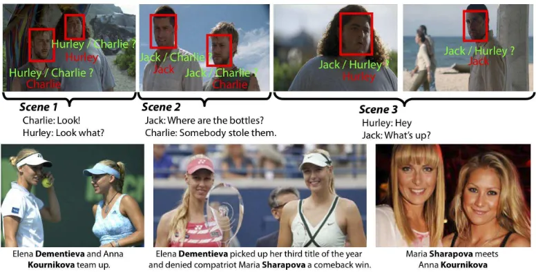
Figure 1: Two examples of partial labeling scenarios for naming faces. Top: using a screenplay, we can tell who is in a movie scene, but for every face in the corresponding images, the person’s identity is ambiguous (green labels). Bottom: images in photograph collections and webpages are often tagged ambiguously with several potential names in the caption or nearby text. In both cases, our goal is to learn a model from ambiguously labeled ex-amples so as to disambiguate the training labels and also generalize to unseen exex-amples.

identity is ambiguous: each face is partially labeled with the set of characters appearing at some point in the scene (Satoh et al., 1999; Everingham et al., 2006; Ramanan et al., 2007). The goal in each case is to learn a person classifier that can not only disambiguate the labels of the training faces, but also generalize to unseen data. Learning accurate models for face and object recognition from such imprecisely annotated images and videos can improve the performance of many applications, including image retrieval and video summarization.

This partially labeled setting is situated between fully supervised and fully unsupervised learn-ing, but is qualitatively different from the semi-supervised setting where both labeled and unlabeled data are available. There have been several papers that addressed this partially labeled (also called ambiguously labeled) problem. Many formulations use the expectation-maximization-like algo-rithms to estimate the model parameters and “fill-in” the labels (Cˆome et al., 2008; Ambroise et al., 2001; Vannoorenberghe and Smets, 2005; Jin and Ghahramani, 2002). Most methods involve ei-ther non-convex objectives or procedural, iterative reassignment schemes which come without any guarantees of achieving global optima of the objective or classification accuracy. To the best of our knowledge, there has not been theoretical analysis of conditions under which proposed approaches are guaranteed to learn accurate classifiers. The contributions of this paper are:

• We show theoretically that effective learning is possible under reasonable distributional as-sumptions even when all the data is partially labeled, leading to useful upper and lower bounds on the true error.

• We apply our convex learning formulation to the task of identifying faces culled from web news sources, and to naming characters in TV series. We experiment on a large data set consisting of 100 hours of video, and in particular achieve 6% (resp. 13%) error for character naming across 8 (resp. 32) labels on 16 episodes of Lost, consistently outperforming several strong baselines.

• We contribute the Annotated Faces on TV data set, which contains about 3,000 cropped faces extracted from 8 episodes of the TV show Lost (one face per track). Each face is registered and annotated with a groundtruth label (there are 40 different characters). We also include a subset of those faces with the partial label set automatically extracted from the screenplay.

• We provide the Convex Learning from Partial Labels Toolbox, an open-source matlab and C++ implementation of our approach as well as the baseline approach discussed in the paper. The code includes scripts to illustrate the process on Faces in the Wild Data Set (Huang et al., 2007a) and our Annotated Faces on TV data set.

The paper is organized as follows.1 We review related work and relevant learning scenarios in Section 2. We pose the partially labeled learning problem as minimization of an ambiguous loss in Section 3, and establish upper and lower bounds between the (unobserved) true loss and the (observed) ambiguous loss in terms of a critical distributional property we call ambiguity degree. We propose the novel Convex Learning from Partial Labels (CLPL) formulation in Section 4, and show it offers a tighter approximation to the ambiguous loss, compared to a straightforward formulation. We derive generalization bounds for the inductive setting, and in Section 5 also provide bounds for the transductive setting. In addition, we provide reasonable sufficient conditions that will guarantee a consistent labeling in a simple case. We show how to solve proposed CLPL optimization problems by reducing them to more standard supervised optimization problems in Section 6, and provide several concrete algorithms that can be adapted to our setting, such as support vector machines and boosting. We then proceed to a series of controlled experiments in Section 7, comparing CLPL to several baselines on different data sets. We also apply our framework to a naming task in TV series, where screenplay and closed captions provide ambiguous labels. The code and data used in the paper can be found at:http://www.vision.grasp.upenn.edu/video.

2. Related Work

We review here the related work for learning under several forms of weak supervision, as well concrete applications.

2.1 Weakly Supervised Learning

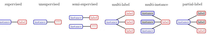
To put the partially-labeled learning problem into perspective, it is useful to lay out several related learning scenarios (see Figure 2), ranging from fully supervised (supervised and multi-label learn-ing), to weakly-supervised (semi-supervised, multi-instance, partially-labeled), to unsupervised.

• In semi-supervised learning (Zhu and Goldberg, 2009; Chapelle et al., 2006), the learner has access to a set of labeled examples as well as a set of unlabeled examples.

supervised

instance label

unsupervised

instance ???

semi-supervised

instance label

instance ???

multi-label

instance label label

label

multi-instance

instance instance

instance

label

partial-label

instance label label

label

Figure 2: Range of supervision in classification. Training may be: supervised (a label is given for each instance), unsupervised (no label is given for any instance), semi-supervised (la-bels are given for some instances), multi-label (each instance can have multiple la(la-bels), multi-instance (a label is given for a group of instances where at least one instance in the group has the label), or partially-labeled (for each instance, several possible labels are given, only one of which is correct).

• In multi-label learning (Boutell et al., 2004; Tsoumakas et al., 2010), each example is as-signed multiple labels, all of which can be true.

• In multi-instance learning (Dietterich et al., 1997; Andrews and Hofmann, 2004; Viola et al., 2006), examples are not individually labeled but grouped into sets which either contain at least one positive example, or only negative examples. A special case considers the easier scenario where label proportions in each bag are known (Kuck and de Freitas, 2005), allowing one to compute convergence bounds on the estimation error of the correct labels (Quadrianto et al., 2009).

• Finally, in our setting of partially labeled learning, also called ambiguously labeled learning, each example again is supplied with multiple labels, only one of which is correct. A formal definition is given in Section 3.

Clearly, these settings can be combined, for example with multi-instance multi-label learning (MIML) (Zhou and Zhang, 2007), where training instances are associated with not only multiple instances but also multiple labels. Another combination of interest appears in a recent paper build-ing on our previous work (Cour et al., 2009) that addresses the case where sets of instances are ambiguously labeled with candidate labeling sets (Luo and Orabona, 2010).

2.2 Learning From Partially-labeled or Ambiguous Data

2.3 Images and Captions

A related multi-class setting is common for images with captions: for example, a photograph of a beach with a palm tree and a boat, where object locations are not specified. Duygulu et al. (2002) and Barnard et al. (2003) show that such partial supervision can be sufficient to learn to identify the object locations. The key observation is that while text and images are separately ambiguous, jointly they complement each other. The text, for instance, does not mention obvious appearance properties, but the frequent co-occurrence of a word with a visual element could be an indication of association between the word and a region in the image. Of course, words in the text without correspondences in the image and parts of the image not described in the text are virtually inevitable. The problem of naming image regions can be posed as translation from one language to another. Barnard et al. (2003) address it using a multi-modal extension to mixture of latent Dirichlet allocations.

2.4 Names and Faces

The specific problem of naming faces in images and videos using text sources has been addressed in several works (Satoh et al., 1999; Berg et al., 2004; Gallagher and Chen, 2007; Everingham et al., 2006). There is a vast literature on fully supervised face recognition, which is out of the scope of this paper. Approaches relevant to ours include Berg et al. (2004), which aims at clustering face images obtained by detecting faces from images with captions. Since the name of the depicted people typically appears in the caption, the resulting set of images is ambiguously labeled if more than one name appears in the caption. Moreover, in some cases the correct name may not be included in the set of potential labels for a face. The problem can be solved by using unambiguous images to estimate discriminant coordinates for the entire data set. The images are clustered in this space and the process is iterated. Gallagher and Chen (2007) address the similar problem of retrieval from consumer photo collections, in which several people appear in each image which is labeled with their names. Instead of estimating a prior probability for each individual, the algorithm estimates a prior for groups using the ambiguous labels. Unlike Berg et al. (2004), the method of Gallagher and Chen (2007) does not handle erroneous names in the captions.

2.5 People in Video

In work on video, a wide range of cues has been used to automatically obtain supervised data, including: captions or transcripts (Everingham et al., 2006; Cour et al., 2008; Laptev et al., 2008), sound (Satoh et al., 1999) to obtain the transcript, or clustering based on clothing, face and hair color within scenes to group instances (Ramanan et al., 2007). Most of the methods involve either procedural, iterative reassignment schemes or non-convex optimization.

3. Formulation

In the standard supervised multiclass setting, we have labeled examples S=_{(xi,yi)mi=1} from an

unknown distribution P(X,Y)where X _∈

X

zi as the ambiguity set actually observed by the learning algorithm, where zi ⊆ {1, . . . ,L} \ {yi}

is a set of additional labels, and yi the latent groundtruth label which we would like to recover.

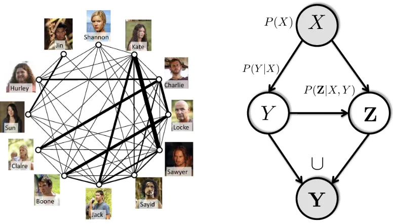
Figure 3: Left: Co-occurrence graph of the top characters across 16 episodes of Lost. Edge thick-ness corresponds to the co-occurrence frequency of characters. Right: The model of the data generation process:(X,Y)are observed,(Y,Z)are hidden, with Y=Y_∪Z.

with corresponding lowercase values of random variables. We suppose X,Y,Z are distributed according to an (unknown) distribution P(X,Y,Z) =P(X)P(Y _|X)P(Z_|X,Y)(see Figure 3, right), of which we only observe samples of the form S=_{(xi,yi)mi=1}={(xi,{yi} ∪zi)mi=1}. (In case X is

continuous, P(X)is a density with respect to some underlying measure µ on

X

Y _∈Y,Z_⊂Y,Y _∈/Z.

Clearly, our setup generalizes the standard semi-supervised setting where some examples are labeled and some are unlabeled: an example is labeled when the corresponding ambiguity set yiis a

singleton, and unlabeled when yiincludes all the labels. However, we do not explicitly consider the

semi-supervised setting this paper, and our analysis below provides essentially vacuous bounds for the semi-supervised case. Instead, we consider the middle-ground, where all examples are partially labeled as described in our motivating examples and analyze assumptions under which learning can be guaranteed to succeed.

In order to learn from ambiguous data, we must make some assumptions about the distribution P(Z|X,Y). Consider a very simple ambiguity pattern that makes accurate learning impossible: L=3,_|zi|=1 and label 1 is present in every set yi, for all i. Then we cannot distinguish between the

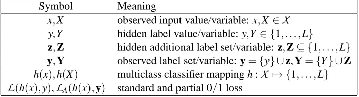
Symbol Meaning

x,X observed input value/variable: x,X_∈

X

y,Y hidden label value/variable: y,Y _{∈ {}1, . . . ,L_}

z,Z hidden additional label set/variable: z,Z⊆ {1, . . . ,L} y,Y observed label set/variable: y=_{y_{} ∪}z,Y=_{Y_{} ∪}Z h(x),h(X) multiclass classifier mapping h :

X

L

L

Table 1: Summary of notation used.

where the thickness of the edges corresponds to the number of times characters share a scene. This suggests that for most characters, ambiguity sets are diverse and we can expect that the ambiguity degree is small. A more quantitative diagram will be given in Figure 11 (left).

Many formulations of fully-supervised multiclass learning have been proposed based on mini-mization of convex upper bounds on risk, usually, the expected 0/1 loss (Zhang, 2004):

0/1 loss:

L

where h(x):

X

We cannot evaluate the 0/1 loss using our partially labeled training data. We define a surro-gate loss which we can evaluate, and we call ambiguous or partial 0/1 loss (where A stands for ambiguous):

Partial 0/1 loss:

L

3.1 Connection Between Partial and Standard 0/1 Losses

An obvious observation is that the partial loss is an underestimate of the true loss. However, in the ambiguous learning setting we would like to minimize the true 0/1 loss, with access only to the partial loss. Therefore we need a way to upper-bound the 0/1 loss using the partial loss. We first introduce a measure of hardness of learning under ambiguous supervision, which we define as ambiguity degreeεof a distribution P(X,Y,Z):

Ambiguity degree: ε= sup

x,y,z:P(x,y)>0,z∈{1,...,L}

P(z_∈Z_|X=x,Y=y). (1)

In words, ε corresponds to the maximum probability of an extra label z co-occurring with a true label y, over all labels and inputs. Let us consider several extreme cases: Whenε=0, Z= /0

with probability one, and we are back to the standard supervised learning case, with no ambiguity. Whenε=1, some extra label always co-occurs with a true label y on an example x and we cannot tell them apart: no learning is possible for this example. For a fixed ambiguity set size C (i.e., P(_|Z_|=C) =1), the smallest possible ambiguity degree is ε=C/(L₋1), achieved for the case where P(Z_|X,Y)is uniform over subsets of size C, for which we have P(z_∈Z_|X,Y) =C/(L₋1)

for all z_{∈ {}1, . . . ,L_}\{y_}. Intuitively, the best case scenario for ambiguous learning corresponds to a distribution with high conditional entropy for P(Z_|X,Y).

Proposition 1 (Partial loss bound via ambiguity degreeε) For any classifier h and distribution P(X,Y,Z), with Y=X_∪Z and ambiguity degreeε:

EP[

L

L

1

1₋εEP[

L

with the convention 1/0= +∞. These bounds are tight, and for the second one, for any (rational)

ε, we can find a number of labels L, a distribution P and classifier h such that equality holds.

Proof. All proofs appear in Appendix B.

3.2 Robustness to Outliers

One potential issue with Proposition 1 is that unlikely (outlier) pairs x,y (with vanishing P(x,y)) might forceεto be close to 1, making the bound very loose. We show we can refine the notion of ambiguity degreeεby excluding such pairs.

Definition 2 (ε,δ)-ambiguous distribution. A distribution P(X,Y,Z)is(ε,δ)-ambiguous if there exists a subset G of the support of P(X,Y), G_⊆

X

X

sup

(x,y)∈G,z∈{1,...,L}

P(z_∈Z_|X=x,Y =y)_≤ε.

Note that in the extreme caseε=0 corresponds to standard semi-supervised learning, where 1₋δ-proportion of examples are unambiguously labeled, andδare (potentially) fully unlabeled. Even though we can accommodate it, semi-supervised learning is not our focus in this paper and our bounds are not well suited for this case.

This definition allows us to bound the 0/1 loss even in the case when some unlikely set of pairs x,y with probability_≤δwould make the ambiguity degree large. Suppose we mix an initial distribution with small ambiguity degree, with an outlier distribution with large overall ambiguity degree. The following proposition shows that the bound degrades only by an additive amount, which can be interpreted as a form of robustness to outliers.

Proposition 3 (Partial loss bound via(ε,δ)) For any classifier h and(ε,δ)-ambiguous P(Z_|X,Y),

EP[

L

1

1₋εEP[

L

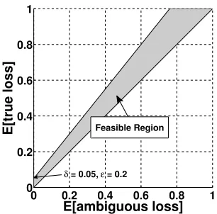
A visualization of the bounds in Proposition 1 and Proposition 3 is shown in Figure 4.

3.3 Label-specific Recall Bounds

0 0.2 0.4 0.6 0.8 1 0

0.2 0.4 0.6 0.8 1

E[ambiguous loss]

E[true loss] Feasible Region

δ = 0.05, ε = 0.2

Figure 4: Feasible region for expected ambiguous and true loss, forε=0.2,δ=0.05.

0/1 loss if we consider label-specific information. We define the label-specific ambiguity degreeεa

of a distribution (with a_{∈ {}1, . . . ,L_}) as:

εa= sup

x,z:P(X=x,Y=a)>0;z∈{1,...,L}

P(z_∈Z_|X=x,Y =a).

We can show a label-specific analog of Proposition 1:

Proposition 4 (Label-specific partial loss bound) For any classifier h and distribution P(X,Y,Z)

with label-specific ambiguity degreeεa,

EP[L(h(X),Y)|Y =a]≤

1 1₋εa

EP[LA(h(X),Y)|Y=a],

where we see thatεabounds per-class recall.

These bounds give a strong connection between ambiguous loss and real loss whenεis small. This assumption allows us to approximately minimize the expected real loss by minimizing (an upper bound on) the ambiguous loss, as we propose in the following section.

4. A Convex Learning Formulation

We have not assumed any specific form for our classifier h(x)above. We now focus on a particular family of classifiers, which assigns a score ga(x)to each label a for a given input x and select the

highest scoring label:

h(x) =arg max

a∈1..Lga(x).

We assume that ties are broken arbitrarily, for example, by selecting the label with smallest index a. We define the vector g(x) = [g1(x). . .gL(x)]⊤, with each component ga:

X

G

G

X

each class, bounded by some norm:_||wa||p≤B for p=1,2.

components of g to create a multiclass loss. For example, we can use hinge, exponential or logistic loss. In particular, we assume a type of one-against-all scheme for the supervised case:

L

∑

a6=y

ψ(₋ga(x)).

A classifier hg(x) is selected by minimizing the empirical loss

L

(called empiricalψ-risk) over the function class

G

inf

g∈GES[

L

1 m

m

∑

i=1

L

For the fully supervised case, under appropriate assumptions, this form of the multiclass loss is infinite-sample consistent. This means that a minimizer ˆg of ψ-risk achieves optimal 0/1 risk infgES[

L

L

that the function class

G

X

differentiable and(4)ψ(u)<ψ(₋u)when u>0 (Theorem 9 in Zhang (2004)). These conditions are satisfied, for example, for the exponential, logistic and squared hinge loss max(0,1₋u)2_{. Below,} we construct a loss function for the partially labeled case and consider when the proposed loss is consistent.

4.1 Convex Loss for Partial Labels

In the partially labeled setting, instead of an unambiguous single label y per instance we have a set of labels Y , one of which is the correct label for the instance. We propose the following loss, which we call our Convex Loss for Partial Labels (CLPL):

L

|y_|a

∑

!

+

∑

a∈/y

ψ(₋ga(x)). (2)

Note that if y is a singleton, the CLPL function reduces to the regular multiclass loss. Otherwise, CLPL will drive up the average of the scores of the labels in y. If the score of the correct label is large enough, the other labels in the set do not need to be positive. This tendency alone does not guarantee that the correct label has the highest score. However, we show in Proposition 6 that

L

L

Of course, minimizing an upperbound on the loss does not always lead to sensible algorithms. We show next that our loss function is consistent under certain assumptions and offers a tighter upperbound to the ambiguous loss compared to a more straightforward multi-label approach.

4.2 Consistency for Partial Labels

We derive conditions under which the minimizer of the CLPL in Equation 2 with partial labels achieves optimal 0/1 risk: infg∈GES[

L

L

may not be unique. First, we require that arg maxaP(Y =a|X=x) =arg maxaP(a∈Y|X =x),

since otherwise arg maxaP(Y=a|X=x)cannot be determined by any algorithm from partial labels

Y without additional information even with an infinite amount of data. Second, we require a simple dominance condition as detailed below and provide a counterexample when this condition does not hold. The dominance relation defined formally below states that when a is the most (or one of the most) likely label given x according to P(Y_|X =x) and b is not, c_{∪ {}a_} has higher (or equal) probability than c_{∪ {}b_}for any set of other labels c.

Proposition 5 (Partial label consistency) Suppose the following conditions hold:

• ψ(_·)is differentiable, convex, lower-bounded and non-increasing, withψ′(0)<0.

• When P(X=x)>0, arg maxa′P(Y =a′|X=x) =arg max_a′P(a′∈Y|X=x).

• The following dominance relation holds:_∀a_∈arg max_a′P(a′∈Y|X=x), ∀b6∈arg max_a′

P(a′_∈Y_|X=x), _∀c_{⊂ {}1, . . . ,L_}\{a,b_}:

P(Y=c_{∪ {}a_{} |}X=x)_≥P(Y=c_{∪ {}b_{} |}X =x).

Then

L

inf

g∈GES[

L

L

as_|S_|=m_→∞and

G

If the dominance relation does not hold, we can find counter-examples where consistency fails. Consider a distribution with a single x with P(x)>0, and let L=4, P(_|Y_|=2_|X =x) =1,ψbe the square-hinge loss, and P(Y_|X=x)be such that:

a 250_·Pab 1 2 3 4

b

1 0 29 44 0

2 29 0 17 26

3 44 17 0 9

4 0 26 9 0

250_·Pa 73 72 70 35

Above, the abbreviations are Pab=P(Y={a,b} |X=x)and Pa=∑bPab, and the entries that do not

satisfy the dominance relation are in bold. We can explicitly compute the minimizer of

L

2Pab+diag(2− 3

2Pa))−1(3Pa−2)≈ −

0.6572 0.6571 0.6736 0.8568 . It satisifes arg max_aga=2 but arg maxa∑bPab=1.

4.3 Comparison to Other Loss Functions

The “naive” partial loss, proposed by Jin and Ghahramani (2002), treats each example as having multiple correct labels, which implies the following loss function

L

square hinge

chord

g

g

naive

ours

max

! "#$ " %#$ % %#$ " "#$ ! %

%#$ " "#$ ! !#$ 3 &#$ 4 '#$ $

ours

max

naive

! "#$ " %#$ % %#$ " "#$ ! %

%#$ " "#$ ! !#$ 3 &#$ 4 '#$

naive

ours

max

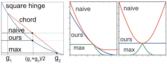
Figure 5: Our loss function in Equation 2 provides a tighter convex upperbound than the naive loss Equation 3 on the non-convex max-loss Equation 4. (Left) We show the square hinge ψ(blue) and a chord (red) touching two points g1,g2. The horizontal lines correspond to our lossψ(1₂(g1+g2))Equation 2, the max-loss ψ(max(g1,g2)), and the naive loss

1

2(ψ(g1) +ψ(g2))(ignoring negative terms and assuming y={1,2}). (Middle) Corre-sponding losses as we vary g1∈[₋2,2](with g2=0). (Right) Same, with g2=₋g1. One reason we expect our loss function to outperform the naive approach is that we obtain a tighter convex upper bound on

L

L

max

a∈y ga(x)

+

∑

a∈/y

ψ(₋ga(x)), (4)

which is not convex, but is in some sense closer to the desired true loss. The following inequalities are verified for common lossesψ such as square hinge loss, exponential loss, and log loss with proper scaling:

Proposition 6 (Comparison between partial losses) Under the usual conditions thatψis a con-vex, decreasing upper bound of the step function, the following inequalities hold:

2

L

L

L

L

The 2ndand 3rdbounds are tight, and the first one is tight providedψ(0) =1 and lim+∞ψ=0.

This shows that our CLPL

L

L

L

Figure 5. To gain additional intuition as to why CLPL is better than the naive loss Equation 3: for an input x with ambiguous label set(a,b), CLPL only encourages the average of ga(x) and gb(x)

to be large, allowing the correct score to be positive and the extraneous score to be negative (e.g., ga(x) =2,gb(x) =−1). In contrast, the naive model encourages both ga(x)and gb(x)to be large.

4.4 Generalization Bounds

We useψ(u) =max(0,1−u)p_{(for example hinge loss with p=1, squared hinge loss with p=2).}

The corresponding margin-based loss is defined via a truncated, rescaled version ofψ:

ψγ(u) =

  

 

1 if u_≤0,

(1₋u/γ)p _{if 0<u≤}γ_,

0 if u>γ.

Proposition 7 (Generalization bound) For any integer m and anyη_∈(0,1), with probability at least 1₋ηover samples S=_{(xi,yi)}mi=1, for every g in

G

EP[

L

L

4pBL5/2 cγ

r

ES[||f(X)||2]

m +L

r

8 log(2/η)

m .

where c is an absolute constant from Lemma 12 in the appendix,ESis the sample average and L is

the number of labels.

The proof in the appendix uses definition 11 for Rademacher and Gaussian complexity, Lemma 12, Theorem 13 and Theorem 14 from Bartlett and Mendelson (2002), reproduced in the appendix and adapted to our notations for completeness. Using Proposition 7 and Proposition 1, we can derive the following bounds on the true expected 0/1 lossEP[

L

Proposition 8 (Generalization bounds on true loss) For any distribution ε-ambiguous distribu-tion P, integer m andη_∈(0,1), with probability at least 1₋ηover samples S=_{(xi,yi)}mi=1, for every g_∈

G

EP[

L

1 1₋ε



_ES[

L

4pBL5/2 cγ

r

ES[||f(X)||2]

m +L

s

8 log2_η m



.

5. Transductive Analysis

We now turn to the analysis of our Convex Loss for Partial Labels (CLPL) in the transductive setting. We show guarantees on disambiguating the labels of instances under fairly reasonable assumptions.

Example 1 Consider a data set S of two points, x,x′, with label sets_{1,2_},_{1,3_}, respectively and suppose that the total number of labels is 3. The objective function is given by:

ψ(1

2(g1(x) +g2(x))) +ψ(−g3(x)) +ψ( 1 2(g1(x

′_{) +g}

3(x′))) +ψ(−g2(x′)).

Suppose the correct labels are(1,1). It is clear that without further assumptions about x and x′ we cannot assume that the minimizer of the loss above will predict the right label. However, if f(x)

and f(x′)are close, it should be intuitively clear that we should be able to deduce the label of the two examples is 1.

5.1 Definitions

In the remainder of this section, we denote y(x) (resp. y(x)) as the true label (resp. ambiguous label set) of some x_∈S, and z(x) =y(x)_\{y(x)_}. _{|| · ||}denotes an arbitrary norm, with_{|| · ||}∗ its dual norm. As above,ψdenotes a decreasing upper bound on the step function and g a classifier satisfying: _∀a, _||wa||∗≤1 (we can easily generalize the remaining propositions to the case where

gais 1-Lipschitz and f is the identity). For x∈S andη>0, we define Bη(x)as the set of neighbors

of x that have the same label as x:

Bη(x) =_{x′_∈S_\{x_}:_||f(x′)₋f(x)_||<η,y(x′) =y(x)_}.

Lemma 9 Let x∈S. If

L

−η/2, then g predicts the correct label for x.

In other words, g predicts the correct label for x when its loss is sufficiently small, and for each of its ambiguous labels a, we can find a neighbor with same label whose score ga(x′)is small enough.

Note that this does not make any assumption on the nearest neighbors of x.

Corollary 10 Let x _∈ S. Suppose _∃q _≥ 0, x1...xq ∈ Bη(x) such that ∩i=0..qz(xi) = /0,

maxi=0..q

L

In other words, g predicts the correct label for x if we can find a set of neighbors of the same label with small enough loss, and without any common extra label. This simple condition often arises in our experiments.

6. Algorithms

Our formulation is quite flexible and we can derive many alternative algorithms depending on the choice of the binary lossψ(u), the regularization, and the optimization method. We can minimize Equation 2 using off-the-shelf binary classification solvers. To do this, we rewrite the two types of terms in Equation 2 as linear combinations of m_·L feature vectors. We stack the parameters and features into one vector as follows below, so that ga(x) =wa·f(x) =w·f(x,a):

w=





w1 . . . wL



; f(x,a) =





1(a=1)f(x)

. . .

1(a=L)f(x)



.

We also define f(x,y)to be the average feature vector of the labels in the set y:

f(x,y) = 1

|y_|a

∑

With these definitions, we have:

L

∑

a∈/y

ψ(₋w_·f(x,a)).

and∑iL− |yi|negative examples S−={f(xi,a)}m_i=1,a∈/yi. Note that the increase in dimension of the

features by a factor of L does not significantly affect the running time of most methods since the vectors are sparse. We use the off-the-shelf implementation of binary SVM with squared hinge (Fan et al., 2008) in most of our experiments, where the objective is:

min

w

1 2||w||

2 2+C

∑

i

max(0,1₋w_·f(xi,yi))2+C

∑

max(0,1+w_·f(xi,a))2.

Using hinge loss and L1regularization lead to a linear programming formulation, and using L1 with exponential loss leads naturally to a boosting algorithm. We present (and experiment with) a boosting variant of the algorithm, allowing efficient feature selection, as described in Appendix A. We can also consider the case where the regularization is L2 and f(x):

X

w=

∑

i

αif(xi,yi)−

∑

αi,af(xi,a),

for some set of non-negative α’s, whereαi corresponds to the positive example f(xi,yi), andαi,a

corresponds to the negative example f(xi,a), for a∈/yi. Letting K(x,x′) =f(x)·f(x′)be the kernel

function, note that f(x,a)_·f(x′,b) =1(a=b)K(x,x′). Hence, we have:

w_·f(x,b) =

∑

i,a∈yi αi

|yi|1

(a=b)K(xi,x)−

∑

αi,a1(a=b)K(xi,x).

This transformation allows us to use kernels with standard off-the-shelf binary SVM implementa-tions.

7. Controlled Partial Labeling Experiments

We first perform a series of controlled experiments to analyze our Convex Learning from Partial La-bels (CLPL) framework on several data sets, including standard benchmarks from the UCI repos-itory (Asuncion and Newman, 2007), a speaker identification task from audio extracted from movies, and a face naming task from Labeled Faces in the Wild (Huang et al., 2007b). In Section 8 we also consider the challenging task of naming characters in TV shows throughout an entire season. In each case the goal is to correctly label faces/speech segments/instances from examples that have multiple potential labels (transductive case), as well as learn a model that can generalize to other unlabeled examples (inductive case).

7.1 Baselines

In the experiments, we compare CLPL with the following baselines.

7.1.1 CHANCEBASELINE

We define the chance baseline as randomly guessing between the possible ambiguous labels only. Defining the (empirical) average ambiguous size to beES[|y|] = _m1∑mi=1|yi|, then the expected error

from the chance baseline is given by errorchance=1_−ES1_[|y|]. 7.1.2 NAIVEMODEL

We report results on an un-normalized version of the naive model introduced in Equation 3: ∑a∈yψ(ga(x)) +∑a∈/yψ(−ga(x)), but both normalized and un-normalized versions produce very

similar results. After training, we predict the label with the highest score (in the transductive set-ting): ˆy=arg maxa_∈yga(x).

7.1.3 IBM MODEL1

This generative model was originally proposed in Brown et al. (1993) for machine translation, but we can adapt it to the ambiguous label case. In our setting, the conditional probability of observ-ing example x_∈Rd given that its label is a is Gaussian: x_∼N(µa,Σa). We use the

expectation-maximization (EM) algorithm to learn the parameters of the Gaussians (mean µa and diagonal

co-variance matrixΣa=diag(σa)for each label).

7.1.4 DISCRIMINATIVEEM

We compare with the model proposed in Jin and Ghahramani (2002), which is a discriminative model with an EM procedure adapted for the ambiguous label setting. The authors minimize the KL divergence between a maximum entropy model P (estimated in the M-step) and a distribution over ambiguous labels ˆP (estimated in the E-step):

J(θ,_Pˆ_{) =}

∑

i a

∑

ˆ

P(a_|xi)log

_ˆ

P(a_|xi)

P(a_|xi,θ)

.

7.1.5 K-NEARESTNEIGHBOR

Following Hullermeier and Beringer (2006), we adapt the k-Nearest Neighbor Classifier to the ambiguous label setting as follows:

knn(x) =arg max

a∈y

k

∑

i=1

wi1(a∈yi), (5)

where xi is the ith nearest-neighbor of x using Euclidean distance, and wi are a set of weights. We

use two kNN baselines: kNN assumes uniform weights wi =1 (model used in Hullermeier and

Beringer, 2006), and weighted kNN uses linearly decreasing weights wi=k−i+1. We use k=5

7.1.6 SUPERVISED MODELS

Finally we also consider two baselines that ignore the ambiguous label setting. The first one, de-noted as supervised model, removes from Equation 3 the examples with_|y_|>1. The second model, denoted as supervised kNN, removes from Equation 5 the same examples.

7.2 Data Sets and Feature Description

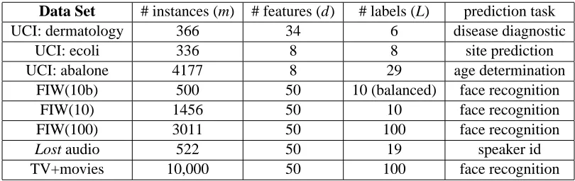
We describe below the different data sets used to report our experiments. The experiments for automatic naming of characters in TV shows can be found in Section 8. A concise summary is given in Table 2.

Data Set # instances (m) # features (d) # labels (L) prediction task

UCI: dermatology 366 34 6 disease diagnostic

UCI: ecoli 336 8 8 site prediction

UCI: abalone 4177 8 29 age determination

FIW(10b) 500 50 10 (balanced) face recognition

FIW(10) 1456 50 10 face recognition

FIW(100) 3011 50 100 face recognition

Lost audio 522 50 19 speaker id

TV+movies 10,000 50 100 face recognition

Table 2: Summary of data sets used in our experiments. The TV+movies experiments are treated in Section 8. Faces in the Wild (1) uses a balanced distribution of labels (first 50 images for the top 10 most frequent people).

7.2.1 UCI DATASETS

We selected three biology related data sets from the publicly available UCI repository (Asuncion and Newman, 2007): dermatology, ecoli, abalone. As a preprocessing step, each feature was inde-pendently scaled to have zero mean and unit variance.

7.2.2 FACES IN THEWILD (FIW)

We experiment with different subsets of the publicly available Labeled Faces in the Wild (Huang et al., 2007a) data set. We use the images registered with funneling (Huang et al., 2007a), and crop out the central part corresponding to the approximate face location, which we resize to 60x90. We project the resulting grayscale patches (treated as 5400x1 vectors) onto a 50-dimensional subspace using PCA.2In Table 2, FIW(10b) extracts the first 50 images for each of the top 10 most frequent people (balanced label distribution); FIW(10) extracts all images for each of the top 10 most fre-quent people (heavily unbalanced label distribution, with 530 hits for George Bush and 53 hits for John Ashcroft); FIW(100) extracts up to 100 faces for each of the top 100 most frequent people (again, heavily unbalanced label distribution).

7.2.3 SPEAKERIDENTIFICATIONFROMAUDIO

We also investigate a speaker identification task based on audio in an uncontrolled environment. The audio is extracted from an episode of Lost (season 1, episode 5) and is initially completely unaligned. Compared to recorded conversation in a controlled environment, this task is more re-alistic and very challenging due to a number of factors: background noise, strong variability in tone of voice due to emotions, and people shouting or talking at the same time. We use the Hid-den Markov Model Toolkit (HTK) (http://htk.eng.cam.ac.uk/) to compute forced alignment (Moreno et al., 1998; Sj¨olander, 2003), between the closed captions and the audio (given the rough initial estimates from closed caption time stamps, which are often overlapping and contain back-ground noise). After alignment, our data set is composed of 522 utterances (each one corresponding to a closed caption line, with aligned audio and speaker id obtained from aligned screenplay), with 19 different speakers. For each speech segment (typically between 1 and 4 seconds) we extract standard voice processing audio features: pitch (Talkin, 1995), Mel-Frequency Cepstral Coefficients (MFCC) (Mermelstein, 1976), Linear predictive coding (LPC) (Proakis and Manolakis, 1996). This results in a total of 4,000 features, which we normalize to the range[₋1,1]and then project onto 50 dimensions using PCA.

7.3 Experimental Setup

For the inductive experiments, we split randomly in half the instances into (1) ambiguously la-beled training set, and (2) unlala-beled testing set. The ambiguous labels in the training set are generated randomly according to different noise models which we specify in each case. For each method and parameter setting, we report the average test error rate over 20 trials after training the model on the ambiguous train set. We also report the corresponding standard deviation as an error bar in the plots. Note, in the inductive setting we consider the test set as unlabeled, thus the classifier votes among all possible labels:

a∗=h(x) =arg max

a∈{1..L}ga(x).

For the transductive experiments, there is no test set; we report the error rate for disambiguating the ambiguous labels (also averaged over 20 trials corresponding to random settings of ambiguous labels). The main differences with the inductive setting are: (1) the model is trained on all instances and tested on the same instances; and (2) the classifier votes only among the ambiguous labels, which is easier:

a∗=h(x) =arg max

a∈y ga(x).

We compare our CLPL approach (denoted as mean in figures, due to the form of the loss) against the baselines presented in Section 7.1: Chance, Model 1, Discriminative EM model, k-Nearest Neighbor, weighted k-k-Nearest Neighbor, Naive model, supervised model, and supervised kNN. Note, in our experiments the Discriminative EM model was much slower to converge than all the other methods, and we only report the first series of experiments with this baseline.

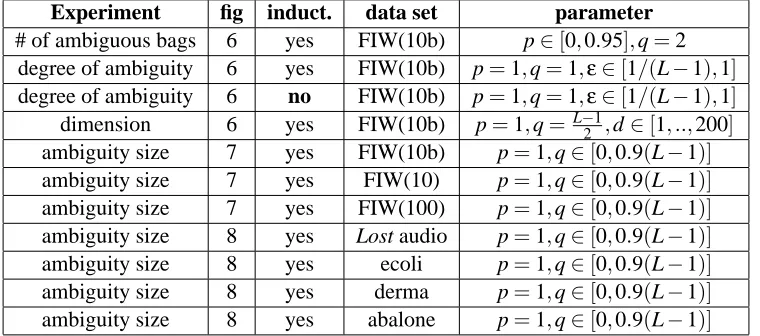
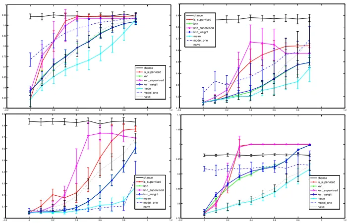
example.3 We also vary the dimensionality by increasing the number of PCA components from 1 to 200, with half of extra labels added uniformly at random. In Figure 7, we vary the ambiguity size q for three different subsets of Faces in the Wild. We report results on additional data sets in Figure 8.

Experiment fig induct. data set parameter # of ambiguous bags 6 yes FIW(10b) p_∈[0,0.95],q=2

degree of ambiguity 6 yes FIW(10b) p=1,q=1,ε_∈[1/(L₋1),1]

degree of ambiguity 6 no FIW(10b) p=1,q=1,ε_∈[1/(L₋1),1]

dimension 6 yes FIW(10b) p=1,q= L−1

2 ,d∈[1, ..,200] ambiguity size 7 yes FIW(10b) p=1,q_∈[0,0.9(L₋1)]

ambiguity size 7 yes FIW(10) p=1,q_∈[0,0.9(L₋1)]

ambiguity size 7 yes FIW(100) p=1,q_∈[0,0.9(L₋1)]

ambiguity size 8 yes Lost audio p=1,q_∈[0,0.9(L₋1)]

ambiguity size 8 yes ecoli p=1,q_∈[0,0.9(L₋1)]

ambiguity size 8 yes derma p=1,q_∈[0,0.9(L₋1)]

ambiguity size 8 yes abalone p=1,q∈[0,0.9(L−1)]

Table 3: Summary of controlled experiments. We experiment with 3 different noise models for ambiguous bags, parametrized by p,q,ε. p represents the proportion of examples that are ambiguously labeled. q represents the number of extra labels for each ambiguous example (generated uniformly without replacement).εrepresents the degree of ambiguity for each ambiguous example (see definition 1). L is the total number of labels. We also study the effects of data set choice, inductive vs transductive learning, and feature dimensionality.

7.3.1 EXPERIMENTS WITH ABOOSTINGVERSION OFCLPL

We also experiment with a boosting version of our CLPL optimization, as presented in Appendix A. Results are shown in Figure 9, comparing our method with kNN and the naive method (also using boosting). Despite the change in learning algorithm and loss function, the trends remain the same.

7.4 Comparative Summary

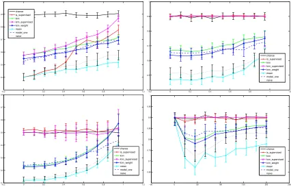
We can draw several conclusions. Our proposed CLPL model uniformly outperformed all base-lines in all but one experiment (UCI dermatology data set), where it ranked second closely behind Model 1. In particular CLPL always uniformly outperformed the naive model. The naive model ranks in second. As expected, increasing ambiguity size monotonically affects error rate. We also see that increasingεsignificantly affects error, even though the ambiguity size is constant, consis-tent with our bounds in Section 3.3. We also note that the supervised models defined in Section 7.1.6 (which ignore the ambiguously labeled examples) consistently perform worse than their coun-terparts adapted for the ambiguous setting. For example, in Figure 6 (Top Left), a model trained with nearly all examples ambiguously labeled (“mean” curve”, p=95%) performs as good as a model which uses 60% of fully labeled examples (“supervised” curve, p=40%). The same holds between the “kNN” curve at p=95% and the “supervised kNN” curve at p=40%.

3. We first choose at random for each label a dominant co-occurring label which is sampled with probabilityε; the rest

−0.2 0 0.2 0.4 0.6 0.8 1 1.2 0.4 0.5 0.6 0.7 0.8 0.9 1 chance is_supervised knn knn_supervised knn_weight mean model_one naive

−0.2 0 0.2 0.4 0.6 0.8 1 1.2

0.4 0.5 0.6 0.7 0.8 0.9 1 chance is_supervised knn knn_supervised knn_weight mean model_one naive

−0.2 0 0.2 0.4 0.6 0.8 1 1.2

0.1 0.2 0.3 0.4 0.5 0.6 0.7 0.8 chance is_supervised knn knn_supervised knn_weight mean model_one naive

−50 0 50 100 150 200 250

0.65 0.7 0.75 0.8 0.85 0.9 0.95 1 chance is_supervised knn knn_supervised knn_weight mean model_one naive

Figure 6: Results on Faces in the Wild in different settings, comparing our proposed CLPL (denoted as mean) to several baselines. In each case, we report the average error rate (y-axis) and standard deviation over 20 trials as in Figure 7. (top left) increasing proportion of am-biguous bags q, inductive setting. (top right) increasing ambiguity degreeε(Equation 1), inductive setting. (bottom left) increasing ambiguity degreeε(Equation 1), transductive setting. (bottom right) increasing dimensionality, inductive setting.

−0.2 0 0.2 0.4 0.6 0.8 1 1.2 0.4 0.5 0.6 0.7 0.8 0.9 1 chance is_supervised knn knn_supervised knn_weight mean model_one naive discriminative_EM

−0.2 0 0.2 0.4 0.6 0.8 1 1.2 0.2 0.3 0.4 0.5 0.6 0.7 0.8 0.9 1 1.1 1.2 chance is_supervised knn knn_supervised knn_weight mean model_one naive

−0.2 0 0.2 0.4 0.6 0.8 1 1.2 0.65 0.7 0.75 0.8 0.85 0.9 0.95 1 chance is_supervised knn knn_supervised knn_weight mean model_one naive

Figure 7: Additional results on Faces in the Wild, obtained by varying the ambiguity size q on the x-axis (inductive case). Left: balanced data set using 50 faces for each of the top 10 labels. Middle: unbalanced data set using all faces for each of the top 10 labels. Right: unbalanced data set using up to 100 faces for each of the top 100 labels.

7.4.1 COMPARISON WITHVARIANTS OFOURAPPROACH

In order to get some intuition on CLPL (Equation 2), which we refer to as the mean model in our experiments, we also compare with the following sum and contrastive alternatives:

L

∑

a∈y

ga(x) !

+

∑

a∈/y

ψ(₋ga(x)), (6)

L

∑

∑

−0.2 0 0.2 0.4 0.6 0.8 1 1.2 0.5 0.55 0.6 0.65 0.7 0.75 0.8 0.85 0.9 0.95 1 chance is_supervised knn knn_supervised knn_weight mean model_one naive

−0.2 0 0.2 0.4 0.6 0.8 1 1.2 0.1 0.2 0.3 0.4 0.5 0.6 0.7 0.8 0.9 1 chance is_supervised knn knn_supervised knn_weight mean model_one naive

−0.20 0 0.2 0.4 0.6 0.8 1 1.2 0.1 0.2 0.3 0.4 0.5 0.6 0.7 0.8 0.9 chance is_supervised knn knn_supervised knn_weight mean model_one naive

−0.2 0 0.2 0.4 0.6 0.8 1 1.2 0.75 0.8 0.85 0.9 0.95 1 1.05 1.1 chance is_supervised knn knn_supervised knn_weight mean model_one naive

Figure 8: Inductive results on different data sets. In each case, we report the average error rate (y-axis) and standard deviation over 20 trials as in Figure 7. Top Left: speaker identification from Lost audio. Top Right: ecoli data set (UCI). Bottom Left: dermatology data set (UCI). Bottom Right: abalone data set (UCI).

Figure 9: Left: We experiment with a boosting version of the ambiguous learning, and compare to a boosting version of the naive baseline (here with ambiguous bags of size 3). We plot accuracy vs number of boosting rounds. The green horizontal line corresponds to the best performance (across k) of the k-NN baseline. Middle: accuracy of k-NN base-line across k. Right: we compare CLPL (labeled mean) with two variants defined in Equation 6,Equation 7, along with the naive model (same setting as Figure 6, Top Left).

Figure 10: Predictions on Lost and C.S.I.. Incorrect examples are: row 1, column 3 (truth: Boone); row 2, column 2 (truth: Jack).

8. Experiments with Partially Labeled Faces in Videos

We now return to our introductory motivating example, naming people in TV shows (Figure 1, right). Our goal is to identify characters given ambiguous labels derived from the screenplay. Our data consists of 100 hours of Lost and C.S.I., from which we extract ambiguously labeled faces to learn models of common characters. We use the same features, learning algorithm and loss function as in Section 7.2.2. We also explore using additional person- and movie-specific constraints to improve performance. Sample results are shown in Figure 10.

8.1 Data Collection

We adopt the following filtering pipeline to extract face tracks, inspired by Everingham et al. (2006): (1) Run the off-the-shelf OpenCV face detector over all frames, searching over rotations and scales. (2) Run face part detectors4over the face candidates. (3) Perform a 2D rigid transform of the parts to a template. (4) Compute the score of a candidate face s(x) as the sum of part detector scores plus rigid fit error, normalizing each to weight them equally, and filtering out faces with low score. (5) Assign faces to tracks by associating face detections within a shot using normalized cross-correlation in RGB space, and using dynamic programming to group them together into tracks. (6) Subsample face tracks to avoid repetitive examples. In the experiments reported here we use the best scoring face in each track, according to s(x).

Concretely, for a particular episode, step (1) finds approximately 100,000 faces, step (4) keeps approximately 10,000 of those, and after subsampling tracks in step (6) we are left with 1000 face examples.

8.2 Ambiguous Label Selection

Screenplays for popular TV series and movies are readily available for free on the web. Given an alignment of the screenplay to frames, we have ambiguous labels for characters in each scene: the set of speakers mentioned at some point in the scene, as shown in Figure 1. Alignment of screenplay to video uses methods presented in Cour et al. (2008) and Everingham et al. (2006), linking closed captions to screenplay.

Lost (#labels, #episodes) (8,16) (16,8)† (16,16) (32,16) Naive 14% 18.6% 16.5% 18.5% ours (CLPL / “mean”) 10% 12.6% 14% 17%

ours+constraints 6% n/a 11% 13%

Table 4: Misclassification rates of different methods on TV show Lost. In comparison, for (16,16) the baseline performances are knn: 30%; Model 1: 44%; chance: 53%. †: This column contains results exactly reproducible from our publicly available reference implementa-tion, which can be found athttp://vision.grasp.upenn.edu/video. For simplicity, this public code does not include a version with extra constraints.

We use the ambiguous sets to select face tracks filtered through our pipeline. We prune scenes which contain characters other than the set we choose to focus on for experiments (top_{8,16,32_} characters), or contain 4 or more characters. This leaves ambiguous bags of size 1, 2 or 3, with an average bag size of 2.13 for Lost, and 2.17 for C.S.I..

8.3 Errors in Ambiguous Label Sets

In the TV episodes we considered, we observed that approximately 1% of ambiguous label sets were wrong, in that they didn’t contain the ground truth label of the face track. This came from several reasons: presence of a non-english speaking character (Jin Kwon in Lost, who speaks Ko-rean) whose dialogue is not transcribed in the closed captions; sudden occurence of an unknown, uncredited character on screen, and finally alignment problems due to large discrepencies between screenplay and closed captions. While this is not a major problem, it becomes so when we con-sider additional cues (mouth motion, gender) that restrict the ambiguous label set. We will see how we tackle this issue with a robust confidence measure for obtaining good precision recall curves in Section 8.5.

8.4 Results with the Basic System

0.52381 0.48039 0.45521 0.45317 0.45098 0.44231 0.35417 0.44231 0.46667 0.49454 0.5641 0.43939 0.46032 0.45455 0.35714 0.38889 0.91667 0.94118 0.8625 0.84298 1 0.88462 0.8125 0.94872 1 0.90164 0.96154 0.72727 0.33333 0.81818 0.28571 0 Jack John Charlie Kate James Boone Hurley Sayid Michael Claire Sun Walt Liam Shannon Jin Ethan

Figure 11: Left: Label distribution of top 16 characters in Lost (using the standard matlab color map). Element Di j represents the proportion of times class i was seen with class j in

the ambiguous bags, and D1=1. Right: Confusion matrix of predictions from Section 8.4. Element Ai j represents the proportion of times class i was classified as class j, and

A1=1. Class priors for the most frequent, the median frequency, and the least frequent characters in Lost are Jack Shephard, 14%; Hugo Reyes, 6%; Liam Pace 1%.

Quantitative results are shown in Table 4. We measure error according to average 0-1 loss with respect to hand-labeled groundtruth labeled in 8 entire episodes of Lost. Our model outperforms all the baselines, and we will further improve results. We now compare several methods to obtain the best possible precision at a given recall, and propose a confidence measure to this end.

8.5 Improved Confidence Measure for Precision-recall Evaluation

We obtain a precision-recall curve using a refusal to predict scheme, as used by Everingham et al. (2006): we report the precision p for the r most confident predictions, varying r_∈[0,1]. We com-pare several confidence measures based on the classifier scores g(x)and propose a novel one that significantly improves precision-recall, see Figure 12 for results.

1. the max and ratio confidence measures (as used in Everingham et al., 2006) are defined as:

Cmax(g(x)) =max

a ga(x),

Cratio(g(x)) =max

a

exp(ga(x))

∑bexp(gb(x))

.

2. the relative score can be defined as the difference between the best and second best scores over all classifiers(ga)a∈{1..L}(where a∗=arg maxa∈{1..L}ga(x)):

Crel(g(x)) =ga∗(x)− max

a∈{1..L}−{a∗_}ga(x).

3. we can define the relative-constrained score as an adaptation to the ambiguous setting; we only consider votes among ambiguous labels y (where a∗=arg max_a∈yga(x)):

Crel,y(g(x)) =ga∗(x)− max

0 0.2 0.4 0.6 0.8 1 0

0.05 0.1 0.15 0.2 0.25 0.3 0.35

max ratio relative relative constrain hybrid

Figure 12: Improved hybrid confidence measure for precision-recall evaluation. x axis: recall; y axis: naming error rate for CLPL on 16 episodes of Lost (top 16 characters). max confidence score performs rather poorly as it ignores other labels. relative improves the high precision/low recall region by considering the margin instead. The relative-constrain improves the high-recall/low-precision region by only voting among the am-biguous bags, but it suffers in high-precision/low recall region because some amam-biguous bags may be erroneous. Our hybrid confidence score gets the best of both worlds.

There are some problems with all of those choices, especially in the case where we have some errors in ambiguous label set (a_∈/Y for the true label a). This can occur for example if we restrict them with some heuristics to prune down the amount of ambiguity, such as the ones we consider in Section 8.6 (mouth motion cue, gender, etc). At low recall, we want maximum precision, therefore we cannot trust too much the heuristic used in relative-constrained confidence. At high recall, the errors in the classifier dominate the errors in ambiguous labels, and relative-constrained confidence gives better precision because of the restriction. We introduce a hybrid confidence measure that performs well for all recall levels r, interpolating between the two confidence measures:

ha_r(x) =

(

ga(x) if a∈y,

(1₋r)ga(x) +r minbgb(x) else.

Cr(g(x)) =Crel(hr(x)).

By design, in the limit r_→0, Cr(g(x))≈Crel(g(x)). In the limit r→1, har(x)is small for a∈/y and

so Cr(g(x))≈Crel,y(g(x)).

8.6 Additional Cues

8.6.1 MOUTHMOTION

We use a similar approach to Everingham et al. (2006) to detect mouth motion during dialog and adapt it to our ambiguous label setting.5 For a face track x with ambiguous label set y and a tem-porally overlapping utterance from a speaker a_{∈ {}1..L_}(after aligning screenplay and closed cap-tions), we restrict y as follows:

y :=

  

 

{a_} if mouth motion,

y if refuse to predict or y=_{a_}, y_{− {}a_} if absence of mouth motion.

8.6.2 GENDERCONSTRAINTS

We introduce a gender classifier to constrain the ambiguous labels based on predicted gender. The gender classifier is trained on a data set of registered male and female faces, by boosting a set of decision stumps computed on Haar wavelets. We use the average score over a face track output by the gender classifier. We assume known the gender of names mentioned in the screenplay (using automatically extracted cast list from IMDB). We use gender by filtering out the labels that do not match by gender the predicted gender of a face track, if the confidence exceeds a threshold (one for females and one for males are set on a validation data to achieve 90% precision for each direction of the gender prediction). Thus, we modify ambiguous label set y as:

y :=

  

 

y if gender uncertain, y_{− {}a : a is male_} if gender predicts female,

y− {a : a is female} if gender predicts male.

8.6.3 GROUPINGCONSTRAINTS

We propose a very simple must-not-link constraint, which states yi6=yj if face tracks xi,xj are in

two consecutive shots (modeling alternation of shots, common in dialogs). This constraint is active only when a scene has 2 characters. Unlike the previous constraints, this constraint is incorporated as additional terms in our loss function, as in Yan. et al. (2006). We also propose groundtruth grouping constraints for comparison: yi=yjfor each pair of face tracks xi,xjof the same label, and

that are separated by at most one shot.

8.7 Ablative Analysis

Figure 13 is an ablative analysis, showing error rate vs recall curves for different sets of cues. We see that the constraints provided by mouth motion help most, followed by gender and link constraints. The best setting (without using groundtruth) combines the former two cues. Also, we notice, once again, a significant performance improvement of our method over the naive method.

8.8 Qualitative Results and Video Demonstration

We show examples with predicted labels and corresponding accuracy, for various characters in C.S.I., see Figure 14. Those results were obtained with the basic system of Section 8.4. Full-frame