R E S E A R C H
Open Access
A robust information source estimator with
sparse observations
Kai Zhu
*and Lei Ying
*Correspondence: [email protected] School of Electrical, Computer and Energy Engineering, Arizona State University, Tempe, AZ 85287, USA
Abstract
Purpose/Background: In this paper, we consider the problem of locating the information source with sparse observations. We assume that a piece of information spreads in a network following a heterogeneous susceptible-infected-recovered (SIR) model, where a node is said to beinfectedwhen it receives the information and recoveredwhen it removes or hides the information. We further assume that a small subset of infected nodes are reported, from which we need to find the source of the information.
Methods: We adopt the sample path-based estimator developed in the work of Zhu and Ying (arXiv:1206.5421, 2012) and prove that on infinite trees, the sample
path-based estimator is a Jordan infection center with respect to the set of observed infected nodes. In other words, the sample path-based estimator minimizes the maximum distance to observed infected nodes. We further prove that the distance between the estimator and the actual source is upper bounded by a constant independent of the number of infected nodes with a high probability on infinite trees. Results: Our simulations on tree networks and real-world networks show that the sample path-based estimator is closer to the actual source than several other algorithms.
Conclusions: In this paper, we proposed the sample path-based estimator for information source localization. Both theoretic analysis and numerical evaluations showed that the sample path-based estimator is robust and close to the real source.
Keywords: Information source detection; Heterogeneous SIR model; Sparse observation
Background
In this paper, we are interested in locating the source of information that spreads in a network by using sparse observations. The solution to this problem has important appli-cations such as locating the sources of epidemics, the sources of news/rumors in social networks, or the sources of online computer virus. The problem has been studied in [1-5] under a homogeneous susceptible-infected (SI) model for information diffusion and in [6] under a homogeneous susceptible-infected-recovered (SIR) model for information diffusion, assuming that a complete snapshot of the network is given.
While [1-6] answered some basic questions about information source detection in large-scale networks, a complete snapshot of a real-world network, which may have
hundreds of millions of nodes, is expensive to obtain. Furthermore, these works assume homogeneous infection across links and homogeneous recovery across nodes, but in reality, most networks are heterogeneous. For example, people close to each other are more likely to share rumors, and epidemics are more infectious in the regions with poor medical care systems. Therefore, it is important to take sparse observations and network heterogeneity into account when locating information sources. In this paper, we assume that the information spreads in the network following a heterogeneous SIR model and assume that only a small subset of infected nodes are reported to us. The goal is to identify the information source in a heterogeneous network by using sparse observations.
We use the sample path-based approach developed in [6] for locating the information source with sparse observations. Surprisingly, we find that the sample path-based esti-mator is robust to network heterogeneity and the number of observed infected nodes. In particular, our results show that even under a heterogeneous SIR model and with sparse observations, the sample path-based estimator remains to be a Jordan infection center in infinite trees, where the Jordan infection centers with a partial observation are the nodes that minimize the maximum distance to observed infected nodes. We further show that in an infinite tree, the distance between a Jordan infection center and the actual source can be bounded by a value independent of the size of an infected subnetwork with a high probability, where the infected subnetwork is the subnetwork consisting of nodes which are either infected or recovered, and is a connected component. Assume that the size of the infected subnetwork isn, and the result says that a Jordan infection center is a distance ofO(1)from the actual source.
We remark that the locations of the Jordan centers only depend on the network topology and are independent of the infection and recovery probabilities, so the sample path-based estimators (or the Jordan infection centers) are also robust to the information diffusion model, which makes it very appealing in practice since the accurate knowledge of the SIR parameters can be difficult to measure in reality.
Related works
Methods
A heterogeneous SIR model
In this section, we introduce the heterogeneous SIR model for information propagation. Different from the homogeneous SIR model in which infection and recovery probabilities are both homogeneous [6], the heterogeneous SIR model we consider allows different infection probabilities at different links and different recovery probabilities at different nodes.
Consider an undirected graphG= {V,E}, whereVis the set of nodes andE is the set of edges. Denote by(u,v)∈Ethe edge between nodeuand nodev. Each nodev∈Vhas three states: susceptible (S), infected (I), and recovered (R). A node is said to be suscep-tible if it has not received the information, infected after it receives the information, and recovered if the node removes or hides the information. Time is slotted. At the beginning of each time slot, each infected node attempts to contact all its susceptible neighbors. A contact from nodeuto nodev succeedswith probabilityquv. A susceptible node becomes infected after beingsuccessfullycontacted by one of its infected neighbors. At the middle of each time slot, an infected node,if it is infected before the current time slot,recovers with probabilitypv. A recovered node cannot be infected again. We assume that contacts succeed independently across links and time slots and that nodes recover independently across nodes and time slots.
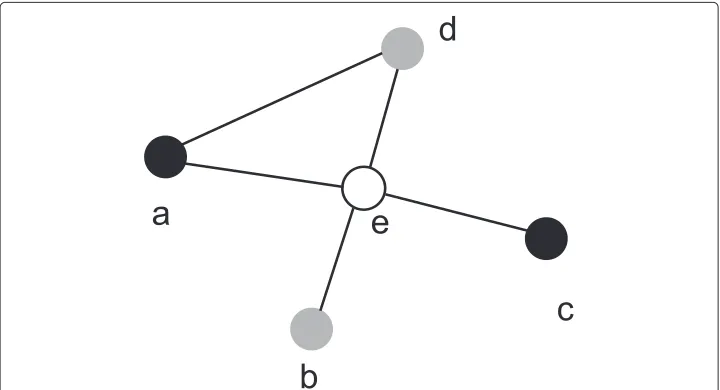
Consider a network shown in Figure 1, where nodeeis in the susceptible state, nodesa
andcare in the infected state, and nodesbanddare in the recovered state. Then, at the next time slot, nodeebecomes infected with probability
1−(1−qae)(1−qce),
and nodesaandcrecover with probabilitypaandpc, respectively.
Problem formulation
In this section, we formally define the problem of information source detection. Table 1 summarizes the notations used in the paper. Adopting the notation in [6], we defineXv(t)
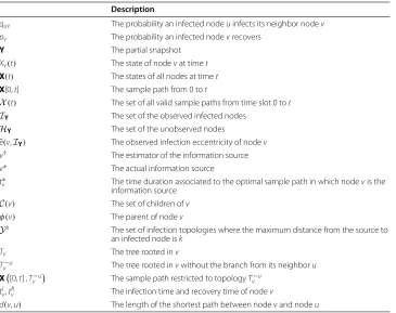
Table 1 Notation table
Description
quv The probability an infected nodeuinfects its neighbor nodev
pv The probability an infected nodevrecovers
Y The partial snapshot
Xv(t) The state of nodevat timet
X(t) The states of all nodes at timet
X[0,t] The sample path from 0 tot
X(t) The set of all valid sample paths from time slot 0 tot
IY The set of the observed infected nodes
HY The set of the unobserved nodes
˜
e(v,IY) The observed infection eccentricity of nodev
v† The estimator of the information source
v∗ The actual information source
t∗v The time duration associated to the optimal sample path in which nodevis the information source
C(v) The set of children ofv
φ(v) The parent of nodev
Yk The set of infection topologies where the maximum distance from the source to
an infected node isk
Tv The tree rooted inv
T−u
v The tree rooted invwithout the branch from its neighboru
X[0,t] ,T−u v
The sample path restricted to topologyT−u v
tIv,tRv The infection time and recovery time of nodev
d(v,u) The length of the shortest path between nodevand nodeu
to be the states of nodevat the end of time slottsuch that
Xv(t)=
⎧ ⎪ ⎨ ⎪ ⎩
S, ifvis in state S at timet; I, ifvis in state I at timet; R, ifvis in state R at timet.
LetX(t)= {Xv(t):∀v∈V}denote the states of all nodes at time instantt.
In this paper, we assume that we only haveone partial snapshotof the network, which is
a subset of the infected nodes.This observation can be sparse, and details will be given in the next section. We assume that the states of other nodes are unknown. We letYvdenote the state of nodevin the snapshot such that
Yv=
1, if nodevis observed to be infected; 0, otherwise.
LetY = {Yv : ∀v ∈ V}. We denote byv∗ the information source. The problem of information source detection is to locatev∗based on the partial observationYand the network topologyG.
Due to recovery and partial observations, all nodes in the network are potential can-didates of the information source. The maximum likelihood estimator of the problem is therefore computationally expensive to find as pointed out in [6]. In this paper, we follow the sample path-based approach proposed in [6] to find an estimator ofv∗.
which is the states of all nodes from time 0 to timet. We further define a functionF(·)
such that
F(Xv(t))=
1, ifXv(t)=Iandvis observed; 0, otherwise.
This function maps the actual state of a node to the observed state of the node. F(X(t)) = Yif and only ifF(Xv(t)) = Yv,∀v ∈ V. The optimal sample pathX∗[0,t∗] is defined to be the most likely sample path that results in the observed snapshot, i.e., it solves the following optimization problem:
X∗[0,t∗]=arg maxt,X[0,t]∈X(t)Pr(X[0,t]), (1)
whereX(t)= {X[0,t]|F(X(t))=Y}and Pr(X[0,t])is the probability that the sample path X[0,t] occurs. The source that associates withX∗[0,t∗] is calledthe sample path-based estimator. It is proved in [6] that the sample path-based estimator on an infinite tree is a Jordan infection center under the homogeneous SIR model with a complete snapshot. The focus of this paper is to identify the sample path-based estimator under the heterogeneous SIR model with sparse observations.
Main results
In this section, we summarize the main results of this paper.
Main result 1: the Jordan infection centers as the sample path-based estimators
In our theoretical analysis, we consider tree networks with infinitely many levels (or called infinite trees) to derive the sample path-based estimator under the heterogeneous SIR model with a partial snapshot. LetIY denote the set of observed infected nodes. We
define the observed infection eccentricity˜e(v,IY)of nodevto be the maximum distance
betweenvand any observed infected node where the distance is defined to be the short-est distance between two nodes. The Jordan infection centers of the partial snapshot are then defined to be the nodes with the minimum observed infection eccentricity. The fol-lowing theorem states that on an infinite tree, the sample path-based estimator is a Jordan infection center of the partial snapshot.
Theorem 1.Consider an infinite tree and assume that the partial snapshotYcontains at least one infected node. The sample path-based estimator, denoted by v†,is a Jordan infection center, i.e.,
v†∈arg min
v∈Ve˜(v,IY). (2)
The proof of this theorem consists of the following key steps.
t≥ ˜e(v,IY),the sample path with the highest probability inXv(t)occurs more likely than the one inXv(t+1).In other words,
max
X[0,t]∈Xv(t)Pr(X[ 0,t]) >X[0,t+max1]∈Xv(t+1)Pr(X[0,t+1]).
As a consequence of this result, we conclude thatthe sample path that has the highest probability among those originated from nodevhas a duration of˜e(v,IY) (the observed infection eccentricity of nodev). This result will be proved in Lemma 1 in the ‘Proofs’ section.
2. In the second step, we consider two neighboring nodes, say nodesuandv, and assume nodevhas a smaller observed infection eccentricity than nodeu.Based on Lemma 1, we will prove that the optimal sample path associated with nodev occurs with a higher probability than that of nodeu.The key idea is to construct a sample path originated from nodevbased on the optimal sample path originated from nodeuand show that it occurs with a higher probability. This result will be proved in Lemma 2 in the ‘Proofs’ section.
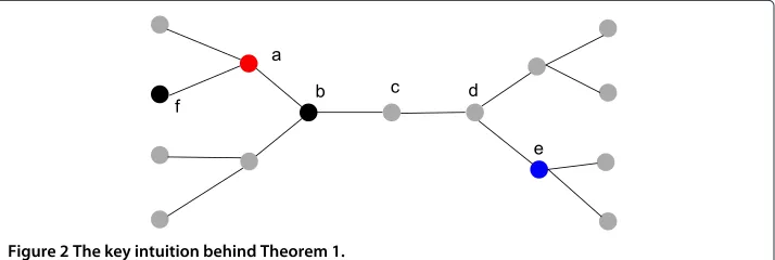
3. We will finally prove that starting from any node, there exists a path from the node to a Jordan infection center such that the observed infection eccentricity strictly decreases along the path. Consider an example in Figure 2. Nodesbandf are two observed infected nodes. So nodeais a Jordan infection center with observed infection eccentricity 1. The path from nodeeto nodeais
e→d→c→b→a,
along which the observed infection eccentricity decreases as
5→4→3→2→1.
By repeatedly using Lemma 2, it can be shown that the optimal sample path originated from a Jordan infection center occurs with a higher probability than the optimal sample path originated from a node which is not a Jordan infection center, which implies that the sample path-based estimator must be a Jordan infection center.
Main result 2: anO(1)bound on the distance between a Jordan infection center and the actual information source
Unlike the maximum likelihood estimator, the sample path estimator does not guarantee that the estimator is the node that most likely leads to the observation. It has been shown in [6] that on tree networks and under the homogeneous SIR model, the distance between
the estimator and the actual source is a constant with a high probability. It is easy to see that with a partial observation, the distance between the estimator and the actual source cannot be bounded if the observed infection nodes are arbitrarily chosen. In this paper, we consider a class of fairly general sampling algorithms that generate the partial observation (and maybe sparse). The sampling algorithms have the following property:for any set of M infected nodes, the probability that at least one node in the set is reported approaches to 1 as M goes to infinity.We call such a sampling algorithmunbiased; in other words, any subset of infected nodes is likely to contain an observed infected node when the size of the subset is large enough. Note that if an infected node is reported with probability at leastδfor someδ >0, independent of other nodes, then it satisfies the property above. Our second main result is that the sample path estimator is within a constant distance from the actual source independent of the size of the infected subnetwork if the sampling algorithm is unbiased.We also emphasize that the observation generated by an unbiased sampling algorithm can be very sparse since we only require that one observed infected node is reported with a high probability among M nodes when M is sufficiently large.
Theorem 2.Consider an infinite tree. Let gminbe the lower bound on the number of
children and qmin > 0be the lower bound on q.Assume gmin > 1,gminqmin > 1,and
the observed infection topologyYcontains at least one infected node and is generated by an unbiased sampling algorithm. Then given > 0, the distance between the sample path estimator and the actual source is d with probability1−,where d is indepen-dent of the size of the infected subnetwork. In other words, the distance is O(1)with a high probability.
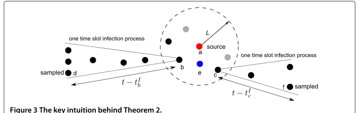
The idea of the proof is illustrated using Figure 3, which consists of the following key steps:
1. We first define a one-time-slot infection subtree to be a subtree of the infected subnetwork such that each node on the subtree is infected in the next time slot after the parent is infected, except the source node. Note that the depth of a one-time-slot infection subtree grows by 1 deterministically until it terminates. We further say a node survives at timetif it is the root of a one-time-slot infection subtree which has not terminated by timet.
2. In the first step, we will prove that there exist at least two survived nodes within a distanceLfrom the information source. In Figure 3, nodeais the information source, and nodesbandcare two survived nodes.
3. In the second step, we will show that with a high probability, at least one infected node at the bottom of a one-time-slot infection subtree, which has not terminated, is observed under an unbiased sampling algorithm. In Figure 3, nodesdandf are two sampled nodes corresponding to the two one-time-slot infection subtrees starting from nodesbandc,respectively.
4. Since a one-time-slot infection subtree grows by 1 deterministically at each time slot, the depth of a one-time-slot infection subtree ist−tkI,wherekis the root node of the one-time-slot infection subtree. Recall that the Jordan infection centers minimize the maximum distance to observed infected nodes, so a Jordan infection center must be within aO(1)distance from the two survived nodes (nodesbandc). Considering Figure 3, we know that the actual source (nodea) has an infection eccentricity≤tsince the information can propagate at mostthops at timet.So the infection eccentricity of the Jordan infection centers is no more thant
according to the definition. Assume nodeein Figure 3 is a Jordan infection center, then it is within a distance ofO(t)from nodesdandf,and so is within a distance ofO(1)from nodesbandc.Since nodesbandcare no more thanLhops from the actual sourcea,we can conclude that the distance between the actual sourceaand the estimatoreisO(1).
Reverse infection algorithm
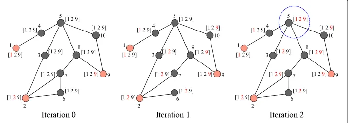
The Jordan infection centers for general graphs can be identified by the reverse infec-tion algorithm proposed in [6]. In the algorithm, each observed infected node broadcasts its identity (ID) to its neighbors. All nodes in the network record the distinct IDs they received. When a node receives a new distinct ID, it records it and then broadcasts it to its neighbors. This process stops when there is a node which receives the IDs from all observed infected nodes. It is easy to verify that the set of nodes which first receive all infected IDs is the set of Jordan infection centers. When there are multiple Jordan infection centers in the graph, we select the one with the maximum infection close-ness centrality as the information center. The infection closeclose-ness centrality is defined as the inverse of the sum of the distances from one node to all observed infected nodes.
We explain the reverse infection algorithm using an example in Figure 4. The red nodes are the observed infected nodes, and the black nodes are the unobserved nodes. The array next to each node records the IDs that the node has received. When an ID is received, it
is colored in red. For example, node 7 in iteration 1 has received the ID of node 2 which is colored in red and has not received the ID of nodes 1 and 9 which are in black. At each iteration, each node broadcasts its newly received IDs to its neighbors. For exam-ple, node 4 just received the ID of node 1 in iteration 1 so it will broadcast node 1’s ID to its neighbors in iteration 2. The algorithm terminates when some nodes receive the IDs of all observed infected nodes, and this node is the Jordan infection center. In iteration 3, node 5 received all IDs and so node 5 is the Jordan infection center in the example.
Discussion: robustness
According to the two main results above, we know that the sample path-based esti-mator remains to be a Jordan infection center. This is a somewhat surprising result since the locations of the Jordan infection centers are determined by the topology of
the network and are independent of the parameters of the heterogeneous SIR model.
In other words, the locations of the Jordan infection centers remain the same for different SIR processes as long as the set of observed infected nodes is the same. This property suggests that the sample path-based estimator is a robust estimator and can be used in the case when the parameters of the SIR model are unknown, which is a very desirable property since knowing these parameters can be difficult in practice.
In the simulations, we also consider a weighted graph with the link weights chosen proportionally according to the SIR parameters and use the weighted Jordan infection centers as the estimator. Interestingly, we will see that the performance is worse than the unweighted Jordan infection centers, which again demonstrates the robustness of the sample path-based estimator.
Furthermore, the main results hold as long as the sampling algorithm is unbiased and are independent of the number of samples. So the results are valid for sparse observations and are robust to the number of observations.
Results and discussion Simulations
In this section, we evaluate the performance of the reverse infection algorithm for the heterogeneous SIR model on different networks including tree networks and real-world networks.
We first describe the heterogeneous SIR model we used in the simulation. Each edge
e ∈ Eis assigned with a weightqewhich is uniformly distributed over(0, 1). The infec-tion time over each edgee ∈ E is geometrically distributed with mean 1/qe. Similarly, each nodev ∈ V is assigned with a weightpvgenerated by a uniform distribution over (0, 1), and the recovery time is geometrically distributed with mean 1/pv. The informa-tion source is randomly selected. The total number of infected and recovered nodes in each infection graph is within the range of [100, 300]. Each infected nodevin the infection graph reports with probabilityσ, independently. The snapshots used in the simulations have at least one infected node. We changedσand evaluated the performance on different networks.
1. Closeness centrality algorithm (CC) : The closeness centrality algorithm selects the node with the maximum infection closeness as the information source.
2. Weighted reverse infection algorithm (wRI) : The weighted reverse infection algorithm selects the node with the minimum weighted infection eccentricity as the information source where the weighted infection eccentricity is similar to the infection eccentricity except that the length of a path is defined to be the sum of the link weights instead of the number of hops, and the link weight is the average time it takes to spread the information over the link, i.e., 1/qe
on edgee. 3. Weighted closeness centrality algorithm (wCC) : The weighted closeness centrality
algorithm selects the node with the maximum weighted infection closeness as the information source.
Tree networks
We first evaluated the performance of the RI algorithm on tree networks.
Regular trees A g-regular tree is a tree where each node hasg neighbors. We set the degreeg=5 in our simulations.
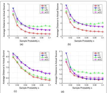
We varied the sample probabilityσ from 0.01 to 0.1. The simulation results are sum-marized in Figure 5a, which shows the average distance between the estimator and the actual information source versus the sampling probability. When the sample probability increases, the performance of all algorithms improves. When the sample probability is
larger than 6%, the average distance becomes stable which means that a small number of infected nodes is enough to obtain a good estimator. We also notice that the average dis-tance of RI is smaller than all other algorithms and is less than one hop whenσ ≥0.04. wRI has a similar performance with RI when the sample probability is small (=0.01) but becomes much worse when the sample probability increases.
Binomial trees We further evaluated the performance of RI and other algorithms on binomial treesT(ξ,β)where the number of children of each node follows a binomial distribution such thatξ is the number of trials andβ is the success probability of each trial. In the simulations, we selectedξ =10 andβ = 0.4. Again, we variedσ from 0.01 to 0.1. The results are shown in Figure 5b. Similar to the regular trees, the performance of RI dominates CC, wRI, and wCC, and the difference in terms of the average number of hops is approximately 1 whenσ ≥0.03.
Real-world networks
In this section, we conducted experiments on two real-world networks: the Internet autonomous systems (IAS) network which is available at http://snap.stanford.edu/data/ index.html and the power grid (PG) network which is available at http://www-personal. umich.edu/~mejn/netdata/.
The power grid network The power grid network has 4,941 nodes and 6,594 edges. On average, each node has 1.33 edges. So the power grid network is a sparse network. The simulation results are shown in Figure 5c. In the power grid network, we can see that RI and wRI have similar performance, and both outperform CC and wCC by at least one hop
whenσ≥0.04.
The internet autonomous systems network The Internet autonomous systems net-work is the data collected on 31 March 2001. There are 10,670 nodes and 22,002 edges in the network. The simulation results are shown in Figure 5d. wRI and wCC always per-form worse than RI. Although RI and CC have similar perper-formance when the sample probability is large, RI outperforms CC whenσ ≤0.03.
RI versus DMP
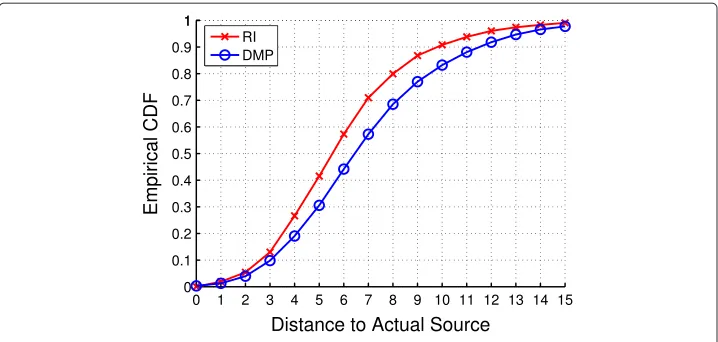
We finally compared the performance of RI and DMP. We conducted the simulation on the power grid network and fixed the sample probability to be 10%. Under this setting, the complexity of DMP is very high since the DMP computation needs to be repeated for every node in the network. Since nodes far away from the observed infected nodes are not likely to be the information source, we ran DMP over a small subset of nodes close to the Jordan infection centers (roughly 10%) to reduce the complexity of the algorithm.
We tested the speed of RI and DMP on a machine with 1.8 GB memory, 4 cores 2.4 GHz Intel i5 CPU and Ubuntu 12.10. The algorithms are implemented in Python 2.7. On average, it took RI 0.57 s to locate the estimator for one snapshot and took DMP 229.12 s. So RI is much faster than DMP.
Figure 6 The CDF of RI and DMP on the power grid network.
source compared to 57% under DMP. Therefore, RI outperforms DMP in terms of both speed and accuracy. We remark that we did not compare the performance of RI and DMP on the IAS network because the complexity of running DMP on a large-sized network like the IAS network is prohibitively high.
Proofs
In this section, we present the proofs of the main results.
Proof of Theorem 1
Denote byIY = {v|Yv=1}the set of observed infected nodes andHY= {v|Yv =0}the set of unobserved nodes. Given a nodev, define the optimal timetv∗to be
t∗v argt max
t,X[0,t]∈X(t)Pr(X[ 0,t]|vis information source),
i.e., it is the duration of the optimal sample path with nodevas the information source.
Lemma 1(Time Inequality).Consider an infinite tree rooted at vr.Assume that vris
the information source and the observed snapshotYcontains at least one infected node. If
˜
e(vr,IY)≤t1<t2, the following inequality holds:
max X[0,t1]∈ ˜X(t1)
Pr(X[0,t1]) > max
X[0,t2]∈ ˜X(t2)
Pr(X[0,t2]),
whereX˜(t)= {X[ 0,t]|Y=F(X(t))}.In addition,
t∗vr = ˜e(vr,IY)=max u∈IY
d(vr,u),
i.e., t∗vris equal to the observed infection eccentricity of vrwith respect toIY.
Proof. We adopt the notations defined in [6], which are listed below:
• Ykis the set of infection topologies where the maximum distance fromv rto an infected node isk. All possible infection topologies are then partitioned into countable subsets{Yk}.
• Tvis the tree rooted inv.
• Tv−uis the tree rooted invwithout the branch from its neighboru. • X([0,t] ,T−u
v )is the sample path restricted to topologyTv−u. • tI
v,tRv are the infection time and recovery time of nodev.
Considering the case where the time difference of two sample paths is 1, we will show that
max
X[0,t]∈ ˜X(t)
Pr(X[0,t]) > max
X[0,t+1]∈ ˜X(t+1)
Pr(X[0,t+1]).
Next, we use induction overYk.
Step 1 k=0 vr is the only observed infected node in this case. Given a sample path X[0,t+1]∈ ˜X(t+1), the probability of the sample path can be written as
Pr(X[0,t+1])=Pr(X[0,t])Pr(X(t+1)|X[0,t]).
Sincevr is the only observed infected node and all other nodes’ states are unknown, we assignX[0,t]∈ ˜X(t)to be same as the firstttime slots inX[0,t+1] , i.e.,X[0,t]=X[0,t] . Hence, we obtain that
PrX[0,t]=Pr(X[0,t]) >Pr(X[0,t+1]).
Therefore, the casek=0 is proved.
Step 2Assume the inequality holds fork ≤nand considerk = n+1, i.e.,Y∈Yn+1. Clearly,t≥ n+1 ≥1 for eachX[0,t]. Furthermore, the set of subtreesT = {T−vr
u |u ∈ C(vr)}are divided into two subsets:
Th= {T−vr
u |u∈C(vr),Tu−vr ∩IY= ∅}
and
Ti=T\Th.
GiventRvr, the infection processes on the subtrees are mutually independent.
We construct X[0,t] which occurs more likely than X∗[0,t + 1] according to the following steps, whereX∗[0,t+1]=arg maxX[0,t+1]∈ ˜X(t+1)Pr(X[0,t+1]).
Part 1Ti. For a subtree inTithe proof follows Step 2.b and Step 2.c of Lemma 1 in [6]. The intuition is as follows: Consider a subtree and a sample path on it with durationt+1. Ifuis not infected at the first time slot, we can construct a sample path with durationt
by moving the events one time slot earlier. The new sample path (with durationt) has a higher probability to occur than the original one. Ifuis infected in the first time slot, we can invoke the induction assumption to the subtree rooted atu, which belongs toYn.
Part 2 vr. In this part, we have the freedom to assign the unobserved node as infected or healthy. In part 1, the infection time of each rootuin subtreesTi ofX[0,t] is either the same as or one time slot earlier than its infection time inX∗[0,t+1]. Therefore, if
tRvr ≤t, the recovery time of the sourcevrinX[0,t] can be assigned the same as that in X∗[0,t+1].
IftRvr >t+1,vrremains infected in the sample pathX∗[ 0,t+1]. We assign the source to be in stateIinX[ 0,t].
As a summary, according to the assignment above, the states of the sourcevrinX[0,t] are the same as those of the firstttime slots inX∗[0,t+1].
Part 3Th. Based on the conclusion of part 2, the subtrees belonging toThinX[0,t] mimic the behaviors of the firstttime slots inX∗[0,t+1].
SinceX∗[0,t+1] has one extra time slot during which some extra events occur,X[0,t] occurs with a higher probability on the subtrees inTh.
According to the discussion above, we conclude that time inequality holds fork=n+1 and hence for anykaccording to the principle of induction. Therefore, the lemma holds.
Lemma 2(Adjacent nodes inequality).Consider an infinite tree with partial obser-vationYwhich contains at least one infected node. For u,v ∈ V such that(u,v) ∈ E, if t∗u>tv∗
Pr(X∗u[0,t∗u]) <Pr(X∗v[0,t∗v]),
whereX∗u[0,tu∗]is the optimal sample path associated with root u.
Proof. The proof of the lemma follows the proof of Lemma 2 in [6]. The key idea is to construct a sample path rooted atv, which has a higher probability than the optimal sample path rooted at u. It is not hard to see that tu∗ = t∗v +1 based on the defini-tion of the infecdefini-tion eccentricity. The graph is partidefini-tioned intoTv−u andTu−v which are mutually independent after the infection ofvandu. With this observation, we construct
˜
Xv[0,tv∗] which infectsuat the first time slot.Xv˜ [0,tv∗] ,T−u v
then mimics the behavior of Xu∗[0,t∗u] ,Tv−u, andXv˜ [0,t∗v−1] ,Tu−vhas a higher probability thanX∗u[0,tu∗] ,Tu−v
based on Lemma 1.
The adjacent nodes inequality results in partial orders in the tree and makes it pos-sible to compare the likelihood of optimal sample paths associated with adjacent nodes without knowing the actual probability of the optimal sample path. Following the proof of Theorem 4 in [6], it can be shown that in tree networks, from any node, there exists a path from the node to a Jordan infection center such that the observed infection eccen-tricity strictly decreases along the path. By repeatedly using Lemma 2, we can then prove that the source of the optimal sample path must be a Jordan infection center.
Proof of Theorem 2
In this subsection, we present the proof that shows that the sample path estimator is within a constant distance from the actual source independent of the size of the infected subnetwork. Given a tree rooted inv∗where the information starts fromv∗following the general SIR model, we define the following three branching processes:
1. Zl(Tv∗)denotes the set of nodes which are in infected or recovered states at levell on treeTv∗.LetZl(Tv∗)denote the cardinality ofZl(Tv∗).Note that
Z0(Tv∗)= {v∗}.We call this process theoriginal infection process.
were infected. This process adds a deadlineτon infection. If a node is not infected withinτ time slots after its parent is infected, it is not included in this branching process. This process is calledτ-deadline infection process. From the definition, if u,v∈Zlτ(Tv∗),then
|tIu−tIv| ≤l(τ−1).
Forτ =1,we callZl1(Tv∗)theone-time-slot infection process. The extinction probability of a branching process is the probability that there is no offspring at a certain level of the branching process, i.e.,Z1l(Tv∗)=0for somel.Denote byρv
the extinction probability ofZl1
Tv−φ(v)
.
3. We define thebinomial branching process as a branching process whose offspring distribution follows binomial distributionB(g,ϕ)wheregis the number of trials andϕis the success probability. Denote byρthe extinction probability of the binomial branching process.
The following notations will be used in later analysis:
• v†denotes the optimal sample path estimator.
• gminis the lower bound on the number of children, i.e.,
min
v |C(v)| ≥gmin,∀v∈V.
• qminis the lower bound on the infection probability, i.e.,
qmin=min
e qe,∀e∈E. • στ
v is the probability that a nodevinfects at least one of its children withinτ time slot aftervis infected.
Givenn0>0 andτ >0, definel†=minlwhereZlτ(Tv∗) >n0, i.e.,l†is the first level
where theτ-deadline infection process has more thann0offsprings.
Givenτand levelL≥2, we consider the following two events:
Event 1:ZL(Tv∗)=0.
Event 2:l† ≤ Land at least two one-time-slot infection processes starting from level
l†survive, i.e.,∃u,v∈ Zlτ†(Tv∗)such that∀l,Zl1
Tu−φ(u)
=0 andZl1Tv−φ(v)
=0. In addition, at least one infected node at the bottom of each survived one-time-slot infection process is observed.
For event 1, no node at levelLgets infected and the infection process terminates at level
L−1. So the infection eccentricity ofv∗is at mostL−1, and the minimum infection eccentricity of the network is at mostL−1. Therefore, the distance betweenv∗andv†is no more than 2(L−1).
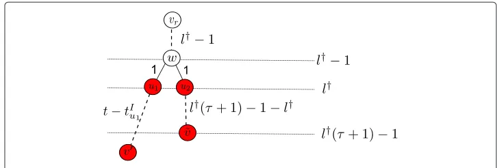
Considering event 2, we assume that the information propagates forttime slots. The deadline property of theτ-deadline infection process indicatestIu1 ≤ τl†andtIu2 ≤ τl†. Given a nodev˜at level(τ+1)l†−1 wherev˜∈T−φ(u2)
u2 and a nodev∈T
−φ(u1)
u1 which is
an observed infected node at the bottom of the infection tree, from Figure 7, we obtain
dv˜,v=t−tIu1+τl†+1≥t+1.
Note that∀u∈I,
Figure 7 A pictorial description of the distance relations in Theorem 2.
Sincel†≤L, any node at or below levelL(τ+1)−1 has an infection eccentricity larger than that ofv∗. Hence,v†cannot be at or below levelL(τ+1)−1. Therefore,
d
v†,v∗
< (τ +1)L−1.
Next, we prove the probability that either event 1 or event 2 happens goes asymptoti-cally to 1. Denote byKl†the number of one-time-slot infection processes which start from levell†and survive. Denote byEthe event that a survived one-time-slot infection process has at least one observed infected node at its lowest level.
According to the discussion above, the probability that the distance between the estimator and the actual source is no more than(τ+1)L−1 is at least
Pr(ZL(Tv∗)=0)+Pr
Kl† ≥2,l†≤L
Pr(E)2
≥Pr(ZL(Tv∗)=0)+Pr
l†≤L
Pr
Kl†≥2l†≤L
Pr(E)2
=Pr(ZL(Tv∗)=0)+Pr
L
i=1
Zτi >n0
×Pr(Kl† ≥2|l†≤L)Pr(E)2
=
1−Pr
L
i=1
0<Ziτ(Tv∗)≤n0
−Pr
L
i=1
Ziτ(Tv∗)=0
×PrKl† ≥2|l†≤L
Pr(E)2+Pr(ZL(Tv∗)=0).
In addition, we have
Pr
Kl† ≥2|l†≤L
= L
l=1
Pr
Kl† ≥2,l†=l|l†≤L
(3)
= L
l=1
Pr
Kl† ≥2|l†=l
Pr
l†=l|l†≤L
. (4)
In Lemma 3, we prove that the extinction probability of each branching process from levell†is upper bounded by the extinction probabilityρof the binomial infection process
B(gmin,qmin). Therefore, at levell†, we haven0i.i.d one-time infection processes whose
extinction probabilities are upper bounded byρ. The probability that at least two of them survive goes asymptotically to 1 whenn0increases. Therefore,∀1>0, we have enough
largen0, such that
Pr
Kl† ≥2|l†=l
Therefore, Equation 4 becomes
PrKl† ≥2|l†≤L
≥(1−1)
L
l=1
Prl†=l|l†≤L
=(1−1).
We show in Lemma 4 that Pr(E)≥1−2given2>0. Ifn0andtare sufficiently large,
we have
PrKl† ≥2|l†≤L
Pr(E)2≥(1−1) (1−2)2.
Therefore,
Pr(ZL(Tv∗)=0)+Pr
Kl† ≥2,l†≤L
Pr(E)2
≥
1−Pr
L
i=1
0<Zτi(Tv∗)≤n0
(1−1)(1−2)2
−Pr
L
i=1
Zτi(Tv∗)=0
+Pr(ZL(Tv∗)=0)
=
1−Pr
L
i=1
0<Zτi(Tv∗)≤n0
Part 1
(1−1)(1−2)2
+Pr(ZL(Tv∗)=0)−Pr
ZLτ(Tv∗)=0
Part 2
,
(5)
where Equation 5 holds sinceZlτ(Tv∗)=0 implies thatZτL(Tv∗)=0 forl≤L.
For part 1 in Equation 5, we prove in Lemma 4, given 3 > 0, when τ andL are
sufficiently large,
1−Pr
L
i=1
0<Ziτ(Tv∗)≤n0
>1−3.
For part 2 in Equation 5, we have
lim τ→∞Pr(Z
τ
L(Tv∗)=0)=Pr(ZL(Tv∗)=0).
Therefore, given4>0, whenτis sufficiently large,
Pr(ZL(Tv∗)=0)−Pr
ZτL(Tv∗)=0
≥ −4.
Hence, we have
Pr(ZL(Tv∗)=0)+Pr
Kl† ≥2,l†≤L
Pr(E)2
≥(1−1) (1−2)2(1−3)−4.
Now choosing1=2=3=4=5/5 for some4>0, we have
Pr(ZL(Tv∗)=0)+Pr
Kl† ≥2,l†≤L
Pr(E)2≥1−5.
Now let|Y|denote the number of infected nodes in the observationY. Define events
E1 = {ZL = 0}andE2 = {Kl ≥ 2for somel ≤ L}, andE3is the event that two of the
at their bottoms. We have
Pr(E1||Y| ≥1)+Pr(E2∩E3||Y| ≥1)
= 1
Pr(|Y| ≥1)(Pr(E1∩ {|Y| ≥1}) +Pr(E2∩E3∩ {|Y| ≥1})).
SinceE2∩E3implies that|Y| ≥1, we have
Pr(E1||Y| ≥1)+Pr(E2∩E3||Y| ≥1)
= 1
Pr(|Y| ≥1)(Pr(E1∩ {|Y| ≥1})+Pr(E2∩E3))
= 1
Pr(|Y| ≥1)(Pr(E1)−Pr(E1∩ {|Y| =0}) +Pr(E2∩E3))
≥ 1
Pr(|Y| ≥1)(Pr(E1)−Pr({|Y| =0})+Pr(E2∩E3))
≥ 1
Pr(|Y| ≥1)(Pr({|Y| ≥1})−5)=1− 5
Pr(|Y| ≥1).
(6)
Note that Pr(|Y| ≥ 1)is a positive constant since the one-time-slot infection process starting from the information source survives with non-zero probability. The theorem holds by choosing5=Pr(|Y| ≥1).
Lemma 3.The extinction probability of a one-time-slot infection process is smaller than the extinction probability of a binomial branching process B(gmin,qmin),i.e.,∀v∈V,
ρv< ρ.
Proof. As shown in Figure 8, we construct avirtual source process Z(lvs)Tv−φ(v)and
amin-infection process Z(lmi)Tv−φ(v)
as auxiliary processes over the same tree
topol-ogy whereYv(vs)andYv(mi)are the binary numbers indicating whether nodevhas been infected. Denote byρv(vs)andρv(mi)the extinction probabilities, respectively.
In the min-infection process, infection spreads over edges with probabilityqmin. In the
virtual source process, the probability that a node gets infected is
PrYv(vs)=1=PrYv(mi)=1+PrYv(mi)=0·quv−qmin
1−qmin =
quv,
i.e., for each nodeu ∈C(v),vtries to infectuwith probabilityqmin. Ifvfails to infectu,
avirtual source vtries to infectuwith probabilityqvu−qmin
1−qmin . Therefore, the virtual source
process has the same distribution with the one-time-slot infection process.
We now couple the min-infection process and the virtual source infection process as follows:
• IfYv(mi)=1,thenYv(vs)=1.
• IfYv(mi)=0,thenYv(vs)=1with probability q1uv−−qqminmin.
Since a node is more likely to get infected in the virtual source infection process, we obtain
ρ(vs)
v ≤ρv(mi).
Recalling that the one-time-slot infection process has the same distribution with the virtual source branching process, we obtainρv≤ρv(mi),∀v.
In addition, the min-infection process has more children than the binomial branching process with the same infection probability for each child. It is obvious that the binomial branching process is more likely to die out, i.e.,ρv(mi)< ρ.
As a summary, we prove
ρv< ρ.
Lemma 4.Assume∃ξ >0such thatσvτ <1−ξ,∀v∈V.Given any >0,there exists a constant Lsuch that for any L≥L,
Pr
L
i=1
0<Zτi(Tv∗)≤n0
≤
Proof.Follows the same argument of Lemma 7 in [6], and by choosing
L=
log log(1−ξn0)
,
we obtain for anyL≥L, >0
Pr
L
i=1
0<Zτi(Tv∗)≤n0
≤.
Lemma 5.For any >0,there exists a sufficiently large t such that
Pr(E)≥1−.
Proof.Note that the binomial branching processB(gmin,qmin)is a Galton-Watson (GW)
least the same number of children as the binomial branching process, the survived one-time-slot infection process will have enough number of infected nodes at the lowest level as time increases. According to the unbiased property of the partial observation, after a sufficiently long time, the probability that at least one infected node in the lowest level is observed goes to 1 asymptotically, i.e.,
Pr(E)≥1−.
Conclusions
In this paper, we studied the problem of detecting the information source in a hetero-geneous SIR model with sparse observations. We proved that the optimal sample path estimator on an infinite tree is a node with the minimum infection eccentricity with par-tial observations. With a fairly general condition, we proved that the estimator is within constant distance from the actual information source with a high probability with a sparse observation. Extensive simulation results showed that our estimator outperforms other algorithms significantly.
Abbreviations
CC: closeness centrality; DMP: dynamic message passing; RI: reverse infection; SI: susceptible-infected; SIR: susceptible-infected-recovered; wCC: weighted closeness centrality; wRI: weighted reverse infection.
Competing interests
The authors declare that they have no competing interests.
Authors’ contributions
KZ and LY contributed equally to this work. Both authors read and approved the final manuscript.
Authors’ information
KZ received his B.E. degree in Electronics Engineering from Tsinghua University, Beijing, China, in 2010. He is currently working towards a Ph.D. degree at the School of Electrical, Computer and Energy Engineering at Arizona State University. His research interest is in social networks.
LY received his B.E. degree from Tsinghua University, Beijing, in 2001 and his M.S. and Ph.D in Electrical Engineering from the University of Illinois at Urbana-Champaign in 2003 and 2007, respectively. During Fall 2007, he worked as a postdoctoral fellow in the University of Texas at Austin. He was an assistant professor at the Department of Electrical and Computer Engineering at Iowa State University from January 2008 to August 2012. He currently is an associate professor at the School of Electrical, Computer and Energy Engineering at Arizona State University and an associate editor of the IEEE/ACM Transactions on Networking. His research interest is broadly in the area of stochastic networks, including big data and cloud computing, cyber security, P2P networks, social networks, and wireless networks. He won the Young Investigator Award from the Defense Threat Reduction Agency (DTRA) in 2009 and NSF CAREER Award in 2010. He was the Northrop Grumman Assistant Professor (formerly the Litton Industries Assistant Professor) in the Department of Electrical and Computer Engineering at Iowa State University from 2010 to 2012.
Acknowledgements
This research was supported in part by ARO grant W911NF-13-1-0279.
Received: 12 May 2014 Accepted: 14 July 2014
References
1. Shah, D, Zaman, T: Detecting sources of computer viruses in networks: theory and experiment. In: Proc. Ann. ACM SIGMETRICS Conf., pp. 203–214. ACM, New York, NY (2010)
2. Shah, D, Zaman, T: Rumors in a network: who’s the culprit? IEEE Trans. Inf. Theory57, 5163–5181 (2011)
3. Shah, D, Zaman, T: Rumor centrality: a universal source detector. In: Proc. Ann. ACM SIGMETRICS Conf., pp. 199–210. ACM, London, England, UK (2012)
4. Luo, W, Tay, WP, Leng, M: Identifying infection sources and regions in large networks. Arxiv preprint arXiv:1204.0354 (2012)
5. Nguyen, DT, Nguyen, NP, Thai, MT: Sources of misinformation in online social networks: who to suspect? In: Military Communications Conference, 2012-MILCOM 2012, Orlando, FL, USA, 29 Oct 2012, pp. 1–6. IEEE (2012)
7. Subramanian, VG, Berry, R: Spotting trendsetters: inference for network games. In: Proc. Annu. Allerton Conf. Communication, Control and Computing, Monticello, IL, USA, 1 Oct 2012, (2012)
8. Milling, C, Caramanis, C, Mannor, S, Shakkottai, S: Network forensics: random infection vs spreading epidemic. In: Proc. Ann. ACM SIGMETRICS Conf., London, England, UK, 11 Jun 2012, pp. 223–234. (2012)
9. Shakarian, P, Subrahmanian, VS, Sapino, ML: GAPs: geospatial abduction problems. ACM Trans. Intell. Syst. Technol. 3(1), 1–27 (2011)
10. Shakarian, P, Subrahmanian, VS: Geospatial Abduction: Principles and Practice. Springer, New York (2011) 11. Lokhov, AY, Mezard, M, Ohta, H, Zdeborova, L: Inferring the origin of an epidemy with dynamic message-passing
algorithm. arXiv preprint arXiv:1303.5315 (2013)
12. Harris, TE: The Theory of Branching Processes. Dover Pubns, New York (1963)
doi:10.1186/s40649-014-0003-2
Cite this article as:Zhu and Ying:A robust information source estimator with sparse observations.Computational Social Networks20141:3.
Submit your manuscript to a
journal and benefi t from:
7Convenient online submission 7Rigorous peer review
7Immediate publication on acceptance 7Open access: articles freely available online 7High visibility within the fi eld
7Retaining the copyright to your article