--4- CONTROLLER
GATED PIPE
PLUG
CABLEGATION EVALUATION METHODOLOGY
T. J. Trout, D. C. Kincaid
MEMBER MEMBER
ASAE ASAE
ABSTRACT. Cablegation is an automated furrow irrigation system in which the irrigation set moves at a slow, constant rate across the field. This constant movement allows time and space to be interrelated, which simplifies collection of furrow irrigation evaluation data. Specialized cablegation evaluation procedures are described and illustrated. Furrow
stream advance and recession times and tailwater runoff rates can be measured at any point in time. Thus, average infiltrated depth and infiltration opportunity time can be easily determined. Water distribution uniformity can be estimated from infiltration rate at the time recession begins and infiltration opportunity times. The infiltration function can be estimated from average infiltrated depth and final infiltration rate. Keywords. Surface irrigation, Furrow irrigation, Infiltration, Uniformity, Evaluation, Efficiency.
C
ablegation is an automated surface irrigation system first devised in 1980 (Kemper et al., 1981; Kemper et al., 1985; Kemper et al., 1987). About 100 systems had been installed in nine western states by 1990 (Trout et al., 1990). The system is applicable to both borders and furrows. On borders, cablegation provides an automatic means to switch the water delivery among consecutive borders or basins (Trout and Kincaid, 1989). The flow rate to each border is constant, so evaluation procedures are similar to those used with conventional systems and will not be discussed.
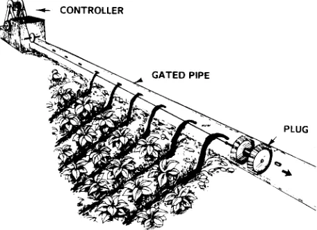
In furrow cablegation, a gated pipe is laid across the upper end of the field on a uniform downward slope. The pipe is sized large enough that it doesn't flow full and the outlets are positioned above the level of the flowing water and left open (fig. 1). A flexible plug inserted in the pipe acts as a dam. Water backs up behind the plug and flows out a number of outlets. Because water pressure decreases with distance upstream of the plug, outlet flow rates also decrease and eventually reach zero, where the water surface drops below the outlet level. The number of flowing outlets depends upon the system flow rate, the pipe size and slope, and the outlet size.
Water pressure pushes the plug through the pipe. Plug movement is constrained by a cable which extends back through the pipe to the inlet box where it is wrapped around a reel. Several types of electric and hydraulic controllers are used to control the reel rotation, and thus the plug movement, at a constant, adjustable rate. As the plug moves, it successively passes outlets which start flowing. Each time a new outlet starts flowing, the water drops below the level of the last outlet which had been flowing
Article was submitted for publication in February 1993; reviewed and approved for publication by the Soil and Water Div. of ASAE in June 1993.
The authors are Thomas J. Trout, Agricultural Engineer, and Dennis C. Kincaid, Soil and Water Management Unit, USDA-Agricultural Research Service, Kimberly, ID.
further back up the pipe. Thus the set of furrows being irrigated moves slowly and constantly across the field.
Furrow cablegation water applications are different from conventional furrow irrigation because the set of furrows being irrigated moves constantly across the field, and flows to each furrow decrease with time. These differences prevent the use of some methods normally used to evaluate furrow irrigation, and present opportunities for simpler evaluation data collection procedures. This article describes furrow evaluation procedures for cablegation systems.
GENERAL CONCEPTS
The goal of irrigation evaluation is to quantify the gross water application to the field, the average infiltrated depth, and the distribution of the infiltrated water throughout the field. By comparing the infiltrated water to the preceding soil water deficit, the deep percolation loss and the various efficiency parameters can be determined (ASAE, 1993).
( 1 ) D – Q '
g P L
sr.) 140
120: Recession
130
180MPlug I
Advance
100 200 300
Distance from Head End (m) 190
0 400
150
0
N,
160
170
Cablegation system evaluations are often carried out to compare their potential and actual efficiencies to those of conventional systems.
Evaluation of conventional furrow irrigation systems requires measuring inflow and runoff rates, and furrow stream advance and possibly recession rates, from a set of furrows (ASAE, 1993). Infiltration rates are determined independently or can be estimated from the measurements using volume balance methods. The measurement procedure is time consuming and inconvenient because observations must be made throughout the irrigation event for a set of furrows which often lasts 12 to 24 h.
Because a cablegation irrigation set moves constantly across the field, time and space are interchangeable. Once a cablegation system reaches steady-state conditions (the plug has been moving for one set width), there are furrows in all stages of the irrigation process (fig. 2). Furrows near the plug are in the advance phase, those further behind (upstream of) the plug are producing runoff, and those near the end of the set, where the flow rates are low, are in recession. Thus, a complete irrigation can be observed either by monitoring one furrow over time, as in conventional evaluation methods, or by observing all furrows at one point in time. The plug movement rate is the transformation that links space and time. This peculiar characteristic allows rapid and efficient data collection. Evaluating complete irrigation sets instead of one or a small group of furrows also reduces the impact of furrow-to-furrow variability on the evaluation results.
EVALUATION PROCEDURES GROSS APPLICATION
Gross application depth, D [m (ft)], is calculated from the system inflow rate, Qi [E/s (ft3 /s)], the plug speed, P [m/h (ft/h)], and the furrow length, L [m (ft)]:
Figure 2–Overhead view of a cablegation irrigation set with the head end of the field at the left and the plug moving downward, showing the initial group of furrows (bottom) in advance, the middle group with completed advance, and the final group in recession (Nm and Nq are the mean and low-quarter number of furrows with water, respectively).
where c is a unit conversion constant of 3.6 (m3/L)•(s/h) in SI units or 3,600 (s/h) in English units. This equation is equivalent to assuming all the flow is concentrated on one furrow at a time.
As with conventional systems, either the system inflow rate or the sum of the flows from the individual outlets (furrow inflows) can be measured. If a meter or weir is not built into the delivery system, measuring outlet flows is often more practical. If the irrigation set is large, every second or third outlet can be measured and the sum adjusted accordingly. Changes over time in the number of outlets flowing indicate fluctuations in the system inflow rate.
Cablegation outlet flow rates (furrow inflow rates) also provide information to help diagnose system installation problems such as non-uniform pipe slope (see Diagnosis section). A plot of the outlet flow rates (fig. 3) also represents the inflow hydrograph for individual furrows if furrow number behind the plug is converted to elapsed time by multiplying by the time interval for the plug to move between outlets, tN (h):
t n = (2)
P
where s is the furrow spacing [m (ft)]. The inflow hydrograph is useful to estimate the soil infiltration function.
RUNOFF PERCENTAGE AND AVERAGE INFILTRATED DEPTH Because furrows are in all stages of irrigation, cablegation tailwater runoff from the field remains fairly constant with time (fig. 4). Thus field runoff can be measured anytime the system is under steady-state conditions. Runoff can be measured with a flume in the tailwater ditch or by summing individual furrow runoff rates measured at one point in time with small flumes (fig. 3). Furrow runoff rates are also useful to estimate furrow infiltration rates and variability. Field runoff rate, Qr [L/s (ft3/s], divided by inflow rate times 100 gives runoff percentage. Inflow rate minus runoff rate divided by
6"
Ir
0
LL
0
LL
180 170 160 150 140 130
Furrow Number
Figure 3–Cablegation furrow inflow and outflow rates showing measured flows and smoothed relationships. The plug is at furrow number 190 (qf is the inflow rate where runoff ceases).
-1.2
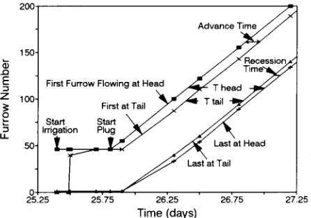
First Furrow Flowing at Head
First at Tail Start Start Irrigation Plug
Advance Time
Recession Time
4,
Last at Head 200
150-E Z 100
2
LL
50-T head T tail
Last at Tail
0
25 25 25.75 26.25 26.75
Time (days)
27 25 40
For example, if water is flowing in 50 furrows at the tail (outflow) end, T at the tail is 50-t
N
. Noting the position (furrow number) of the first flowing outlet (plug position) and the last flowing outlet at the head (inflow) end of the field, and the first and last furrow with runoff at the tail end several times during the irrigation indicates the variability in advance, recession, and T across the field (fig. 5). Identifying the furrow numbers with stakes at the head and tail ends simplifies this process. Because furrow infiltration rates are not uniform, furrow advance and recession times are not uniform, and some judgment may be required to estimate the first and last furrow with runoff."Fri
30-a)
cr
20-0 LT
a)
LL
10-z Inflow
Volume = 13,300 m3
(470,000 tt3)
Runoff
Volume = 2700 m (95,000 ft
0
25 26 27 28 29 300
Time (days)
Figure 4-Field inflow and runoff rate hydrographs.
plug speed and furrow length gives the average infiltrated depth,
Dn
Ern (ft)]:D -
n P•L
c• (Q —
' Q)
(3 )Temporal variations in runoff reflect either spatial variation in field conditions such as infiltration rate, slope, or row length, or variation in the system inflow rate. Runoff measurements over time indicate the amount of spatial variability.
ADVANCE, RECESSION, AND INFILTRATION OPPORTUNITY TIME
Cablegation advance and recession rates can be determined by measuring the advance and recession distances in all furrows at one point in time, rather than the conventional procedure of measuring advance times to preset distances for individual furrows. Advance distances can be quickly measured by a person pacing down the field and noting the paces to the flow front for each furrow. The resulting plot of advance and recession distances (fig. 2) can be converted to advance and recession time curves by transforming furrow numbers to time by multiplying by t
N
(eq. 1). For example, the inflow time for the fifth furrow behind the plug is 5•N
. Because of the gradual inflow decrease with cablegation, recession normally occurs first from the tail end of the furrow and may continue for a significant portion of the irrigation time. Thus, recession is often a more important component of cablegation evaluation than for conventional systems.For most evaluation parameters, complete advance and recession curves are not required. Only the infiltration opportunity time, T, at specified locations along the furrows is sufficient. This is easily determined by counting the number of furrows receiving water at any time at those locations, N, and converting to time by multiplying by the plug advance time interval, t
N
.T=N (4)
INFILTRATION RATE
Because furrow inflow rate decreases with time, the volume balance techniques often used to estimate the furrow infiltration function from advance curves (ASAE, 1993) are not directly applicable to cablegation. If advance is fairly rapid so that inflow rate does not decrease too much during advance, the volume balance method can be used with the average inflow rate during advance to make an estimate of the infiltration function at short opportunity times. However, when average infiltrated depth and advance and recession are measured, infiltration rate at short times is not required to evaluate the irrigation event. Only the infiltration rate near the end of the irrigation, or final infiltration rate, is required to estimate the distribution uniformity of infiltrated water.
The furrow inflow and runoff hydrographs (fig 3) can be used to make estimates of infiltration rate late in the irrigation event. Assuming furrow surface storage is constant late in the irrigation, the difference between furrow inflow and runoff rates near the end of irrigation, Aq
f
[L/s (ft3/s)], divided by the furrow spacing and length, gives the final infiltration rate,If
[m/h (ft/h)] (fig. 3).If-
c Aq
f
s L (5 )
At the time runoff ceases from a furrow and recession begins, only the inflow needs to be measured. If the shape of the inflow hydrograph is known from previous
measurements, this inflow rate can be estimated based on the number of furrows in recession. For example, for the inflow hydrograph shown in figure 3, if three furrows are in recession, the Aq f can be estimated as 0.22 L/s (0.058 ft3/s).
If surface storage is large (small furrow slopes) and gross application is small (fast plug speed), a significant portion of infiltration may derive from decreasing surface storage (resulting from inflow rate decreases) rather than from inflow. This will result in If, calculated only from the inflow rate, underestimating the true value.
A Kostiakov infiltration function can be estimated from the final infiltration rate and average infiltrated depth. The exponent, a, and coefficient, k, are given by:
a= If tf D n
k = Dn t;
where tf (h) is the elapsed time since inflow began when runoff ceases (i.e., number of furrows in advance and with runoff, multiplied by tN). Equations 6 and 7 are derived by simultaneously solving the Kostiakov cumulative infiltration and infiltration rate relationships at time tf. These calculations assume: 1) by time t f, infiltration rate is uniform along the furrow (effects of infiltration opportunity time differences on I f are small); 2) the remaining inflow after recession begins is small relative to the average infiltrated depth; 3) surface storage is small relative to average infiltrated depth; and 4) the rate of change in surface storage at t f is small relative to If. The last two assumptions are often not met in low-sloped furrows with large surface storage.
Corrections can be made to improve the coefficient estimates. For example, the cablegation design computer model (Kincaid, 1992) uses this procedure to estimate furrow infiltration parameters. In the model, the inflow hydrograph is calculated so only gross application, percent runoff, and the number of furrows in recession are required. The model corrects D n for remaining inflow after tf and surface storage at tf, and corrects If for the rate of surface storage change at tf.
DISTRIBUTION UNIFORMITY
The distribution uniformity, DU, is the average depth infiltrated in the low quarter (the quarter of the field area receiving the least water), Dq [m (ft)], divided by average depth infiltrated on the field, D n . If the infiltration capacity is assumed uniform (spatial infiltration variability is ignored), the distribution uniformity can be calculated from infiltration opportunity times. The low-quarter infiltration, Dq, can be estimated from:
D q = D n – I f – T q ) (8)
where T. = the average infiltration opportunity time for the field (h) and Tq = the average infiltration opportunity time for the low quarter (h). With cablegation on sloping,
open-ended furrows, the low quarter is always the tail one-quarter of the field. This calculation assumes If remains constant from T at the tail end of the field to the end of the irrigation, so that the infiltration opportunity time distribution and infiltrated depth distribution are the same. Thus, equation 8 applies best to soils with sustained final infiltration rates and will tend to underestimate Dq and DU when I f is not constant. However, the low estimate of If which results from ignoring surface storage change usually more than compensates and results in a high estimate of D q and DU. The procedure also assumes that infiltration does not vary with furrow wetted perimeter. No consistent infiltration versus wetted perimeter relationship has been determined (Trout, 1992). However, wetted perimeter effects would be expected to lower DU since flow rates and thus wetted perimeter are smaller at the tail end.
The T. and I', values can be calculated from the average numbers of furrows with water at any given time for the whole field length and for the low quarter (N m and Nq , respectively, in fig. 2), times t N . These average numbers of furrows can be determined by subdividing the whole field (for Nm) and the tail quarter (for Nq) into equal length increments, counting the number of furrows with water in each increment, and dividing by the number of increments. The field average infiltration opportunity time (and thus N m) will generally occur between 53% (for relatively constant advance and recession rates) and 60% of the distance from the head end, and Ty (and thus Nu) will occur at about 88% of the distance from the head end. Therefore, only counting the number of furrows with water at those distances from the head end is usually sufficient. The DU can then be calculated as:
DU – q – 1 If (N.– N q ) tN (9) Dn D n
NON-STEADY STATE CONDITIONS
The above procedures apply when the cablegation plug movement rate and the system inflow rate have been constant for at least one set time (the time to advance one set width) and the pipe slope and field conditions (slope, length, and infiltration) are uniform across the set. When steady-state conditions do not apply, the analysis is more difficult and depends on the particular conditions. On fields where the pipe slope or field conditions change, the steady-state procedures should be applied to subsections of the field with uniform conditions. In transition areas, parameter estimates, supported by advance and runoff measurements, must be made.
Non-steady state conditions also occur at field edges where the irrigation begins and ends. Several options are available to initiate and complete cablegation irrigation (Kemper et al., 1987). The recommended cablegation configuration uses a bypass weir and pipe to divert extra flow from the initial to the final set of furrows (Kincaid and Kemper, 1984). This allows the plug to start operating from the first furrow, and the irrigation is finished when it reaches the final furrow. If the system is adjusted properly (correct weir width and crest height), gross application is equal on all furrows and the initial set operates under normal steady-state conditions. However, the final set receives its water in two portions – at the beginning and (6)
(7)
end of the irrigation - and thus advance and recession are different and distribution uniformity is generally lower than for the rest of the field.
A common start-up method if the bypass is not used is to reel out the plug about 2/3 of a normal set width and leave it in position for about 2/3 of a normal set time before releasing it. When the plug reaches the last furrow (end of the pipe), the water is allowed to continue running for about 2/3 of a set time. With this procedure, the downstream portion of the initial set and upstream portion of the final set receive a little more water, and the outside portions of the edge sets (the outside edges of the field) receive a little less water than the rest of the field.
Field inflow and runoff volumes for the complete irrigation (fig. 4) allow field gross application and average infiltrated depth to be calculated and compared to steady-state values. Water distribution on the edge furrows can be estimated with measurements of head and tail infiltration opportunity time on individual furrows.
EXAMPLE
A cablegation irrigation was evaluated on a 340 m (1,100 ft) wide x 400 m (1,300 ft) long field with furrows on 0.76 m (2.5 ft) spacing. The system was started at 9:30 on the 25th with an inflow of 35 L/s (1.23 ft 3/s). As figure 5 shows, the plug was initially reeled out to the 45th furrow and held in place for 9.5 h before being set in motion (no bypass). The plug speed was set at 3.5 m/h (11.5 ft/h) (tN = 0.22 h) in order to give a gross application depth of 0.090 m (0.30 ft) (eq. 1). The plug reached the end of the field (furrow No. 450) at 10:00 on the 29th and was held in place there until the water was shut off at 19:30 so that the last furrows would receive sufficient water.
The first and last furrows with water at the head and tail ends of the field were observed two or three times each day (fig. 5). These data showed that the plug continued to move constantly at the preset rate of 3.5 m/h (11.5 ft/h) and advance and recession times remained fairly constant. Sixty-nine furrows received inflow simultaneously from the system with 11-to-13 furrows in advance and 5-to-7 furrows in recession at all times. Thus average advance and recession times were 2.6 and 1.3 h, respectively, and T at the head and tail ends were 15 and 11 h, respectively (eq. 4).
On the morning of the 27th, when the plug had reached furrow No. 190, furrow inflows and outflows were measured and advance and recession distances were paced. To save time, flows in alternate furrows were measured. The inflow and outflow hydrographs, plotted in figure 3, exhibit typical variability. Summing and doubling the measured inflows and outflows yielded a field inflow rate of 35 L/s (1.23 ft3/s) (as set) and a tailwater runoff rate of 6.6 L/s (0.23 ft 3/s) or 19% of the inflow. Thus, the steady-state average infiltrated depth was (from eq. 3):
3.6 • (35 L/s - 6.6 L/s)
D - - 0.073 m
3.5 m/h • 400 m
3600 •• (1.23 ft3 /s - 0.23 ft3 /s)
D - - 0.24 ft
11.5 ft/h • 1300 m
The furrow inflow rate when the runoff decreased to zero was 0.22 L/s (0.0078 ft3 /s) giving a final infiltration rate of (from eq. 5):
3.6 0.22 L/s
I f = - 0.0026 m/h
0.76 m • 400 m
3600 • 0.0078 ft 3 /s
If = - 0.0086 ft/h
2.5 ft • 1300 ft
The furrow advance and recession distances, plotted in figure 2, showed that the average set width for the field, Nm, was 63 furrows, while the average set width in the low quarter of the field, Nm was 55 furrows. Thus, T m T9 -(63 - 55) - 0.22h) = 1.7 h, and the low quarter application is (from eq. 8):
Dq = 0.073 m - 0.0026 m/h - 1.7 h = 0.069 m
Dq = 0.24 ft - 0.0086 ft/ h • 1.7 h= 0.23 ft
or 0.004 m (0.01 ft) less than the average infiltrated depth. The distribution uniformity is (from eq. 9):
1 - 0.0026 m/h - (63 - 55) • 0.22 h _ 0.94 DU
-0.073 m
0.0086 ft/ h (63 - 55) • 0.22 h _ 0.94 DU
-0.24 ft
A volume balance computer cablegation model (Kincaid, 1992) applied to the measured conditions predicted a DU of 0.91. The difference is the result of assuming the final infiltration rate and surface storage were constant.
Field inflow rates were checked periodically and runoff was continuously recorded with a flume and data logger. The inflow hydrograph (fig. 4) showed that actual gross application was 13 300 m 3 (470,000 ft 3 ) or 0.098-m (0.32-ft) depth. The excess beyond the 0.090-m (0.30-ft) steady-state gross application was due to the extra 9.5 h of application time at the end of the irrigation. The runoff hydrograph showed higher runoff rates at the beginning and the ends of the irrigation when the plug was stationary. This higher runoff more than compensated for the initial 3 h with no runoff so that field runoff was 20% of inflow (compared to 19% steady-state runoff). The field average infiltrated depth was 13 300 m 3 - 2700 m3 = 10 600 m 3 (370,000 ft3) = 0.078 m (0.26 ft) or only 0.005 m (0.02 ft) larger than that under steady-state conditions. Since this extra was applied to the initial 45 and final 69 furrows, the average infiltration depth to those furrows was 0.088 m (0.29 ft) or 20% greater than to the rest of the field.
PROBLEM DIAGNOSIS
High Runoff Rates. With the cutback application of
cablegation, runoff should not exceed 30%, and less than 20% runoff is usually achievable. On soils with sustained final infiltration rates, reduce outlet sizes (gate settings) to reduce furrow inflow rates. This increases irrigation time without increasing gross application. On soils with rapidly decreasing infiltration rates (small Kostiakov exponent), inflow rates have little effect on average infiltrated depth and thus total runoff, so reduce the gross application by increasing plug speed.
Low DU Due to Slow Advance. With the cablegation
cutback application, advance rates should generally be faster than with conventional systems. Increase inflow rates by increasing outlet sizes.
Low DU Due to Long Tail-end Recession. Tail-end
recession can be a problem with cablegation on soils with sustained infiltration rates. The volume of inflow (sum of furrow inflows) plus surface storage after recession begins quantifies the problem. Decrease the system inflow to reduce the number of furrows with low flow (shorten the tail of the inflow hydrograph). Use siphoning outlets (Kemper et al., 1987) which cut off the outlet flow below a minimum flow rate.
Variation in Outlet Flow Rates. Because cablegation
pipe is installed on a precise slope and outlets can be preset at a uniform opening and left open, furrow-to-furrow inflow volumes should be more uniform than with conventional gated-pipe systems. Inflow volume coefficients of variation below 5% are achievable (compared to 15 to 25% measured on typical conventional systems) (Trout and Mackey, 1988). If inflow variations from the hydrograph curve are random, use a gauge or jig to set the outlet openings more uniformly. If variations show trends over several furrows, survey and regrade the cablegation pipe (high flow rates and relatively longer outlet flow times indicate relatively low outlets while low flow rates and short flow times indicate high outlets).
Variation in Runoff Rates. Assuming inflows are
uniform, variations in advance times and deviations of furrow runoff from the runoff hydrograph (fig. 3) indicate furrow-to-furrow infiltration variability. A repeated variation pattern usually indicates uneven wheel compaction of furrows. Gradual trends indicate soil variations across a field. Differentially adjust pipe outlets to make runoff more uniform. Since cablegation outlets are left open, these adjustments can be retained from irrigation-to-irrigation. Outlet adjustment over a short spatial range (i.e., to correct uneven wheel packing), does not improve infiltration uniformity. Adjustment of groups of outlets to correct runoff trends improves infiltration uniformity. For example, reducing outlet size to decrease inflow and runoff does not change gross application but increases irrigation times (increases the set width) to compensate for the lower infiltration rate.
Edge Effects Significantly Reduce Uniformity.
Improve system operational start-up and completion procedures or install a bypass system. Edge effects are relatively more important on narrow fields, so cablegation generally should not be used on fields which are irrigated in less than four set widths. Reduce the system inflow to narrow the set width. Subdividing water supply between fields is not necessarily a disadvantage with automated systems.
SUMMARY
The constant movement of cablegation sets allows simple evaluation data collection procedures. An approximately two-hour field visit by two technicians during which furrow inflow and runoff hydrographs, advance and recession distances, and plug movement speed are measured can produce close approximations of gross application, average infiltrated depth, runoff, and distribution uniformity under steady-state conditions. This information can be used to help achieve the high potential application efficiency of the system.
REFERENCES
ASAE Standards, 40th Ed. 1993. EP419. Evaluation of furrow irrigation systems. St. Joseph, MI: ASAE.
Kemper, W. D., W. H. Heinemann, D. C. Kincaid and R. V. Worstell. 1981. Cablegation: 1. Cable controlled plugs in perforated supply pipes for automatic furrow irrigation. Transactions of the ASAE 24(6):1526-1532.
Kemper, W. D., D. C. Kincaid, R. C. Worstell, W. H. Heinemann, T. J. Trout and J. E. Chapman. 1985. Cablegation systems for irrigation: Description, design, installation, and performance. USDA-ARS No. 21, Kimberly, ID.
Kemper, W. D., T. J. Trout and D. C. Kincaid. 1987. Cablegation: Automated supply for surface irrigation. In Advances in Irrigation, ed. D. Hillel, 4:1-66. Orlando, FL: Academic Press. Kincaid, D. C. 1992. Cablegation Model. (A computer model to
design furrow cablegation systems for PC compatible computers). Available from USDA-ARS, Kimberly, ID. Kincaid, D. C. and W. D. Kemper. 1984. Cablegation IV. The
bypass method and cutoff outlets to improve water distribution. Transactions of the ASAE 27(3):762-768.
Trout, T. J. 1992. Flow velocity and wetted perimeter effects on furrow infiltration. Transactions of the ASAE 35(3):855-863. Trout, T. J. and D. C. Kincaid. 1989. Border cablegation system
design. Transactions of the ASAE 32(4): 1185-1192. Trout, T. J. and B. E. Mackey. 1988. Furrow inflow and
infiltration variability. Transactions of the ASAE 31(2):531-537.
Trout, T. J., D. C. Kincaid and W. D. Kemper. 1990. Cablegation: a review of the past decade and prospects for the next. In Visions of the Future. Proceedings of the Third National Irrigation Symposium, 21-27. St. Joseph, MI: ASAE.