Gene selection for cancer classification with the help of bees

R E S E A R C H

Open Access

Gene selection for cancer classification

with the help of bees

Johra Muhammad Moosa

, Rameen Shakur

, Mohammad Kaykobad

and Mohammad Sohel Rahman

FromIEEE International Conference on Bioinformatics and Biomedicine 2015 Washington, DC, USA. 9-12 November 2015

Abstract

Background: Development of biologically relevant models from gene expression data notably, microarray data has

become a topic of great interest in the field of bioinformatics and clinical genetics and oncology. Only a small number of gene expression data compared to the total number of genes explored possess a significant correlation with a certain phenotype. Gene selection enables researchers to obtain substantial insight into the genetic nature of the disease and the mechanisms responsible for it. Besides improvement of the performance of cancer classification, it can also cut down the time and cost of medical diagnoses.

Methods: This study presents a modified Artificial Bee Colony Algorithm (ABC) to select minimum number of genes

that are deemed to be significant for cancer along with improvement of predictive accuracy. The search equation of ABC is believed to be good at exploration but poor at exploitation. To overcome this limitation we have modified the ABC algorithm by incorporating the concept of pheromones which is one of the major components of Ant Colony Optimization (ACO) algorithm and a new operation in which successive bees communicate to share their findings.

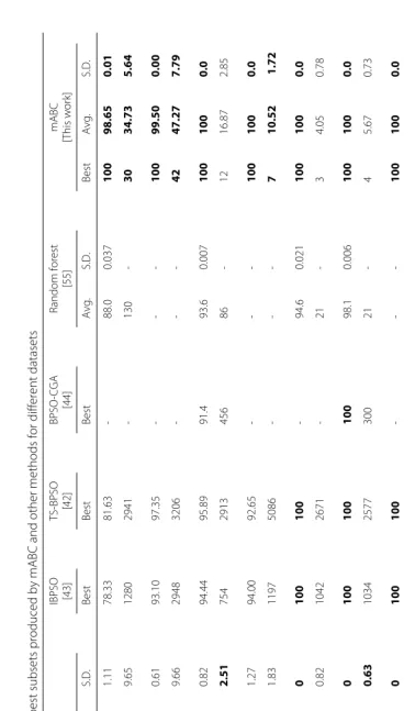
Results: The proposed algorithm is evaluated using a suite of ten publicly available datasets after the parameters are

tuned scientifically with one of the datasets. Obtained results are compared to other works that used the same datasets. The performance of the proposed method is proved to be superior.

Conclusion: The method presented in this paper can provide subset of genes leading to more accurate classification

results while the number of selected genes is smaller. Additionally, the proposed modified Artificial Bee Colony Algorithm could conceivably be applied to problems in other areas as well.

Keywords: Gene selection, Microarray, Cancer classification, Artificial bee colony algorithm, Evolutionary algorithm

Background

Gene expression studies have paved the way for a more comprehensive understanding of the transcriptional dynamics afflicted on a cell under different biological stresses [1–4]. The application of microarrays as a robust and amenable system to record transcriptional profiles across a range of differing species has been growing expo-nentially. In particular, the evaluation of human expres-sion profiles in both health and in disease has implications for the development of clinical bio-markers for diagnosis as well as prognosis. Hence, diagnostic models from gene

*Correspondence: [email protected]

1AEDA Group, Department of CSE, BUET, Dhaka-1205, Dhaka, Bangladesh Full list of author information is available at the end of the article

expression data provide more accurate, resource efficient, and repeatable diagnosis than the traditional histopathol-ogy [5]. Indeed, microarray data is now being used in clinical applications as it is possible to predict the treat-ment of human diseases by analyzing gene expression data [2, 6–9]. However, one of the inherent issues with gene expression profiles are their characteristically high-dimensional noise, contributing to possible high false pos-itive rates. This is further compounded during analysis of such data whereby the use of all genes may poten-tially hinder the classifier performance by masking the contribution of the relevant genes [10–15]. This has led to a critical need for the development of analytical tools and methodologies which are able to select a small subset

of genes both from a practical and qualitative perspec-tive. As a result the selection of discriminatory genes is essential to improve the accuracy and also to decrease the computational time and cost [16].

The classification of gene expression samples involves feature selection and classifier design. However, noisy, irrelevant, and misleading attributes make the classifica-tion task complicated, given they can contain erroneous correlations. A reliable selection method of relevant genes for sample classification is needed in order to increase classification accuracy and to avoid incomprehensibility. The task of gene selection is known as feature selection in artificial intelligence domain. Feature selection has class-labeled data and attempts to determine which features best distinguish among the classes. The genes are consid-ered to be the features that describe the cell. The goal is to select a minimum subset of features that achieves max-imum classification performance and to discard the fea-tures having little or no effect. These selected feafea-tures can then be used to classify unknown data. Feature selection can thus be considered as a principle pre-processing tool when solving classification problems [17, 18]. Theoreti-cally, feature selection problems are NP-hard. Performing an extensive search is impossible as the computational time and cost would be excessive [19].

Gene selection methods can be divided into two cate-gories [20]: filter methods, and wrapper or hybrid meth-ods. Detail review on gene selection methods can be found in [20–25]. A gene selection method is categorized as a filter method if it is carried out independently from a clas-sification procedure. In filter approach instead of search-ing the feature space, selection is done based on statistical properties. Due to lower computational time and cost most previous gene selection techniques in the early era of microarrays analysis have used the filter method. Many fil-ters provide a feature ranking rather than an explicit best feature subset. The top ranking features are chosen man-ually or via cross-validation [26–28] while the remaining low ranking features are eliminated. Bayesian Network [29], t-test [30], Information Gain (IG) and Signal-to-Noise-Ratio (SNR) [5, 31], Euclidean Distance [32, 33], etc. are the examples of filter methods that are usually consid-ered as individual gene-ranking methods. Filter methods generally rely on a relevance measure to assess the impor-tance of genes from the data, ignoring the effects of the selected feature subset on the performance of the classi-fier. This may however result in the inclusion of irrelevant and noisy genes in a gene subset. Research shows that, rather than acting independently, genes in a cell interact with one another to complete certain biological processes or to implement certain molecular functions [34].

While the filter methods handle the identification of genes independently, a wrapper or hybrid method on the other hand, implements a gene selection method merging

with a classification algorithm. In the wrapper methods [35] a search is conducted in the space of genes, evaluating the fitness of each found gene subset. Fitness is deter-mined by training the specific classifier to be used only with the found gene subset and then approximating the accuracy percentage of the classifier. The hybrid methods usually obtain better predictive accuracy estimation than the filter methods [36–39], since the genes are selected by considering and optimizing the correlations among genes. Therefore, several hybrid methods have been imple-mented to select informative genes for binary and multi-class cancer multi-classification in recent times [37, 40–50]. However, its computational cost must be taken into account [39]. Notably, filter methods have also been used as a preprocessing step for wrapper methods, allowing a wrapper to be used on larger problem instances.

genes for some of the datasets. But the number of itera-tions to achieve the target accuracy is higher than ours, which will be reported in the Results and discussion Section of this paper. A simple modified ant colony opti-mization (ACO) algorithm is proposed by Yu et al. in [53], which associates two pheromone components with each gene rather than a single one as follows. One component determines the effect of selecting the gene whether the other determines the effect of not selecting it. The algo-rithm is evaluated using five datasets. It is able to select small number of genes and accuracy is also reasonable. Random forest algorithm for classifying microarray data [54] has obtained good accuracy for some datasets but not for all. Notably, the number of selected genes by the ran-dom forest classification algorithm in [54] has been found to be high for some of the datasets. A new variable impor-tance measure based on the difference of proximity matrix has been proposed for gene selection using random for-est classification by Zhou et al. [55]. Although it fails to achieve the highest accuracy for any dataset, their algo-rithm is able to select small number of genes and achieve satisfactory accuracy for all the datasets. Recently, Deb-nath and Kurita [56] have proposed an evolutionary SVM classifier that adds features in each generation according to the error-bound values for the SVM classifier and fre-quency of occurrence of the gene features to produce a subset of potentially informative genes.

In this paper, we propose a modified artificial bee colony algorithm to select genes for cancer classification. The Artificial Bee Colony (ABC) algorithm [57], proposed by Karaboga in 2005, is one of the most recent swarm intel-ligence based optimization technique, which simulates the foraging behavior of a honey bee swarm. The search equation of ABC is reported to be good at exploration but poor at exploitation [58, 59]. To overcome this limitation we have modified the ABC algorithm by incorporating the concept of pheromone which is one of the major components of the Ant Colony Optimization (ACO) algo-rithm [60, 61] and a new operation in which successive bees communicate to share their results. Even though researchers are unable to establish whether such a com-munication indeed involve information transfer or not, it is known that foraging decisions of outgoing workers, and the probability to find a recently-discovered food source, are influenced by the interactions [62–67]. Indeed, there is a notable proof that for harvester ants, management of foraging activity is guided by ant encounters [68–71]. Even the mere instance of an encounter may provide some information, such as, the magnitude of the colony’s forag-ing activity, and may therefore influence the probability of food collection by ants [72–74].

We believe that the selection of genes by our system provide us some interesting clue towards the importance and contribution of that set of particular genes for the

respective cancer disease. To elaborate, our system has identified that for diffuse large B-cell lymphoma (DLBCL) only three (3) genes are informative enough to decide about the cancer. Now, this could turn out to be a string statement with regards to the set of genes identified for a particular cancer and we believe further biological valida-tion is required before making such a string claim. We do plan to work towards validation of these inferences.

During the last decade, several algorithms have been developed depending on different intelligent behaviors of honey bee swarms [57, 75–85]. Among those, ABC is the one which has been most widely studied on and applied to solve the real world problems, so far. Compre-hensive study on ABC and other bee swarm algorithms can be found in [86–89]. The algorithm has the advan-tage of sheer simplicity, high flexibility, fast convergence, and strong robustness which can be can be used for solv-ing multidimensional and multimodal optimization prob-lems [90–92]. Since the ABC algorithm was proposed in 2005, it has been applied in many research fields, such as flow shop scheduling problem [93, 94], parallel machines scheduling problem [95], knapsack problem [96], travel-ing salesman problem [97], quadratic minimum spanntravel-ing tree problem [98], multiobjective optimization [99, 100], generalized assignment problem [101], neural network training [102], and synthesis [103], data clustering [104], image processing [105], MR brain image classification [106], coupled ladder network [107], wireless sensor net-work [108], vehicle routing [109], nurse rostering [110], computer intrusion detection [111], live virtual machine migration [112], etc. Studies [86, 113] have indicated that ABC algorithms have high search capability to find good solutions efficiently. Besides, excellent performances has been reported by ABC for a considerable number of prob-lems [98, 100, 114]. Karaboga and Basturk [113] tested for five multidimensional numerical benchmark functions and compared the ABC performance with that of Differ-ential Evolution (DE), Particle Swarm Optimization (PSO) and Evolutionary Algorithm (EA). The study concluded that ABC gets out of a local minimum more efficiently for multivariable and multimodal function optimization and outperformed DE, PSO and EA.

better solutions. The exploration ability and the exploita-tion ability contradict to each other, so that the two abilities should be well balanced to achieve good per-formance on optimization problems. As a result, several improvements of ABC have been proposed over the time. Baykasoglu et al. [101] incorporated the ABC algorithm with shift neighborhood searches and greedy randomized adaptive search heuristic and applied it to the generalized assignment problem. Pan et al. [93] proposed a Discrete Artificial Bee Colony (DABC) algorithm with a variant of iterated greedy algorithm with total weighted earli-ness and tardiearli-ness penalties criterion. Li et al. [116] used a hybrid Pareto-based ABC algorithm to solve flexible job shop-scheduling problems. In the proposed algorithm, each food sources is represented by two vectors, the machine assignment and the operation scheduling. Wu et al. [117] combined Harmony Search (HS) and the ABC algorithm to construct a hybrid algorithm. Comparison results show that the hybrid algorithm outperforms ABC, HS, and other heuristic algorithms. Kang et al. [118] antic-ipated a Hooke Jeeves Artificial Bee Colony algorithm (HJABC) for numerical optimization. HJABC integrates a new local search named ‘modus operandi’ which is based on Hooke Jeeves method (HJ) [119] with the basic ABC. Opposition Based Lévy Flight ABC is developed by Sharma et al. [120]. Lévy flight based random walk local search is proposed and incorporated with ABC to find the global optima. Szeto et al. [109] proposed an enhanced ABC algorithm. The performance of the new approach is tested on two sets of standard benchmark instances. Sim-ulation results show that the newly proposed algorithm outperforms the original ABC and several other existing algorithms. Chaotic Search ABC (CABC) is introduced by Yan et al. [121] to solve the premature convergence issue of ABC by increasing the number of scout and rational using of the global optimal value and chaotic Search. Again a Scaled Chaotic ABC (SCABC) method is proposed in [106] based on fitness scaling strategy and chaotic theory. Based on the Rossler attractor of chaotic theory a novel Chaotic Artificial Bee Colony (CABC) is developed in [122] to improve the performance of ABC. An Improved Artificial Bee Colony (IABC) algorithm is proposed in [123] to improve the optimization ability of ABC. The paper introduces an improved solution search equation in employee and scout bee phase using the best and the worst individual of the population. In addition, the initial population is generated by the piecewise logis-tic equation which employs chaologis-tic systems to enhance the global convergence. Inspired by Differential Evolu-tion (DE), Gao et al. [124] proposed an improved soluEvolu-tion search equation. In order to balance the exploration of the solution search equation of ABC and the exploitation of the proposed solution search equation, a selective prob-ability is introduced. In addition, to enhance the global

approach named PS-ABC is introduced by Xu et al. [112]. The method utilizes the binary search idea and the Boltz-mann selection policy to achieve the uniform random ini-tialization and thus to make the whole PSABC approach have a better global search potential and capacity at the very beginning. To obtain more efficient food positions Sharma et al. [130] introduced two new mechanisms for the movements of scout bees. In the first method, the scout bee follows a non-linear (quadratic) interpolated path while in the second one, scout bee follows Gaussian movement. The first variant is named as QABC, while the second variant is named as GABC. Numerical results and statistical analysis of benchmark unconstrained, con-strained and real life engineering design problems indicate that the proposed modifications enhance the performance of ABC. In order to improve exploitation capability of ABC a new search pattern is proposed by Xu et al. [131] for both employed and onlooker bees. In the new approach, some best solutions are utilized to accelerate the convergence speed. A solution pool is constructed by storing some best solutions of the current swarm. New candidate solutions are generated by searching the neigh-borhood of solutions randomly chosen from the solution pool. Kumar et al. [97] added crossover operators to the ABC as the operators have a better exploration property. Ji et al. [96] developed a new ABC algorithm combining chemical communication way and behavior communica-tion way based on researches of entomologists. The new ABC algorithm introduces a novel communication mech-anism among bees. In order to have a better coverage and a faster convergence speed, a modified ABC algo-rithm introducing forgetting and neighbor factor (FNF) in the onlooker bee phase and backward learning in the scout bee phase is proposed by Yu et al. [108]. Bansal et al. [132] introduced Memetic ABC (MeABC) in order to balance between diversity and convergence capability of the ABC. A new local search phase is integrated with the basic ABC to exploit the search space identified by the best individual in the swarm. In the proposed phase, ABC works as a local search algorithm in which, the step size that is required to update the best solution, is con-trolled by Golden Section Search (GSS) [133] approach. In the memetic search phase new solutions are gener-ated in the neighborhood of the best solution depending upon a newly introduced parameter, perturbation rate. Kumar et al. [134] also proposed memetic search strat-egy to be used in place of employed bee and onlooker bee phase. Crossover operator is applied to two randomly selected parents from current swarm. After crossover operation two new offspring are generated. The worst par-ent is replaced by the best offspring, other parpar-ent remains same. The experimental result shows that the proposed algorithm performs better than the basic ABC without crossover in terms of efficiency and accuracy. Improved

onlooker bee phase with help of a local search strategy inspired by memetic algorithm to balance the diversity and convergence capability of the ABC is proposed by Kumar et al. [135]. The proposed algorithm is named as Improved Onlooker Bee Phase in ABC (IOABC). The onlooker bee phase is improved by introducing modified GSS [133] process. Proposed algorithm modifies search range of GSS process and solution update equation in order to balance intensification and diversification of local search space. Rodriguez et al. [95] combined two signifi-cant elements with the basic scheme. Firstly, after produc-ing neighborproduc-ing food sources (in both the employed and onlooker bees phases), a local search is applied with a pre-defined probability to further improve the quality of the solutions. Secondly, a new neighborhood operator based on the iterated greedy constructive-destructive procedure [136, 137] is proposed. For further discussion please refer to the available reviews on ABC [138]. Several algorithms have been introduced that incorporates idea of ACO or PSO in bee swarm based algorithms. But our approach is unique and different from others. Hybrid Ant Bee Colony Algorithm (HABC) [139] considers pheromone for each candidate solution. On the other hand we incor-porated pheromone for each gene (solution components). Our approach to find neighboring solution is different from basic ABC. But HABC follows the same neighbor production mechanism as basic ABC. In our algorithm pheromone deposition is done after each bee stage. While selecting a potential candidate solution we depend on its fitness, but HABC selects a candidate depending upon its pheromone value. Most importantly in our algorithm scout bees make use of the pheromone while exploring to find new food source. Ji et al. [96] proposed an arti-ficial bee colony algorithm merged with pheromone. In this paper scouts are guided by pheromone along with some heuristic information while we only make use of pheromone. The paper updates pheromone only in the employed bee stage while we update pheromone in all the bee stages. Pheromone laying is done by depositing a pre-defined constant amount. But amount of pheromone we have deposited is a function of fitness measures. Kefayat et al. [140] proposed a hybrid of ABC and ACO. Inside loop contains the ABC and outside loop is ACO with-out any modification. ABC is applied in the inner loop to optimize a certain constraint (source size) for each ant. Zhu et al. [115] uses ABC in a problem with continuous space. We indirectly guide scout through the best found solutions whether this paper guides the employed and onlooker bees.

Methods

However, in comparison to the number of genes involved which often exceeds several thousands, available training datasets generally have a fairly small sample size for clas-sification. Hence, inclusion of redundant genes decreases the quality of classification thus increasing false positive rates. To overcome this problem one of the approaches in practice is to search for the informative genes along with applying a filter beforehand. Use of confidently pre-filtering makes it possible to get rid of the majority of redundant noisy genes. Consequently, the underlying method to search the informative genes becomes easier and efficient with respect to time and cost. Finally, to eval-uate the fitness of the selected gene subset a classifier is utilized. The selected genes are used as features to classify the testing samples. The inputs and outputs of the method are:

• Input:G= {G1,G2,. . .,Gn}, a vector of vectors,

wheren is the number of genes and

Gi= {gi,1,gi,2,. . .,gi,N}is a vector of gene expressions

for theithgene whereN is the sample size. So,gi,jis

the expression level of theithgene in thejthsample.

• Output:R= {R1,R2,. . .,Rm}, the indices of the

genes selected in the optimal subset. Wherem is the

selected gene size.

The gene selection method starts with a preprocessing step followed by a gene selection algorithm. Finally the classification is done. In what follows, we will describe these steps in detail.

Preprocessing

To make the experimental data suitable for our algorithm and to help the algorithm run faster the preprocessing step is incorporated. The preprocessing step contains the following two stages:

• Normalization

• Prefilter

Normalization Normalizing the data ensures the alloca-tion of equal weight to each variable by the fitness mea-sure. Without normalization, the variable with the largest scale will dominate the fitness measure [141]. Therefore, normalization reduces the training error, thereby prov-ing the accuracy for the classification problem [142]. The expression levels for each gene are normalized at this step to [0, 1] using the standard procedure which is shown in Eq. 1 below.

x=lower+

upper−lower× value−value_min

value_max−value_min

(1)

Here, among all the expression levels of the gene in consideration,value_maxis the maximum original value,

value_minis the minimum original value,upper (lower)

is 1 (0) andx is the normalized expression level. So for all gene after normalization, value_max will be 1 and

value_minwill be 0.

Prefilter Gene expression data are characteristically multi faceted given the inherent biological complexity such networks reside in. The huge number of genes causes great computational complexity in wrapper meth-ods when searching for significant genes. Before applying other search methods it is thus prudent to reduce gene subset space by pre-selecting a smaller number of infor-mative genes based on some filtering criteria. Several filter methods have been proposed in the literature which can be used to preprocess data. These include Signal-to-Noise Ratio (SNR) and Information Gain (IG) [5, 31],t-test [30], Bayesian Network [29], Kruskal-Wallis non-parametric

analysis of variance (ANOVA) algorithm [143–145], F

-test (ratio of in between group variance to within group variance) [146, 147], BW ratio [148], Euclidean Distance [32, 33], etc. After the prefilter stage, we get a ranking of the genes based on the applied statistical methods.

Because of the nature of gene expression data the selected statistical method should be able to deal with high dimensional small sample sized data. According to the assumption of the data characteristics two types of filtering methods exist, namely, parametric and non parametric. Both types of filtering techniques have been employed individually in our proposed algorithm for the sake of comparison. Among many alternatives, in our work, Kruskal Wallis [143–145] andF-test [146, 147] are employed individually to rank the genes. Notably, the former is a non parametric method and the latter is a parametric one.

because it does not require strong distributional assump-tions [154], it works well on small samples [155], it is suited for multiclass problems, and its p-values can be calculated analytically. The Kruskal-Wallis test is utilized to determinep-values of each gene. The genes are then sorted in increasing order of thep-values. The lower thep -value of a gene, the higher the rank of the gene. The steps of the Kruskal-Wallis test are given below:

Step 1 For each gene expression vectorGi,

Step 1.a We rank all gene expression levels across all classes. We Assign any tied values the average of the ranks they would have received if they had not been tied.

Step 1.b We calculate the test statisticsKifor gene

expression vectorGiof theithgene, which is

given by Eq. 2 below:

Ki=

12

N(N+1)

Ci

k=1

ni_k

¯

r_ki − (N+1)

2

2

(2)

Here, for theith_gene,

N is the sample size,

Ciis the number of different classes,

ni_kis the number of expression levels that are

from classk, and

¯

ri_kis the mean of the ranks of all expression

level measurements for classk.

Step 1.c If ties are found while ranking data in theith

gene, correction of ties must be done. For

this correction,Kiis divided by:

(1−

_Ti

j=1t3j−tj

N3_−N ), whereTiis the number of

groups of different tied ranks for theithgene

andtjis the number of ties within groupj.

Step 1.d Finally thep-value for theith_gene,p

iis

approximated byPr(χ_C2

i−1≥Ki), where

χ2

Ci−1refers to the critical chi-square value.

To compute thep-values, necessary

functions of the already implemented package from https://svn.win.tue.nl/trac/ prom/browser/Packages/Timestamps/ Trunk/src/edu/northwestern/at/utils/math/ are incorporated in our method.

Step 2 After thep-values for all the genes are calculated,

we rank each geneGiaccording topi. The lower

thep-value of a gene, the higher is its ranking.

Kruskal-Wallis is used as a preprocessing step in many gene selection algorithms [156–158]. Kruskal-Wallis test is utilized to rank and pre-select genes in the two-stage gene selection algorithm proposed by Duncan et al. [158].

In the proposed method the number of genes selected from the ranked genes is optimized by cross-validation on the training set. Wang et al. [157] applied Kruskal-Wallis rank sum test to rank all the genes for gene reduction. Obtained results from their study indicate that gene rank-ing with Kruskal-Wallis rank sum test is very effective. To select an initial informative subset of tumor related genes Kruskal-Wallis rank sum test is utilized by Wang et al. [156].

Besides applying Kruskal-Wallis in prefiltering stage the use of the algorithm for gene selection is also well stud-ied [159, 160]. Chen et al. [160] studstud-ied application of different test statistics including Kruskal-Wallis for gene selection. Lan et al. [159] applied Kruskal-Wallis to rank the genes. Finally the top ranked genes are selected as features for the target task classifier. The proposed filter is claimed to be suitable as a preprocessing step for an arbitrary classification algorithm.

Like many other non-parametric tests Kruskal-Wallis uses data rank rather than raw values to calculate the statistic. However, by ranking the data some information about the magnitude of differences between scores is lost. For this reason a parametric method called F-test has been applied separately from Kruskal-Wallis to prefilter the genes. Notably, replacing original scores with ranks does not naturally lead to performance reduction; it rather can result in a better performance at best and a slight degradation at worst.

F-test Another approach to identify the genes that are correlated to the target classes from gene expression data is by using theF-test [146, 147].F-test is one of the most widely used supervised feature selection methods. The key idea is to find a subset of features, such that the dis-tances between the data points in different classes are as large as possible, while the distances between the data points in the same class are as small as possible in the data space spanned by the selected features. It uses

vari-ations amongmeans to estimate variations among

indi-vidual measurements.F-score for a gene is the ratio of in between group variance to within group variance, where each class label forms a group. The steps to compute the

F-score are given below:

Step 1 For each gene expression vectorGi, we compute

the Fisher score (i.e.,F -Score). The fisher score

for theithgene is given by Eq. 3 below.

Fi=

Ci

k=1nik(μik−μi)2 Ci

k=1nik(σki)2

(3)

Here for theith_gene,

μi_{is the mean for all the gene expression levels}

μi

kandσkiare mean and standard deviation of the

kthclass respectively,

Ciis the number of classes, and

ni_kis the number of samples associated with the

kthclass.

Step 2 After computing the Fisher score for each genes,

genes are sorted according to theF - score. The

higher theF -score of a gene, the higher is its rank.

F-test has been proved to be effective for determin-ing the discriminative power of genes [161]. Use ofF-test either as a sidekick in gene selection [158, 162] or as a stand-alone gene selection tool [163] both are practiced in the literature. Duncan et al. [158] used F-test as one of the ranking schemes to preselect the genes. Guo et al. [163] proposed a privacy preserving algorithm for gene selection usingF-criterion. The proposed method can be used in other feature selection problems. Au et al. [162] implementedF-test as a criterion function in their pro-posed algorithm to solve the problem of gene selection. Cai et al. [164] pre-selected top 1,000 genes from each dataset according to Fisher’s ratio. To guide the search their method evaluated discriminative power of features independently according to Fisher criterion. Salem et al. [165] reduced the total number of genes in the input dataset to a smaller subset usingF-score.

TheF-score is computed independently for each gene, which may lead to a suboptimal subset of features. Gen-erally, theF-test is sensitive to non-normality [166, 167]. Thus the preferred test to use with microarray data is the Kruskal-Wallis test rather than theF-test since the para-metricity assumption of data distribution often does not hold for gene expression data [153].

Pre-selection of genes The top ranked genes will enter the next phase. After the genes are ranked according to the statistical method in use, we need to calculate the number of genes to nominate for the next stage. There could be two ways to determine the number of genes to be selected in this stage.

Select according top In this approach we predetermine a threshold and select all the genes that have statistics calculated by Kruskal-Wallis (F-test) below (above) the threshold. This approach generally tends to select comparatively large number of genes [157]. To determine a suitable threshold value we have con-ducted scientific parameter tuning in the range of [0, 1]. The analysis is presented in the Additional file 1.

Select according ton Another approach is to select a predetermined number of top ranked genes. The number of genes selected from the ranked genes can be either fixed or optimized by cross-validation on

the training set. EPSO [37] empirically determined a fixed number (500) and used it for all the datasets. Also several other works in the literature used this approach to preselect genes [41, 53, 156, 158, 168]. Li et al. [41] selected 40 top genes with the highest scores as the crude gene subset using Wilcoxon sum rank test. Yu et al. [53] presented detail information about top 10 marker genes. Initially Wang et al. [156] selected 300 top-ranked genes by KWRST. Duncan et al. [158] considered a set of values for number of top-ranked genes. Based on Fisher’s ratio top 1000 genes are selected by Zhou et al. [168]. But the prob-lem in this approach is that different datasets have different sizes. So a fixed value might not be optimal for all the datasets. Determining a value that is good for all the datasets is not possible. So in this article we have selected a percentage of top ranked genes. As a result number of genes selected will depend on the original size of the dataset. Therefore, when the percentage is set to 0.1, only the top 10 % from the ranked genes are supplied to the next stage. We have scientifically tuned the parameter in the range of [0, 1]. The analysis is presented in the Additional file 1.

Gene selection

After the preprocessing step only the most informative genes are left. Now they are fed to the search method to further select a smaller subset of informative genes. In this paper as the search method we have used the modi-fied artificial bee colony (mABC) algorithm as described below.

Artificial Bee Colony The Artificial Bee Colony (ABC) algorithm is one of the most recent nature inspired opti-mization algorithms based on the intelligent foraging behavior of honey bee swarm. ABC algorithm has been proposed by Karaboga in [57] and further developed in [113]. Excellent performances have been exhibited by the ABC algorithm for a considerable number of problems [90–92, 98, 100, 114].

new food source, it becomes an employed bee again. Every scout is an explorer who does not have any guidance while looking for a new food, i.e., a scout may find any kind of food sources. Therefore, sometimes a scout might acci-dentally discover a more rich and entirely unknown food source.

The position of a food source is a possible solution to the optimization problem and the nectar amount of the food source represents the quality of the solution. The bees act as operators over the food sources trying to find the best one among them. Artificial bees attempt to discover the food sources with high nectar amount and finally the one with the highest nectar amount. The onlookers and employed bees carry out the exploitation process in the search space and the scouts control the exploration pro-cess. The colony consists of equal number of employed bees and onlooker bees. In the basic form, the num-ber of employed bees is equal to the numnum-ber of food sources (solutions) thus each employed bee is associated with one and only one food source. For further discus-sion please refer to the available reviews on ABC [138]. The pseudo-code of the ABC algorithm is presented in Algorithm 1.

Algorithm 1:Artificial Bee Colony Algorithm

1 initialize population 2 repeat

3 send the employed bees onto the food sources

and evaluate their fitness (nectar amounts)

4 foreach employed beesdo

5 produce a new solution and determine its

fitness

6 apply greedy selection between new solution

and current solution

7 end

8 evaluate the probability values of the food sources

9 foreach onlooker beesdo

10 select a food source depending on their

fitness

11 produce a new solution and calculate its

fitness

12 apply greedy selection between new solution

and current solution

13 end

14 abandon a position if the food source is

exhausted by the bees

15 send the scout bees to the solution space for

discovering new food sources randomly for the abandoned positions

16 memorize the best food source found so far

17 untilthe stopping criteria are met;

Modified ABC algorithm The search equation of ABC is reported to be good at exploration but poor at exploita-tion [59]. As a result, several improvements of ABC have been proposed over the time [96, 97, 106, 108, 111, 112, 120–122, 124, 125, 127–132, 134]. In employed bee and onlooker bee phase, new solutions are produced by means of a neighborhood operator. In order to enhance the exploitation capability of ABC, a local search method is applied to the solution obtained by the neighborhood operator with a certain probability in [95]. To overcome the limitations of the ABC algorithm, in addition to the approach followed in [95], we have further modified it by incorporating two new components in it. Firstly, we have incorporated the concept of pheromone which is one of the major components of the Ant Colony Optimization (ACO) algorithm [60, 61]. Secondly we have introduced

and plugged in a new operation named

Communica-tion OperaCommunica-tion in which successive bees communicate

with each other to share their results. Briefly speaking, the pheromone helps minimizing the number of selected

genes while theCommunication Operationimproves the

accuracy. The algorithm is iterated forMAX_ITERtimes. Each iteration gives a global best solution,gbest. Finally,

thegbestof the last iteration, i.e., thegbestwith maximum

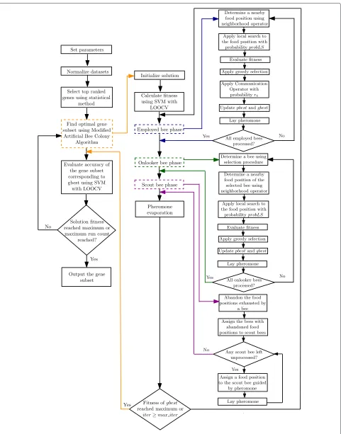
fitness is the output of a single run. It is worth-mentioning that finding a solution with 100 % accuracy is not set as the stopping criteria as further iterations can find a smaller subset with the same accuracy. Ideally, a gene subset con-taining only one gene with 100 % accuracy is the best possible solution found by any algorithm. The proposed modified ABC is given in Algorithm 11 and the flowchart can be found in Fig. 1. The modified ABC algorithm is described next.

Food source positions The position of the food source

for the ith bee Si, is represented by vector Xi =

{x1_X i,x

2 Xi,. . .,x

n

Xi}, wherenis the gene size or dimension of

the data,xd_X

i ∈ {0, 1},i =1, 2,. . .,m(mis the population

size), andd=1, 2,. . .,n. Here,xd_Xi=1 represents that the corresponding gene is selected, whilexd_Xi = 0 means that the corresponding gene is not selected in the gene subset.

to the food source. Accordingly, the indirect communica-tion via pheromone trails enables the ants to find shortest paths between their nest and food sources [169]. The gene subset carrying significant information will occur more frequently. Thus the genes in that subset will get reinforced simultaneously which ensures formation of a potential gene subset. The idea of using pheromone is to keep track of the components that are supposed to be good because they were part of a good solution in pre-vious iterations. Because of keeping this information we need less iterations to achieve a target accuracy. Thus, computational time is also reduced.

Pheromone update The (artificial) pheromone trails are a kind of distributed numeric information [170] which is modified by the ants to reflect their experience accumu-lated while solving a particular problem. The pheromone values are updated using previously generated solutions. The update is focused to concentrate the search in regions of the search space containing high quality solutions. Solution components which are part of better solutions or are used by many ants will receive a higher amount of pheromone, and hence, will be more likely to be used by the ants in future iterations of the algorithm. It indirectly assumes that good solution components construct good solutions. However, to avoid the search getting stuck all pheromone trails are decreased by a factor before getting reinforced again. This mimics the natural phenomenon that, because of evaporation, the pheromone disappears over time unless they are revitalized by more ants. The idea of incorporating pheromone is to keep track of fitness of previous iterations.

The pheromone trails for all the components are rep-resented by the vector P = {p1,p2,· · ·,pn}, where pi

is the pheromone corresponding to the ith gene and n

is the total number of genes. To update the pheromone

picorresponding to the ithgene, two steps are followed:

pheromone deposition, and pheromone evaporation. After each step of update, if the pheromone value becomes greater (less) thantmax(tmin), then the value of pheromone is set to tmax(tmin). Use of tmax, tmin

is introduced in the Max-Min Ant System (MMAS) pre-sented in [61] to avoid stagnation. The value oftminis set to 0 and will be kept same throughout. But the value of

tmaxis updated whenever new global best,gbestsolution is found.

Pheromone deposition After each iteration the bees acquire new information and update their knowl-edge of local and global best locations. The best posi-tion found so far by theithbee is known as thepbesti

and the best position found so far by all the bees, i.e., the population, is known as thegbest. After each bee completes its tasks in each iteration, pheromone

laying is done. The bee deposits pheromone using its knowledge of food locations gained so far. To lay pheromone, theithbee uses its current location (Xi),

the best location found by the bee so far (pbesti), and

the best location found so far by all the bees (gbest). This idea is adopted from Particle Swarm Optimiza-tion (PSO) metaheuristic [171], where the local and global best locations are used to update the velocity of the current particle. We have also used the cur-rent position in pheromone laying to ensure enough exploration though in MMAS [61] only the cur-rent best solution is used to update the pheromone. Only the components which are selected in the corresponding solutions get reinforced. Hence, the pheromone deposition by the ith _{bee utilizes Eq. 4}

below:

pd(t+1)=pd(t)×w+(r0×c0×fi×xdXi)

+(r1×c1×pfi×xd_pbesti) +(r2×c2×gf×xd_gbest)

(4)

Here,d=1, 2,· · ·,n(nis the number of genes),

wis the inertia weight,

fiis the fitness ofXi, pfiis the fitness ofpbesti, gf is the fitness ofgbest,

xd_Xiis selection ofdthgene inXi, xd_pbest

iis selection ofd

th_{gene inpbest} i, xd_gbestis selection ofdthgene ingbest,

c0, c1, andc2determines the contribution of fi, pfi,

andgf respectively,

andr0,r1,r2are random values in the range of [0, 1],

which are sampled from a uniform distribution. Here we have, c0 +c1 + c2 = 1 and c1 = c2.

So the individual best and the global best influence the pheromone deposition equally. The value ofc0

is set from experimental results presented in the Additional file 1.

The inertia weight is considered to ensure that the contribution of global best and individual best is weighed more in later iterations when they con-tain meaningful values. To update the value of inertia weightw, two different approaches have been con-sidered. One approach updates the weight so that an initial large value is decreased nonlinearly to a small value [37].

w(t+1)= (w(t)−0.4)×(MAX_ITER−iter)

MAX_ITER+0.4

(5)

Here, MAX_ITER is the maximum number of

Another approach is to update the value randomly [172].

w= (1+r5)

2 (6)

Here,r5is a random value in the range of [0, 1], which is sampled from a uniform distribution. Per-formance evaluation of each of these two approach is presented in the Additional file 1.

Pheromone evaporation At the end of each iteration, pheromones are evaporated to some extent. The equation for pheromone evaporation is given by Eq. 7:

pi(t+1)=pi(t)×ρ (7)

Here, (1−ρ) is the pheromone evaporation coef-ficient andpiis the pheromone corresponding to the ithgene andnis the total number of genes.pi(t)

rep-resents pheromone value of theithgene after(t−1)th iteration is completed.

Finally, note that, the value oftmaxis updated when-ever a newgbestis found. The rationale for such a change is as follows. Over time, as the fitness ofgbest increases it also contributes more in the pheromone deposition, which may lead the pheromone values for some of the fre-quent genes to reachtmax. At that point, the algorithm will fail to store further knowledge about those particular genes. So we need to update the value oftmaxafter a new

gbestis found. This is done using Eq. 8 below.

tmax(g+1)=tmax(g)×(1+ρ×gf) (8)

Here,tmax(g)represents the value oftmaxwhen thegth

global best is found by the algorithm.

Communication operator We have incorporated a new operator simulating the communication between the ants in a trail. Even though researchers are unable to establish whether such a communication indeed involves informa-tion transfer or not, it is known that foraging decisions of outgoing workers, and their probability to find a recently discovered food source, are influenced by the interactions [62–67]. In fact, there is a large body of evidence empha-sizing the role of ant encounters for the regulation of for-aging activity particularly for harvester ants [62, 68–71]. Even the mere instance of an encounter may provide infor-mation, such as the magnitude of the colony’s foraging activity, and therefore may influence the probability of food collection in ants [72–74].

At each step bees gain knowledge about different components and store their findings by depositing pheromone. After a bee gains new knowledge about the solution components, it share its findings with the succes-sor. So an employed bee gets insight of which components are currently exhibiting excellent performance. Thus a bee

obtains idea about food sources from its predecessor. A gene is selected in the current bee if it is selected in its pre-decessor and pheromone level is greater than a threshold level.

With probabilityr4the followingcommunication

oper-ator (Eqs. 9 and 10) is applied to each employed bee.

The value ofr4is experimentally tuned and the results are

presented in the Additional file 1.

xd_Xi=xd_Xi−1 ×zpd (9)

Where, forithbee

i>1,

d=1, 2,· · ·,n(nis the number of genes), and

zpd=

1, ifpd> tmax₂

0, otherwise (10)

The procedureCommunicate(i)to apply the communi-cation operator onithbee is presented in Algorithm 2.

Algorithm 2:Communicate(i)

1 ford=1 to ndo

2 ifp_d> tmax₂ then 3 zpd =1

4 else 5 zpd =0

6 end 7 xd_X

i=x d

Xi−1×zpd

8 end

Initialization Pheromone for all the genes are ini-tialized to tmax. For all the bees food positions are selected randomly. To initialize the ithbee, the function

initRandom(Si), given in Algorithm 3, is used. Here we

have used a modified sigmoid function that was intro-duced in [37] to increase the probability of the bits in a food position to be zero. The function is given in Eq. 11 below. It allows the components with high pheromone values to get selected.

sigmoid(x)= 1

1+e−x (11)

Here,x≥0 andsigmoid(x)∈[0, 1]

Employed bee phase

Algorithm 3:initRandom(Si)

1 fori=1 to ndo

2 r3=random number in the range of [ 0, 1]

3 ifr3>sigmoid(pj)then

4 xj_X

i=1

5 else 6 xj_X

i=0

7 end 8 end

found neighbor and the current food position. The per-formance and comparison among different local search methods are discussed in the Additional file 1. In each iter-ation the value ofgbest, andpbesti are updated using the

Algorithm 4.

Algorithm 4:UpdateBest(Si)

1 iffitness(S_i) >fitness(pbest_i)then

2 pbest_i=S_i;

3 end

4 iffitness(Si) >fitness(gbest)then

5 gbest=Si;

6 end

Onlooker bee phase

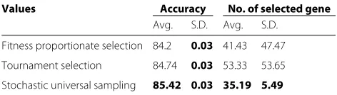
At first a food source is selected according to the good-ness of the source using a selection procedure. As the selection procedure, Tournament Selection (TS), Fitness-Proportionate Selection (FPS), and Stochastic Universal Sampling (SUS) have been applied individually and the results are discussed in the Additional file 1. To deter-mine a new food position the neighborhood operator is applied to the food position of the selected bee. Then local search is applied with the probabilityprobLS to exploit the food position. As local search methods Hill Climbing, Simulated Annealing, and Steepest Ascent Hill Climbing with Replacement are compared. Then greedy selection is applied between the newly found neighbor and the cur-rent food position. In each iteration the value ofgbest, and

pbestiare updated using the Algorithm 4.

Selection procedure In the onlooker bee phase, an employed bee is selected using a selection procedure for further exploitation. As has been mentioned above, tour-nament selection, fitness-proportionate selection, and stochastic universal sampling have been applied individu-ally as the selection procedure.

Tournament selection In this method the fittest individ-ual is selected among thetindividuals picked from the population randomly with replacement [173],

where t ≥ 1. Value of t is set to 7 in our

algo-rithm. This selection procedure is simple to imple-ment and easy to understand. The selection pressure of the method directly varies with the tournament size. With the increase of the number of competi-tors, the selection pressure increases. So selection pressure can easily be adjusted by changing the tour-nament size. If the tourtour-nament size is larger, weak individuals have a smaller chance to be selected. The pseudocode is given in Algorithm 5.

Algorithm 5:TorunamentSelection()

1 Best=individual picked at random

2 fori from 2 to tdo

3 Next=individual picked at random

4 iffitness(Next) >fitness(Best)then

5 Best=Next 6 end

7 end 8 returnBest

Fitness-proportionate selection In this approach, indi-viduals are selected in proportion to their fitness [173]. Thus, if an individual has a higher fitness, its probability of getting selected is higher. In fitness-proportionate selection which is also known as roulette wheel selection, even the fittest individual may never be selected. In basic ABC, roulette wheel or fitness-proportionate selection scheme is incor-porated. The analogy to a roulette wheel can be envisaged by imagining a roulette wheel in which each candidate solution represents a pocket on the wheel; the size of the pockets are proportionate to the probability of selection of the solution. Select-ingN individuals from the population is equivalent to playingN games on the roulette wheel, as each candidate is drawn independently. The pseudocode is given in Algorithm 6.

Algorithm 6:FitnessProportionateSelection()

1 f1=fitness(S1)

2 fori from 2 to Ndo

3 fi=fitness(Si)

4 fi=fi+fi−1

5 end

6 r=random number in the range [ 0,f_N]

7 fori from 2 to tdo

8 iffi−1<r≤fithen

9 returnSi

10 end 11 end 12 returnS₁

methods. In SUS, selection is done in a fitness-proportionate way but biased so that fit individuals always get picked at least once. This is known as

a low variance resampling algorithm. SUS is used

in genetic algorithms for selecting potentially use-ful solutions for recombination. The method has become now popular in other venues along with evolutionary computation [173]. The pseudocode is given in Algorithm 7.

Algorithm 7:StochasticUniversalSampling(Ns)

1 f1=fitness(S1)

2 index=0

3 fori from 2 to Ndo

4 fi=fitness(Si)

5 f_i=f_i+f_i−1 6 end

7 r=random number in the range [0,_NfN

s]

8 fori from 2 to N_sdo

9 whilef_index<rdo

10 index=index+1

11 end

12 r=r+fN/Ns

13 ini=index

14 end

15 q=random number in the range [0,N_s] 16 returnSinq

Other methods like roulette wheel can have bad performance when a member of the population has a really large fitness in comparison with other mem-bers. SUS starts from a small random number, and chooses the next candidates from the rest of popula-tion remaining, not allowing the fittest members to saturate the candidate space.

Scout bee

If the fitness of a bee remains the same for a prede-fined number (limit) of iterations, then it abandons its food position and becomes a scout bee. In basic ABC, it is assumed that only one source can be exhausted in each cycle, and only one employed bee can become a scout. In our modified approach we have removed this restriction. The scout bees are assigned to new food positions randomly. While determining components to form a new food position the solution component with higher pheromone values have higher probability of being selected. The value of limit is experimentally tuned and discussed in the Additional file 1. The variable

triali contains the number of times the fitness remains

unchanged consecutively for the ith _{bee. The procedure}

initRandom(Si) to assign new food positions for scout

bees is given in Algorithm 3. In each iteration the value of

gbest, andpbestiare updated using the Algorithm 4.

Local search

To explore nearby food sources the basic ABC algo-rithm applies a neighboring operator to the current food source. But in our algorithm we have applied local search to produce a new food position form the current one. In the employed bee and onlooker bee stages, local search is applied with the

probabil-ity probLS to increase the exploitation ability [95]. The

value of probLS is scientifically tuned in the Additional file 1. As has already been mentioned above, as the local search procedures, Hill Climbing (HC), Simu-lated Annealing (SA), and Steepest Ascent Hill Climb-ing with Replacement (SAHCR) have been employed as the local search procedure. Depending upon the choice HillClimbing(S) or SimulatedAnnealing(S) or

SteepestAscentHillClimbingWithReplacement(S)is called

form the method LocalSearch(S). The performance

assessment between different local searches and the parameter tuning of the local search methods are dis-cussed in the Additional file 1.

Algorithm 8:HillClimbing(S)

1 repeat

2 R=Tweak(S)

3 iffitness(R) >fitness(S)then

4 S=R 5 end

6 untilthe stopping criteria are met; 7 returnS

Simulated annealing Annealing is a process in metal-lurgy where molten metals are slowly cooled to make them reach a state of low energy where they are very strong. Simulated annealing is an analogous optimization method for locating a good approxima-tion to the global optima. It is typically described in terms of thermodynamics. Simulated annealing is a process where the temperature is reduced slowly, starting from mostly exploring by random walk at high temperature eventually the algorithm does only plain hill climbing as it approaches zero temperature. The random movement corresponds to high tem-perature. Simulated annealing injects randomness to jump out of the local optima. At each iteration the algorithm selects the new candidate solution proba-bilistically. So the algorithm may sometimes go down hills. The pseudocode is given in Algorithm 9.

Algorithm 9:SimulatedAnnealing(S)

1 initilaizet 2 best=S 3 repeat

4 R=Tweak(S)

5 r= a random number in the range of [ 0, 1]

6 iffitness(R)>fitness(S)or r<e

fitness(R)−fitness(S)

t _then

7 S=R 8 end

9 t=t−2×schedule

10 iffitness(S)>fitness(best)then

11 best=S 12 end

13 untilthe stopping criteria are met; 14 returnS

Steepest ascent hill climbing with replacement This method samples all around the original candidate solution by tweakingn times. Best outcome of the tweaks is considered as the new candidate solution. The current candidate solution is replaced by the new one rather than selecting the best one between

the new candidate solution and the current solu-tion. The best found solution is saved in a separate variable. The pseudocode is given in Algorithm 10.

Algorithm 10:SteepestAscentHillClimbingWithReplace−

ment(S)

1 best=S 2 repeat

3 R=Tweak(S)

4 fornt−1timesdo

5 W =Tweak(S)

6 iffitness(W)>fitness(R)then

7 R=W 8 end 9 end 10 S=R

11 iffitness(S)>fitness(best)then

12 best=S 13 end

14 untilthe stopping criteria are met; 15 returnS

Neighborhood operator In the solution we need only the informative genes to be selected. So we discard the uninformative ones from the solution. By this way we will get a small set of informative genes. To find a nearby food position we first find the genes which are selected in the current position. A number of selected genes (at least one) are dropped from the current solution. We get rid of the genes which tend to appear less potential. If the current solution has zero selected genes then we rather select a possibly informative gene. The parame-ternddetermines the percentage of selected genes to be removed. The value ofndis experimentally tuned in the Additional file 1.

LetXe= {0, 1, 1, 0, 1, 0, 0, 1, 1, 0, 1, 1, 1, 0, 0, 1, 0, 1, 0, 0}is

a candidate solution with gene size,n=20 and the num-ber of selected gene is 10 (ten). So ifnd = 0.3 we will randomly pick 3 (three) genes which are currently selected in the current candidate solution(Xe) and change them

to 0. Let the indices 2 (two), 8 (eight), and 15 (fifteen) are randomly selected. Sox2_Xe,x8_Xe, andx15_Xewill become zero. Nearby food position(Xn

e)of the current candidate

solu-tion(Xe), found after applying the neighborhood operator

will beXn

e = {0, 1,0, 0, 1, 0, 0, 1,0, 0, 1, 1, 1, 0, 0,0, 0, 1, 0, 0}

(changes are shown inboldfacefont). Please note that we adopt zero-based indexing.

selected, after tweak it will be dropped and vice versa. For example letXe = {0, 1, 1, 0, 1, 0, 0, 1, 1, 0, 1, 1, 1, 0, 0, 1, 0, 1,

0, 0} is a candidate solution with gene size, n = 20

and the number of selected gene is 10 (ten). Let ran-domly the index 6 (six) is selected. So the tweaked food position (Xt_e) of the current candidate solution (Xe), found after applying the tweak operator will

be X_et = {0, 1, 1, 0, 1, 0,1, 1, 1, 0, 1, 1, 1, 0, 0, 1, 0, 1, 0, 0} (change is shown inboldfacefont). Please note that we adopt zero-based indexing.

Fitness Our fitness function has been designed to con-sider both the classification accuracy and the number of selected genes. The higher the accuracy of an individual the higher is its fitness. On the other hand small number of selected genes yields good solution. So if the percent-age of genes that are not selected is higher the fitness will be higher. The value n−nsi

n gives the percentage of genes

that are not selected in Si. The tradeoff between weight

of accuracy and selected gene size is given byw1. Higher value ofw1means accuracy is prioritized more than the selected gene size. So, finally the fitness of theithbee(Si)

is determined according to Eq. 12.

fitness(Si)=w1×accuracy(Xi)+(1−w1)×

n−nsi

n

(12)

Here, w1 sets the tradeoff between the importance of

accuracy and selected gene size,Xi is the food position

corresponding toSi,accuracy(Xi)is the LOOCV (Leave

One Out Cross Validation) classification accuracy using SVM (to be discussed shortly), andnsi is the number of

currently selected genes inSi.

Accuracy To assess the fitness of a food position we need the classification accuracy of the gene subset. The predic-tive accuracy of a gene subset obtained from the modified ABC is calculated by an SVM with LOOCV (Leave One Out Cross Validation). The higher the LOOCV classifi-cation accuracy, the better the gene subset. SVM is very robust with sparse and noisy data. SVM has been found suitable for classifying high dimensional and small-sample sized data [142, 175]. Also SVM is reported to perform well for gene selection for cancer classification [20, 176].

The noteworthy implementations of SVM include SVMlight[177], LIBSVM [178], mySVM [179], and BSVM [180, 181]. We have included LIBSVM as the implemen-tation of SVM. For a multi-class SVM, we have utilized the OVO (“one versus one") approach, which is adapted in the LIBSVM [178]. The replacement of dot product by a nonlinear kernel function [182] yields a nonlinear mapping into a higher dimensional feature space [183]. A kernel can be viewed as a similarity function. It takes two inputs and outputs how similar they are. There are

four basic kernels for SVM: linear, polynomial, radial basic function (RBF), and sigmoid [184]. The effective-ness of SVM depends on the selection of kernel, the kernel’s parameters, and the soft margin parameter C. Uninformed choices may result in extreme reduction of performance [142]. Tuning SVM is more of an art than an exact science. Selection of a specific kernel and relevant parameters can be achieved empirically. For the SVM, the penalty factorCandGammaare set to 2000, 0.0001, respectively as adopted in Li et al. [41]. Use of linear and RBF kernel and their parameter tuning is discussed in the Additional file 1.

As classifier for both binary class and multi class gene selection methods, use of SVM is present in [23, 37, 41, 42, 45, 54, 153, 157, 164, 165, 185–200].

Cross-validation is believed to be a good method for selecting a subset of features [201]. LOOCV is in one extremity ofk-fold cross validation, wherekis chosen as the total number of examples. For a dataset withN exam-ples,Nnumbers of experiments are performed. For each experiment the classifier learns onN −1 examples and is tested on the remaining one example. In the LOOCV method, a single observation from the original sample is selected as the validation data, and the remaining obser-vations serve as training data. This process is repeated so that each observation in the sample is used once as the validation data. So every example is left out once and a prediction is made for that example. The average error is computed by finding number of misclassification and used to evaluate the model. The beauty of the LOOCV is that despite of the number of generations it will generate the same result each time, thus repetition is not needed.

Pseudocode for the modified ABC algorithm Finally, the pseudocode of our modified ABC algorithm used in this article is given in Algorithm 11 and the flowchart of the proposed gene selection method using Algorithm 11 is given in Fig. 1.

Results and discussion

Algorithm 11:modified Artificial Bee Colony Algorithm

// initialization

1 fori=1 to ndo

2 pi=tmax;

3 end

4 fori=1 to Ndo

5 initRandom(S_i);

6 end 7 PS=N; 8 repeat

// Employed Bee Phase

9 fori=1to PSdo

// produce a new solution using the neighborhood operator

10 E=Neighbor(S_i);

// apply local search with probability probLS

11 E=LocalSearch(E);

12 iffitness(E) >fitness(S_i)then

13 Si=E;

14 end

15 Communicate();

16 UpdateBest(S_i);

17 LayPheromone;

18 end

// Onlooker Bee Phase

19 fori=1to PSdo

// select a bee index using the selection procedure

20 j=Selection();

// produce a new solution using the neighborhood operator form the selected bee

21 O=Neighbor(S_i);

// with probability probLS apply local search

22 O=LocalSearch(O);

23 iffitness(O) >fitness(Si)then

24 Si=O;

25 end

26 UpdateBest(Si);

27 LayPheromone;

28 end

// Scout Bee Phase

29 fori=1to PSdo

30 iftriali>limitthen

31 initRandom(Si);

32 UpdateBest(Si);

33 LayPheromone;

34 end 35 end

36 Evaporate Pheromone;

37 untilthe stopping criteria are met;

38 Gene subset corresponding togbestis the optimal

subset found by the algorithm

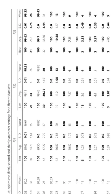
of different parameters are discussed in the Additional file 1. Comparison with previous methods that used the same datasets is discussed in this section. We have also presented comparison between different known heuristics methods in this section. Four different parameter settings according to different criteria have been proposed in this paper. Performance comparison for all the parameter set-tings is given in this section. In all cases the optimal results (maximum accuracy and minimum selected gene size) are highlighted usingboldfacefont.

Datasets

Brief attribute summary of the datasets are presented in Table 1. The datasets contains both binary and multi class high dimensional data. The online supplement to the datasets [192] used in this paper is available at http://www. gems-system.org. The datasets are distributed as Matlab data files (.mat). Each file contains a matrix, the columns consist of diagnosis (1st column) and genes, and the rows are the samples.

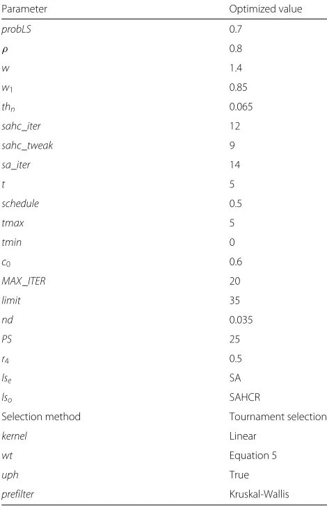
Optimized parameter values

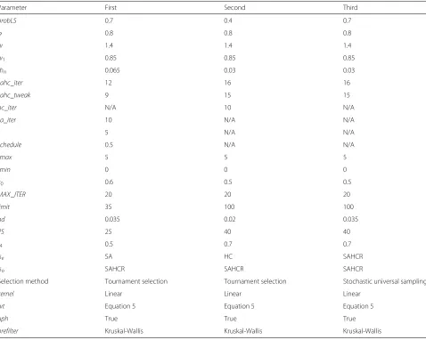
While selecting the optimized parameter setting (Table 5) we have considered other factors besides the obtained performance.

After analyzing the results (Table S3 in Additional file 1), we have decided to use 0.5 as the value ofr4in our final experiments. Probability value of 0.7 for local search has been used to ensure that too much exploitation is not done despite that the value of 1.0 gives the highest accu-racy (Table S5 in Additional file 1). The value ofndis set to 0.035 as it demonstrates a good enough accuracy with tolerable gene set size among all the values considered for the parameter (Table S6 in Additional file 1). Popula-tion size is kept at 25 which shows an acceptable level of accuracy (Table S9 in Additional file 1). We have selected SAHCR as the local search method at the onlooker bee stage and SA at the employed bee stage to ensure both exploration and exploitation. The value 12 is set as iter-ation count of SAHCR as it shows acceptable accuracy (Table S19 in Additional file 1). The value is kept small because increased iteration count increases the algorithm running time. The value 9 is considered as the final value for number of tweaks in SAHCR (Table S20 in Additional file 1). The value 0.065 is selected as the percentage of genes to be preselected in the preprocessing stage despite that the value 0.03 gives the best accuracy (Table S21 in Additional file 1). This is done because choosing 0.03 might possess the risk of discarding informative genes in the prefiltering step for other datasets. The value 0.6 is set forc0 as it shows good results (Table S23 in Additional

file 1). The obtained accuracy is highest for thelimitvalue 100 (Table S25 in Additional file 1). But high value oflimit