Derivative Application in Navigation into Outerspace

D

D

E

E

R

R

I

I

V

V

A

A

T

T

I

I

V

V

E

E

A

A

P

P

P

P

L

L

I

I

C

C

A

A

T

T

I

I

O

O

N

N

I

I

N

N

N

N

A

A

V

V

I

I

G

G

A

A

T

T

I

I

O

O

N

N

I

I

N

N

T

T

O

O

O

O

U

U

T

T

E

E

R

R

S

S

P

P

A

A

C

C

E

E

M

M

i

i

h

h

a

a

i

i

Ș

Ș

.

.

N

N

e

e

a

a

m

m

ț

ț

u

u

,

,

M

M

i

i

h

h

a

a

e

e

l

l

a

a

N

N

e

e

a

a

m

m

ț

ț

u

u

1

National College Constantin Diaconovici Loga Timișoara - Romania, Department of Mathematics

2 _{West University of Timișoara - Romania, Department of Economics and Modelling}

Corresponding Author: Mihaela Neamțu, [email protected] ABSTRACT: The aim of the present paper is to use the

first order mathematical derivative to explain the return trajectory of an object, in our particular case it is about a spaceship belonging to NASA Apollo 13 Space Program. Firstly, the mission overview is presented followed by the mathematical modelling pertaining to this case study. We focus on the events that could follow an unforeseen accident. More precisely, we take into consideration three types of the return trajectory that the spaceship could have followed: a ricochet in outer space, crashing on the Earth’s surface and safe landing on Earth. The numerical simulations are done using GeoGebra software. Finally, conclusions are drawn.

KEYWORDS: first order derivative, mathematical modelling, applications, object trajectory, numerical simulations.

1. INTRODUCTION

Mathematical modelling is an important tool used to describe, analyze and predict complex natural phenomenon and processes. Therefore, the evironment can be simplified, emulated and understood in an efficient way. Based on ([MG14]), [MSC07]), many countries apply the approach of modelling in teaching and learning processes. In the teaching process it is important to help pupils to discover and apply knowledge flexibly for studying more effectively ([Tinh17]). Nowdays, the trends in education highlight the strong connection between mathematical knowledge and the real world applications ([CQ17]).

In the present paper, we use the mathematical derivative of the first order to model, explain and describe the return trajectory of a spaceship.

In an attempt to set foot on the Moon again, NASA embarked on a new space mission named Apollo 13. An unfortunate accident took place on the way to the Moon that changed completely the entire flight plan and scope of the mission. During the attempt to stir the oxygen tanks an explosion occurred that put in danger the human crew of Apollo 13. Following this accident there were three types of the return trajectory that the spaceship could follow: a ricochet in outer space, crashing on the Earth’s surface and safe landing on Earth. These orbits of the spaceshift

can be interpretated using the mathematical modelling.

The structure of the paper is as follows. Section 2 describes Apollo 13 mission overview. Throughtout Section 3 the mathematical modelling pertaining to the case study is addressed. GeoGebra software is used to illustrate numerical simulations. Finally, conclusions are drawn and presented in Section 4.

2. APOLLO 13 MISSION

Apollo 13 was the seventh mission in the Apollo space program and the third intended to land on the Moon. The craft was launched on April 11, 1970, at 14:13 EST (19:13 UTC) from the Kennedy Space Center, Florida, but the lunar landing was aborted after an oxygen tank exploded two days later. A lot of problems were caused by limited power, like loss of cabin heat, shortage of potable water, and the critical need to repair the carbon dioxide removal system. After the explosion, they were faced with two dangerous options for the return trajectory to Earth: one being to turn around immediately and the other one was to continue they journey toward the Moon using its gravity to put them on return trajectory to Earth. They took the decision not to turn around immediately, but to use the Moon gravity. They shut down all the electrical power consuming systems (including the guiding system) with the exception of the communication system.

On their journey back in one point in time they had to manually orient the spaceship on the right trajectory that gave them the optimal gravitational force for a safe landing on Earth.There are three possibilities:

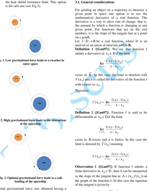
1. Low gravitational force will result into a ricochet in outer space. The spaceship and its crew will be lost in space (see Fig. 1). 2. High gravitational force will result into a

3. Optimal gravitational force will result into a descending speed that generates heat below the heat shield resistance limit. This option is the safe one (see Fig 3).

Fig. 1. Low gravitational force leads to a ricochet in outer space

Fig. 2. High gravitational force leads to the distruction of the spaceship

Fig. 3. Optimal gravitational force leads to a safe landing of the spaceship

Optimal gravitational force was obtained having a flight path defined by the right Earth orbit tangent. In mathematical terms the equation of the tangent is

3. MATHEMATICAL APPROACH

3.1. General considerations

For guiding an object on a trajectory to intersect a given point in space one option is to use the mathematical derivative of a real function. The derivative is a way to show rate of change: that is, the amount by which a function is changing at one given point. For functions that act on the real numbers, it is the slope of the tangent line at a point on a graph.

Let f:DRbe a real function, where D is an interval or an union of intervals within R.

Definition 1 ([Gan97]). We say that function f admits a derivative in x₀Dif the limit

0 0 x

x _{x x}

) x ( f ) x ( f lim o   

exists in R. In this case the limit is denoted with

) x (

f 0 and it is called the derivative of the function f with respect to x₀.

Therefore, . x x ) x ( f ) x ( f lim ) x ( f 0 0 x x 0 o     

Definition 2 ([Gan97]). Function f is said to be differentiable at x₀Dif the limit

0 0 x

x _{x x}

) x ( f ) x ( f lim o   

exists in R(exists and it is finite). In this case the limit is denoted by f(x₀)meaning

. x x ) x ( f ) x ( f lim ) x ( f 0 0 x x 0 o     

Observation 1 ([Gan97]) If function f admits a finite derivative in x₀D, then it can be interpreted as the slope of the tangent line at A(x₀,f(x₀))on the graph of the function f. In this case the equation of the tangent is given by:

). x x )( x ( f ) x ( f

3.2. Numerical examples

We suppose the equation of the Earth's atmospheric shape is given by the function

f:[-5,5]->R,

3 x 7 ) x ( f

2



 .

Based on the above function, in what follows, using GeoGebra we want to visualize three cases of the spaceship’s trajectory, where the gravitational force is low, high and optimal, respectively.

Let us have the spaceship’s position defined by S having the coordinates as(5,5).

In the first the case we do not have a safe landing due to a low gravitational force that will result into a ricochet in outer space of the spaceship. The trajectory of the spaceship will intersect the point with the coordinates A=(-4,2) and the equation is given by:

x-3y+10=0.

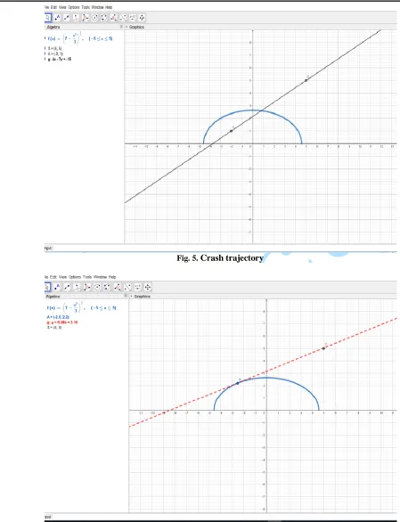
In the second case, we do not have a safe landing due to high gravitational force that will result into a descending speed that generates heat above the heat shield resistance limit.

The trajectory of the spaceship will intersect the point with the coordinates A=(-2, 1) and the equation is given by:

4x-7y+15=0.

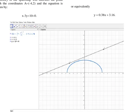
In the third case, in order to assure a safe landing the option is to follow a trajectory which is tangent to Earth’s atmosphere. If we choose to reach the point with the coordinates A=(-2.5, 2.2), the equation of the tangent of f at the point A is given by:

) 5 . 2 x )( 5 . 2 ( f ) 5 . 2 ( f

y     

or equivalently

. 16 . 3 x 38 . 0

y 

Fig. 5. Crash trajectory

Fig. 6. Optimal trajectory

CONCLUSIONS

Nowdays, in the educational process it is of paramount importance the link between the theoretical concepts

function with a single real variable.

REFERENCES

[CQ17] T.V. Cuong, L. H. Quang – Teaching mathematical modeling: connecting to

classroom and practice, Annals.

Computer Science Series, 15(2), 2017. [Gan97] M. Ganga – Basics of mathematical

analysis, MathPress House Publishing,

1997.

[MG14] S. Mehraein, A. R. Gatabi – Gender

and mathematical modelling

competency: primary students’

performance and their attitude, Social and Behavioral Sciences 128, 2014.

[MSC07] N. Mousoulides, B. Sriraman, C. Christou – From problem solving to modeling. The emergence of models

and modleling perspectives, Nordic

Studies in Mathematics Education, 12(1), 2007.

[Tin17] T. T. Tinh – Development

thechers’mathematics competency

through teaching complex numbers in

high school in Vietnam, Annals.

Computer Science Series, 15(2), 2017. [***]

https://airandspace.si.edu/explore-and-