On the Matrices of Pairwise Frequencies of Categorical Attributes for Objects Classification

(1)

https://www.scirp.org/journal/jilsa ISSN Online: 2150-8410 ISSN Print: 2150-8402

DOI: 10.4236/jilsa.2019.114004 Sep. 30, 2019 65 Journal of Intelligent Learning Systems and Applications

On the Matrices of Pairwise Frequencies of

Categorical Attributes for Objects Classification

Vladimir N. Shats

St. Petersburg, Russia

Abstract

This paper proposes two new algorithms for classifying objects with categori-cal attributes. These algorithms are derived from the assumption that the attributes of different object classes have different probability distributions. One algorithm classifies objects based on the distribution of the attribute fre-quencies, and the other classifies objects based on the distribution of the pair-wise attribute frequencies described using a matrix of pairpair-wise frequencies. Both algorithms are based on the method of invariants, which offers the sim-plest dependencies for estimating the probabilities of objects in each class by an average frequency of their attributes. The estimated object class corres-ponds to the maximum probability. This method reflects the sensory process models of animals and is aimed at recognizing an object class by searching for a prototype in information accumulated in the brain. Because these matrices may be sparse, the solution cannot be determined for some objects. For these objects, an analog of the k-nearest neighbors method is provided in which for each attribute value, the class to which the majority of the k-nearest objects in the training sample belong is determined, and the most likely class value is calculated. The efficiencies of these two algorithms were confirmed on five databases.

Keywords

Categorical Attributes, Classification Algorithms, Invariants of Matrix Data, Data Processing

1. Introduction

The solution to the classification problem is reduced to calculating a function that divides a training sample (TRS) into classes and simultaneously obtains an acceptable classification accuracy for a test sample (TS). In most existing

me-How to cite this paper: Shats, V.N. (2019) On the Matrices of Pairwise Frequencies of Categorical Attributes for Objects Classifi-cation. Journal of Intelligent Learning Sys-tems and Applications, 11, 65-75.

https://doi.org/10.4236/jilsa.2019.114004

Received: May 28, 2019 Accepted: September 27, 2019 Published: September 30, 2019 Copyright © 2019 by author(s) and Scientific Research Publishing Inc. This work is licensed under the Creative Commons Attribution International License (CC BY 4.0).

(2)

DOI: 10.4236/jilsa.2019.114004 66 Journal of Intelligent Learning Systems and Applications

thods, algorithms for calculating these functions have considerable computa-tional complexity [1] [2] [3]. In previous work [4], the method of invariants (MI) was proposed, where this function is a linear combination of the simplest functions of the values of each feature that qualitatively simplifies the computa-tion algorithm. It was shown in [5] that the MI corresponds to sensory process models of animals, which aim to recognize an object’s class by searching for a prototype in the information accumulated in the brain.

The MI proceeds from the fact that in classification problems, the accuracy of the data plays a special role since the objects, their descriptions, and their classes are correlated, and each type of entity has a randomness component. Therefore, a given data matrix is just one of possible random realization of the matrices that form the set of invariants with respect to the class. This approach is consistent with the concept proposed by L. Zadeh, which says that for most manually solved tasks, high accuracy is not required because the brain perceives only a “trickle of information” about the external world [6]. Moreover, for systems whose complexity exceeds a certain threshold, accuracy and practical sense are almost mutually exclusive characteristics.

In the MI, the range of attribute values after randomization, accompanied by an introduction of an additive component that follows a uniform distribution, is divided along each attribute into equal numbers of intervals, within which the feature values are assumed to be equiprobable. All objects falling within the in-terval receive an index of the corresponding attribute equal to the inin-terval num-ber.

For each index, one can find lists of numbers of TRS objects of a certain class and then calculate the frequencies of the indices. With some error, these fre-quencies will be the same for the objects in the TRS and the TS because both samples belong to the same general population. Therefore, it is possible to esti-mate the probability of the individual attributes of any object in each class. Then, using the simplest formula of the total probability, estimate the probability of an object having a specific set of feature values. Finally, the class of the object is de-termined based on the maximum likelihood principle.

There is an obvious analogy between indices and categories, the values of which can always be described by a finite sequence of integers 1, 2... Therefore, the MI serves as the basis for this article, in which two algorithms are proposed: one implements the simplest version of the MI developed for quantitative attributes, and the other more fully takes the features of categorical attributes into account.

The efficiency of the new algorithms was tested on five databases [7].

2. Assumptions and Preliminary Assumptions

The article is devoted to solving classification problems for which all attributes are categorical. The solution is based on two MI assumptions:

(3)

For categorical attributes, the number of values or levels n that individual ob-jects can take is an important characteristic of the problem. In real tasks for quantitative attributes, the value of nq, as a rule, considerably exceeds that of

c

n —the corresponding value for categorical attributes. According to the theory proposed by C. Shannon, the information volume per value of a feature increas-es in proportion to the value of log2

( )

nq log2

( )

nc . Therefore, in tasks involv-ing categorical features, the “information load” of the data often increases sever-al fold. This circumstance manifests in an increase in the number of objects of different classes that have the same attribute values. This reduces the difference between the attribute frequencies for objects of different classes, which can lead to an increase in the number of classification errors.

However, categorical attributes also have “favorable” features. The probability of an object of a certain class is an unknown function of its attributes, which takes into account the interrelations among all the attributes. Usually, this func-tion is nonlinearly dependent on the attribute values of the object. This rela-tionship is indirectly taken into account in the accepted assumption of the MI, since the frequencies of attribute indices are calculated for a particular class of objects. Then, this dependence becomes linear, which greatly simplifies algo-rithm’s calculation. One algorithm takes the same approach for categorical attributes whose values are, as noted above, analog indices.

The second algorithm considers the peculiarities of categorical attributes in a different way and is based on a new solution to the question of attribute rela-tionships. Usually, the relationship between random variables is estimated using the Pearson correlation coefficient or the rank correlation coefficient. However, in the framework for this method, we are interested in the frequencies of attribute values that take a relatively small number of values. The paper further shows that pairwise frequencies of features allow an approximate assessment of the relationship between the features of objects of the same class (note that, as a rule, only a weak correlation exists between the categorical features of objects in the same class).

However, pairwise frequencies do not allow the determination of the class of TS objects if no object has the same combination of attribute values in the TRS. To classify objects, this algorithm uses an analog of the k-nearest neighbors me-thod: the object is assigned to a class for which the total number of the k-nearest neighbors of the TRS’ objects for each attribute are maximized.

3. Two Algorithms for Solving the Classification Problem

3.1. Statement and Basic Algorithm

Let the vectors Xk,k∈

(

1,N

)

describe the values of categorical attributes

ob-jects, which form the TRS

{

(

X_s,y_s

)

|s∈

(

1,M

)

}

, where y is the vector of the

ob-ject class labels, M is the number of objects, and missing data are excluded. With-out loss of generality, we assume that the values of the attributes Xk,k∈

(

1,N

)

and classes (possibly after preliminary encoding) belong to the sets of integers

(

1, k

)

(4)

of attribute Xk and С is the number of classes. The problem is to classify the

TS objects.

We denote s objects by

(

)

T 1, , s = xs xsN

x  and the data matrix by

sk M N

x _×

=

Q . Consider the algorithm for the basic MI (algorithm 1). Using

ma-trix Q, we find lists ω_i =

{

s s| ∈

(

1,M

)

,y_s =i

}

of numbers of objects of class

{ }

1,

i∈ C . The sample probability of objects in class i determines the obvious dependence:

( )

{

1 1, , | ,

(

1,

)

}

i s N sN i

p x = p X =x  X =x s∈ω k∈ N . (1)

This dependence allows finding objects whose attribute value xk = j. Let 0

kj

r ≥ denote the number of such objects. Then, the frequency of a value j for an attribute k of the TRS object of class i equals

( )

fkj _i =rkj li , where li = ωi .

Object x arises as a result of appearances of each attribute k with the

cor-responding value j. Since these events form a complete group of incompatible events, the total probability formula gives an estimate of the probability that an object belongs to class i:

( )

1

( )

1 M

i k kj _i

p f

N =

=

∑

x , (2)

where j is the value of attribute k for object x.

Formulas (1) and (2) yield a class probability estimate for the TRS objects. Since TRS and TS belong to a single general population, the formula also deter-mines the frequencies of the TS objects. According to the maximum likelihood principle, the calculated class of the object x is

( )

arg maxi( )1,C i

( )

.

I x = _∈ p x (3)

3.2. Features of the Model of Probability Density Objects

Essentially, the MI is based on the assumption that a class of objects can be rec-ognized by the probability distribution of its attributes. According to (2), the probability p xi

( )

received its point estimate equal to the average frequencies

attributes of object x of class i. Thus, the empirical frequency distribution of

features is transformed into the frequency distribution of objects. Therefore, the MI considers the average composition of the attribute distribution as a probabil-ity distribution for objects of a particular class.

We investigate the characteristics of this distribution in the case of two attributes that have typical forms of attribute frequency distributions. Our analysis showed that the distributions of each attribute can be considered a sample of the theo-retical distributions described by unimodal laws, the maximum of which is lo-cated in the middle and the “tails” of the distribution.

Consider the following task. Let objects have two categorical attributes, the values of which describe random variables Y and Z with probability densities

( )

2 2

y

b y

a y

ϕ =

+ and

( )

2 z z c d z g z

(5)

( )

0,

z∈ n , and a b c d g h, , , , , and n are parameters. From formula (2), a random

variable U =

(

Y+Z

)

2 is the composition of Y and Z, which simulates the total

distribution of the objects. We are interested in the features of this distribution. Note that the functions ϕy

( )

y and ϕz

( )

z allow us to obtain an analytical

solution for the distribution composition of the above types of attributes. Since these functions determine the corresponding density distribution, their parame-ters are related by the following:

( )

0 d 1

n

Y y y

ϕ =

∫

,

∫

₀nϕ_Z

( )

z dz=1.

Obviously, U= +Y Z, where Y=Y 2 and Z=Z 2 are random variables

[8]. Given that density ϕy

( )

y =ϕ µy

(

( )

y

)

µ′

( )

y , µ

( )

y =2y , we obtain

( )

2 2

2 4 y b y a y ϕ = +  

 . Similarly, we find that

( )

(

)

2

2 2 4

z z c d z g z

ϕ_  = ∗ + ∗ ∗ + ∗ ∗  .

The density ϕU

( )

u is a convolution of the functions

ϕ

Y and ϕz

( )

z :

( )

₀

( ) (

)

d

U Z

u Y

u y u y y

ϕ =

_∫

ϕ_  ϕ_ − .

The range of u is divided into segments: 0≤ ≤u n 2 and n 2< ≤u n. Be-cause z≥0, the lower and upper limits of the integrals are equal to 0 and u for

the first segment and u−n 2 and u for the second segment, respectively. Then,

we can obtain the formula for calculating the density:

( )

3

( )

1

4

U u b q A w uq q

ϕ = ∗

∑

₌ ,

where 2

1 2 4

A = + ∗ ∗ + ∗ ∗c d u g u , A2 = − ∗ + ∗ ∗

(

2 d 8 g u

)

, A3= ∗4 g

( )

1 2 2 0 1 2 2 2

d 0 2

4 d 2 4 q u q _q u u n y

y u n

a y

w u

y

y n u n

a y − − −  ≤ ≤  _{+ ∗}  = 

 _{< ≤}

 _{+ ∗} 

∫

 _   _ 

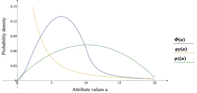
Sub-integral functions are tabulated and not given for the abbreviated entries. We performed calculations were performed for a wide range of parameters. The results are illustrated in Figure 1, where the density ϕu is determined for

the case in which the density ϕz follows a normal distribution, and the

ϕ

y

distribution is close to hyperbolic. The figure shows that with respect to the curve ϕz, the ordinates of curve ϕu increase in the region of high values of

density

ϕ

y and decrease in sections with low values. Consequently, the

func-tion ϕu does not follow a normal distribution. However, confidence intervals

of continuous random variables can be estimated only for normal distributions. From the analysis, it should be noted that the composition distributions of in-dividual attributes result in a poorly predictable distribution for certain classes of objects. Thus, the effectiveness of the various MI algorithms depends on the data characteristics for a particular task and can be tested only empirically.

3.3. Algorithm 2

(6)

[image:6.595.211.538.74.229.2]

Figure 1. Density curves of random variables Y, Z and U (ϕ ϕy, z and Φ correspond

to ϕ ϕ_y, _z and ϕu).

from different distributions of features to classify objects according to the fre-quencies of the categorical attribute values. However, another variant of the ap-proximate realization of this assumption is also possible.

For any type of attribute, the probability of an arbitrary object

(

)

T 1, , N

x x

=

x 

of class i is determined by the following relation:

( )

1

( ) (

1 2 2| 1

) (

3 3| 1, 2

)

N

(

N | 1, , N 1

)

P x = p x p x x p x x x p x x  x − , (4)

where pk

(

xk|x1,,xk−1

)

is the conditional probability of an attribute Xk at

values x1,,xk−1 of attributes X1,,Xk−1. Here, p x1

( )

1 is found by formula

(1).

Consider the features of this dependence for categorical attributes. Here, the elements of the set of Cartesian products of the attributes Xk and Xk+1,

(

1, 1

)

k∈ N− are ordered pairs:

(

x x k, k+1

)

, where xk∈

{ }

1,nk and

{

}

1 1, 1

k k

x₊ ∈ n ₊ . Let i_, ₁ k k

e ₊ be the number of objects of class iwhose attributes

correspond to a pair

(

x x k, k+1

)

. Then, the frequency of the pair , 1 , 1

i i

k k k k i

f ₊ =e ₊ l

gives the sample estimate probability of the pair for object x of class i. The set

of frequencies defines a matrix

1 , 1

k k

i i

k k gw _n _n

R f

+

+ = _× ,

constructing a matrix of pairwise frequencies (MPF) for the attributes k and

1

k+ for the TRS objects of class i. There are N−1 MPFs for each class.

Ac-cording to the concept formed by the above matrix, we can define the properties of the TRS and TS objects. Then, from formula (4), we obtain the approximate dependence for estimating the probability that object x belongs to class i

( )

1

( )

1 1, 2 2,3 N1,N

i i i

i x x x x x x

P x =p x f f f ₋ . (5)

In formula (5), k,k1 i x x

f ₊ is the element of matrix i_, ₁ k k

R ₊ that corresponds to

the frequency of the attribute pair values k and k+1 of an object in class i. The

estimated class of this object is determined by an analog of formula (3):

( )

arg maxi _{( )}1,C i

( )

.

(7)

3.4. Improving the Accuracy of Algorithm 2

From formula (5), it follows that Pi

( )

x =0 if one of the factors _k,_k₁ 0 i x x

f ₊ = .

Such a case occurs when there is no object with the same attribute value among the TRS objects of class i. The total number of possible combinations of attribute values is v=n n1 2nN and, as a rule, vli. Therefore, MPFs often contain

zero elements and can be sparse.

If Pi

( )

x =0 for all i, then uncertainty arises, since formula (5) “does not

work”. Note that when applying algorithm 1, such situations are practically ex-cluded. The MI serves as the basis for eliminating this uncertainty, since it as-sumes that many data matrices exist that are invariant with respect to a class of objects. It can be assumed that in the case of invariant transformations, the rela-tive position of the attribute values of TRS objects will be preserved near the singular points corresponding to the attribute values of an “undefined” object. Consequently, we can use the idea underlying the k-nearest neighbor method to solve classification problems.

We assume that the “undefined” object has a class to which most of the k-nearest TRS objects belong. Since the concept of distance between objects is not defined in the MI, we will evaluate the “proximity” for each attribute value of an “unde-fined” object.

Let Z be a set of TS objects for which the class could not be determined using formula (5) and object

(

)

T

1, , N

z z Z

= ∈

z  . The goal is to find TRS objects of

class i whose attributes Xk are in h neighborhoods of zk, k∈

(

1,N

)

. The

num-bers of these objects form the set D=

{

t x_tk−z_k ≤h t, ∈ω_i

}

, and their frequency

is ik

(

k,

)

i

D

T z h

ω

= _{. Having calculated the frequencies, we can find the average}

frequency Ti

( )

z,h of all the attributes of object z in class i. Then, the

calcu-lated class of object z is equal to

( )

, maxi ( )1,C i

( )

, ,

I z h = _∈ T z h (7)

where h is a parameter whose domain is the set of integers

{

1,,n

}

, where

( )

min k

n= n .

Let 1i

( )

z,h be an indicator of class i that equals 1 when the calculated class

is not equal to the class of object z and 0 otherwise. Then, the number of

in-correctly classified objects in the set Z will be equal to

( )

_i

( )

,

Z

F h =

∑z

_∈ 1 z h . (8)

The calculated value of parameter h, denoted by h, and the corresponding value I

( )

,z h can be found via the minimum number of “undefined” objects:

( )

minh ( )1,n

h=F h → _∈ _ . (9)

4. The Effectiveness of New Algorithms

(8)

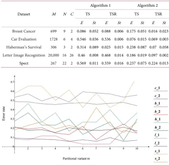
problem. The effectiveness of the algorithms was studied with five databases from the UCI repository; the objects in these databases, the objects had only ca-tegorical features. The characteristics of the bases given in Table 1 that cover rather wide ranges of values for the numbers of objects (267 - 20,000), features (3 - 22) and classes (2 - 26).

The dependencies in (3) and (5) are applicable not only for the TS but also for the TRS. Therefore, we calculated the test error rate, fc, and the training error

rate, fl. All the calculations were performed on the basis of the cross-validation

procedure. The database was divided into 10 datasets of approximately equal size. The first 9 datasets were used as the TRS, and the remaining dataset was used for testing. This procedure was applied 10 times. Consequently, for each base, a se-quence of 10 pairs of TRS and TS variants was considered. For each partitioning variant m∈

(

1,10

)

, we calculated the error rates f_сm and flm.

The fсm and flm curves for different databases are shown in Figure 2 and

Figure 3, respectively. The graphs are identified by an ordered pair a_b, where a

is the first letter of the database name and b is the algorithm identifier. For these rates, the average values E and the standard deviations St are given in Table 1.

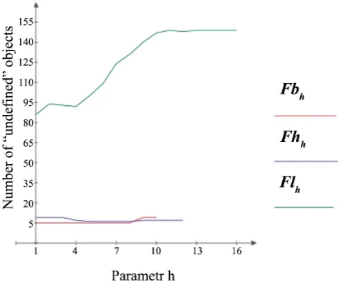
[image:8.595.207.538.386.707.2]

Database Car evaluation and Spect have no “undefined” objects; for them, the functions F h

( )

were not calculated. Figure 4 depicts the curves Fb Fhh, h and

Table 1. Table of databases characteristics and calculation results.

Dataset M N C

Algorithm 1 Algorithm 2 TS TSR TS TSR E St E St E St E St

Breast Cancer 699 9 2 0.086 0.052 0.088 0.006 0.175 0.051 0.016 0.023

Car Evaluation 1728 6 4 0.546 0.036 0.536 0.006 0.076 0.015 0.069 0.003

Haberman’s Survival 306 3 2 0.314 0.089 0.025 0.015 0.238 0.087 0.07 0.058

Letter Image Recognition 20,000 16 26 0.46 0.008 0.468 0.014 0.186 0.019 0.097 0.002 Spect 267 22 2 0.569 0.011 0.559 0.016 0.237 0.075 0.224 0.013

(9)

[image:9.595.212.538.72.255.2]

Figure 3. Frequency distributions of learning errors flm for algorithms 1 and 2.

Figure 4. Graphs of the function F h

( )

for Breast Cancer, Haberman’s Survival and

Letter Image databases.

h

Fl that reflect the features of these functions for the Breast Cancer, Haber-man’s Survival and Letter Image databases, respectively.

Below, we summarize the main results of the calculations:

1) With some exceptions, the error rate curves do not undergo drastic changes under the sequential changes in the composition of the TRS and TS objects un-der cross-validation. Both algorithms yield fairly stable results: in most cases, the error variances for TS and TRS are relatively small (St E<1). The most stable

results were obtained for algorithm 2, where St E<0.4 for the TS. We note that

[image:9.595.251.496.292.495.2]

(10)

con-DOI: 10.4236/jilsa.2019.114004 74 Journal of Intelligent Learning Systems and Applications

sidering the pairwise frequencies of attributes makes it possible to more accu-rately differentiate the latent properties of objects of different classes. For algo-rithm 2, the minimum values of the mean error E are 0.076 and 0.016 for the test and training samples, respectively.

3) In many cases, the introduction of the function F h

( )

and a correspond-ing reduction in the number of “uncertain” objects can lead to significant in-creases in the efficiency of the MPF and in the accuracy of the solution.

We can conclude that these experiments confirm the operability of both algo-rithms.

5. Conclusions

The paper proposes two new algorithms based on the MI for classifying objects with categorical features. Both algorithms originate from the same assumption: that the objects in each class differ in attribute probability distribution, but both algorithms use different models to approximate the distributions. Under this as-sumption, an object class is defined by the individual frequencies of its attribute values rather than by the nonlinear functions of attributes values used in most existing methods. This characteristic explains the comparative simplicity of the proposed algorithms.

It has been established that along with the correlation between categorical attributes, for objects belonging to one class, a functional relationship exists be-tween the attribute values, which is characterized by the frequencies of the pair-wise attribute values. This set of frequencies forms an MPF, which is calculated for the TRS objects for each class and attribute. In one of the algorithms, the MPF is used in conjunction with an analog of the k-nearest neighbors method. This addition allows one to determine the class of a TS object when the TRS does not contain objects with the same combination of attribute values.

It can be expected that the MPF can also be applied to solve problems with quantitative attributes because the values (with some error) can be represented by integers corresponding to the data description with a coarser measuring scale. An experimental examination has shown that algorithm 2, using the MPF, provides more reliable results than does algorithm 1.

Conflicts of Interest

The author declares no conflicts of interest regarding the publication of this pa-per.

References

[1] Bishop, C. (2006) Pattern Recognition and Machine Learning. Springer, Berlin, 738. [2] Hastie, T., Tibshirani, R. and Friedman, J. (2009) The Elements of Statistical

Learn-ing: Data Mining, Inference, and Prediction. 2nd Edition, Springer, Berlin, 764. [3] Murphy, K. (2012) Machine Learning. A Probabilistic Perspective. MIT Press,

(11)

DOI: 10.4236/jilsa.2019.114004 75 Journal of Intelligent Learning Systems and Applications [4] Shats, V.N. (2017) Classification Based on Invariants of the Data Matrix. Journal of

Intelligent Learning Systems and Applications, 9, 35-46. https://doi.org/10.4236/jilsa.2017.93004

[5] Shats, V.N. (2018) The Classification of Objects Based on a Model of Perception.

Studies in Computational Intelligence, 736, 125-131. https://doi.org/10.1007/978-3-319-66604-4_19

[6] Zadeh, L. (1979) Fuzzy Sets and Information Granularity. In: Gupta, N., Ragade, R. and Yager, R., Eds., Advances in Fuzzy Set Theory and Applications, World Science Publishing, Amsterdam, 3-18.

[7] Hogg, R.V., Tanis, E.A. and Zimmerman, D. (2015) Probability and Statistical Infe-rence. 9th Edition, Pearson, London, 557.