Content based media processing

A dissertation submitted to the University of Dublin for the degree of Doctor of Philosophy

Deirdre O’Regan

University of Dublin, Trinity College, April 2010

I hereby declare that this thesis has not been submitted as an exercise for a degree at this or any other University and that it is entirely my own work.

I agree that the Library may lend or copy this thesis upon request.

Signed,

Deirdre O’Regan

This thesis is concerned with Content-Based Media Processing (CBMP). CBMP in-volves the detection or exploitation of the salient content in digital media for applications in digital media processing. Salient content is defined as any attribute, object or “event” that is meaningful, recognizable or important to the user and/or application. The useful-ness of CBMP is explored in three different projects in audio, image and video processing respectively.

The first audio-based project proposes a new algorithm for example-based Sound Tex-ture Synthesis (STS). STS is the synthesis of a long body of sound texTex-ture from a short training example clip. The goal is that the resulting sound texture is perceptually similar to the training example, but does not sound like the training example repetitively tiled. Ap-plications include damaged audio repair, and the generation of ambient sound for computer games, installations and movies. Example-based STS is content-based in that it involves estimating the statistics of the sound texture by measuring directly from the training data. A multi-resolution approach is taken here, and employment of the Dual-Tree Complex Wavelet Transform (DT-CWT) is found to be useful for complexity reduction. Content-based analysis is used for estimating the values of parameters inherent to the algorithm. This example-based STS algorithm performs well compared to another prominent algo-rithm in the field, and the resulting sound textures are of good quality and long duration, temporally varied and perceptually similar to the training example clips tested.

The second image-based project is concerned with Implicit Spatial Inference (ISI) with sparse local features for Face Detection. Face Detection is an extremely important tool in the field of CBMP, since the faces of people constitute much of semantic content in home movies and digital images, cinema and camera mobile phone clips. General Object Detection is also useful, and the use of sparse local features such as SIFT (Scale Invariant Feature Transform) is a popular approach in the field. Linking these sparse features together to properly localize objects, however, is a difficult problem. ISI is a novel technique for leveraging the implicit geometric context of these sparse features in a Bayesian framework. A likelihood is determined from the classification output of a machine learning algorithm trained on these features, and a Markov Random Field (MRF) prior is used to inject contextual geometrical information. The MRF is imposed on a graph obtained by Delaunay triangulation of the sparse features. Promising detection, segmentation and invariance results are obtained in a Face Detection task.

First and foremost I would like to thank my supervisor Prof. Anil Kokaram, for all of his help, encouragement and support over the last four years. Many thanks also to Dr. David Corrigan and Dr. Francois Piti´e for their immediate, generous and invaluable help and advice, especially during the last crucial months.

Thanks to all past and present members of the Sigmedia research group, and staff of the Electronic and Electrical Engineering Department. I particularly wish to thank Dr. Linda Doyle, Dr. Rozenn Dahyot, Dr. Naomi Harte, Prof. Frank Boland and Liam Dowling for their support and kindness over the years. Thanks also to Daire, Hugh, Riccardo, John, Gary and Darren for good memories.

Best of luck to the three other members of the thesis-writing support group! Dan Ring, here’s to eight great years of friendship, adventures, and Italo! Gav Kearney, you’re the best friend that anybody could wish for - rock on! Damien Kelly, you helped get me through with the supportive chats and empathy!

My research has been financed by the Irish Research Council for Science, Engineering and Technology (IRCSET) under the Embark Initiative, and I am very grateful for this funding. Some of this work was also financed by, and carried out at Adobe Systems In-corporated. Thanks to everybody at Adobe for a great summer spent interning in Seattle, most especially Dave Simons and Dr. Andy Moorer.

Contents v

List of Acronyms ix

1 Introduction 1

1.1 Content-Based Media Processing . . . 2

1.2 Thesis Outline . . . 3

1.3 Contributions of this Thesis . . . 4

1.4 Publications . . . 5

2 Example-Based Sound Texture Synthesis 7 2.1 Sound Texture Synthesis . . . 7

2.2 Wavelet Analysis . . . 9

2.3 The Wavelet-Based STS of Dubnov et al. . . 10

2.4 On the Synthesis of Image Texture . . . 12

2.4.1 Thoughts on a Multi-Resolution Example-Based STS . . . 13

2.5 Single Resolution Example-Based Sound Texture Synthesis . . . 14

2.6 The Dual-Tree Complex Wavelet Transform . . . 16

2.7 Multi-Resolution Example-Based Sound Texture Synthesis . . . 17

2.8 Dubnov et al. Training Examples and Sound Textures . . . 22

2.8.1 Comparative Results . . . 23

2.8.2 Subjective Listening Test . . . 26

2.8.3 Observations Concerning Parameters . . . 30

2.9 Content-Based Parameter Estimation . . . 30

2.9.1 Choosing the DT-CWT Level . . . 31

2.9.2 Choosing the Temporal Extent of the Sampling Window . . . 33

2.10 Further Experiments . . . 36

2.10.1 Discussion . . . 37

2.11 Future Work . . . 43

2.12 Conclusion . . . 44

3 Implicit Spatial Inference with Sparse Local Features for Face Detection 46

3.1 Face Detection Explained . . . 47

3.2 Face Detection Algorithms . . . 47

3.2.1 The Viola-Jones Face Detector . . . 48

3.2.2 Rotation and Pose Invariance . . . 50

3.3 Observations on Face Detection . . . 51

3.4 Object Detection . . . 52

3.4.1 SIFT Features . . . 53

3.4.2 Geometric Contexts . . . 55

3.5 Observations on Object Detection . . . 59

3.6 Motivations for Improvement in Face and Object Detection . . . 60

3.7 Implicit Spatial Inference . . . 61

3.7.1 The Bayesian Framework . . . 61

3.7.2 Obtaining the Likelihood . . . 63

3.7.3 The Prior . . . 65

3.7.4 Computing the Posterior Energy . . . 67

3.7.5 Final Rough Segmentation . . . 68

3.8 Testing the ISI Framework . . . 68

3.8.1 Training . . . 71

3.8.2 Testing . . . 72

3.8.3 Test Metrics . . . 73

3.8.4 Choosing Parameters . . . 76

3.8.5 Experiment 1 . . . 76

3.8.6 Experiment 2 . . . 80

3.9 Future Work . . . 82

3.10 Conclusion . . . 83

4 On the Stylization of Visual Media 87 4.1 NPR in Context . . . 87

4.2 SBR Explained . . . 89

4.3 Brush Stroke Attributes . . . 89

4.3.1 Stroke Distribution Mechanisms . . . 91

4.3.2 Stroke Dimensions . . . 97

4.3.3 Stroke Color . . . 99

4.3.4 Stroke Orientation . . . 99

4.3.5 Other Stroke Attributes . . . 100

4.3.6 Ordering . . . 101

4.4 Extending Stylization Effects to Video . . . 102

4.4.2 Temporal Coherency and Other Attributes . . . 107

4.5 Semantically-Driven and NPR and SBR . . . 110

4.6 Motivations for a New NRP/SBR Algorithm . . . 110

5 Graph Cut-Based Skin Detection 114 5.1 On Skin Detection . . . 114

5.2 A New Graph Cut-Based Skin Detector . . . 116

5.2.1 The Bi-Gaussian Likelihood Model . . . 116

5.2.2 A Bayesian Approach . . . 118

5.2.3 The Prior . . . 118

5.2.4 Graph Cut-Based Optimization . . . 118

6 Skin-Aware Stylization of Video Portraits 122 6.1 The Stylization Framework . . . 122

6.2 Elliptical Brush Strokes . . . 123

6.2.1 Calculating the Elliptical Stretch and Orientation . . . 125

6.2.2 An Alternative Technique . . . 127

6.3 Probabilistic Stroke Distribution . . . 127

6.3.1 Two-Pass Anchor Point Distribution . . . 134

6.4 Layer-Based Painting . . . 137

6.4.1 Spatio-Temporal Skin and Edge Detection . . . 137

6.4.2 Separate Stylization of Semantic Layers . . . 139

6.4.3 Moving the Strokes . . . 142

6.5 Spatio-Temporal Color-Sampling . . . 147

6.6 Preserving Some High Frequency Information . . . 150

6.7 Finishing Touches . . . 152

6.8 Summary of the Framework . . . 152

6.9 Results . . . 156

6.10 Future Work . . . 160

6.11 Conclusion . . . 160

7 Conclusion 162 7.1 Future Work . . . 163

7.2 Issues with CBMP . . . 164

7.3 Final Remarks . . . 165

A Further Sound Texture Synthesis Results 166

B Parameter Trials in ISI with Sparse Local Features for Face Detection 170

2D 2-Dimensional

3D 3-Dimensional

B-G Bi-Gaussian

CBMP Content-Based Media Processing

DT-CWT Dual-Tree Complex Wavelet Transform

DWT Discrete Wavelet Transform

EER Equal Error Rate

ICM Iterated Conditional Modes

IIR Infinite Impulse Response

ISI Implicit Spatial Inference

ITS Image Texture Synthesis

MRF Markov Random Field

NPR Non-Photorealistic Rendering

OCD Object Class Detection

PDD Poisson Disk Distribution

PDF Probability Distribution Function

PDS Poisson Disk Sampling

SBR Stroke-Based Rendering

SIFT Scale Invariant Feature Transform

STFT Short-Term Fourier Transform

STS Sound Texture Synthesis

SSD Sum of Square Differences

1

Introduction

With the rise of new digital media formats and ever-evolving digital capture devices, increas-ingly vast quantities of digital media are being produced by everybody from the ordinary digital camera owner to professionals in the broadcasting, cinema, and music industries. This digital revolution has created some very interesting challenges for the contributors and guardians of our technological world.

The problems of finding bandwidth for transmission, and space for storage of both new digital media, and digitized archive material, has fueled the continuous development of increasingly content-basedcompression techniques and summarization schemes. A specific example of such work is the recently popular Seam Carving for Content-Aware Image Resizing algorithm of (Avidan & Shamir, 2007), which is a clever scheme for reducing the size of a digital image by continuously removing “seams” of pixels that snake through the image avoiding thesalient or important image regions. Saliency here is defined by regions of high local contrast or some other measure of importance. A more general example is the huge body of research concerned with the event-based summarization of sporting events for digital TV broadcast, including the research of (Kokaram et al., 2006; Kokaram et al., 2005) and (Denman et al., 2003). It is likely that the producers, broadcasters and owners of digital media will rely increasingly on content-based compression and summarization techniques such as these in the future.

Meanwhile, tools for the manipulation of digital media are extremely popular with both ordinary consumers, and industry professionals. Once based on simple sample-wise, pixel-wise, or frame-wise audio, image, or video processing filters, there is an increasing

demand for smarter media processing tools. Tools that are capable of recognizing, and exploiting knowledge of themeaningful content in digital media, therefore bridging the so-called semantic gap between user and machine. The detection and localization of human faces in visual media for example, has become a hot topic in the field, most probably due to the fact that some of the most important content in home movies, TV broadcasts, and cinema material are captures of people, especially head shots and facial close-ups. Face Detection capability has even found its way into the software bundled with digital cameras and camera mobile phones where it is used to influence functions of the camera such as Auto-Focus (AF).

With the rise of media upload forums such as YouTube1, MySpace2, and Flickr3, any-body can be an audio and/or visual artist. Tools for creative tasks such as image or video stylization and sound editing are becoming as omni-present in ordinary desktop soft-ware as they are in professional media processing softsoft-ware packages such as Adobe Creative Suite4. Time and effort, however, remain precious human commodities and any automation of media processing tasks is invaluable to ordinary consumers, professional media artists, computer game designers, and cinema post-production houses alike.

1.1

Content-Based Media Processing

Content-Based Media Processing (CBMP) involves the detection, analysis or modeling of

the salient content in digital media in order to make decisions based on, or exploit the

content in processing the media. In digital media, salient content can be thought of as any attribute, object or “event” that is semantic, important, recognizable or stand-alone to the user and/or application. There are many different levels of salient or semantic content, some examples of which are listed below:

Low-Level: Local extrema, various local or global statistics (e.g. correlations, entropy), pixelwise color values, motion vectors

Mid-Level: Periodicities (e.g. beats in music), features (e.g. spatial “patches” of image intensity or gradients), relative spatial geometry, properties of a motion field (e.g. occlusion, trajectories)

High-Level: Characteristic color classes (e.g. skin color), semantic events (e.g. goals scored in soccer broadcasts) and objects (e.g. faces)

1_YouTube:

http//www.youtube.com

2_{MySpace: http//www.myspace.com} 3_{Flickr: http//www.flickr.com}

1.2

Thesis Outline

This thesis explores the concept of CBMP in three distinct projects involving audio, im-age and video processing respectively. Each of these projects hinges on the detection or exploitation of some aspect of salient content in a particular topic in media processing. In digital media, salient content can be thought of as any attribute, object or “event” that is semantic, important, recognizable or stand-alone to the user and/or application. Chap-ter 2 describes the audio-based project of example-based Sound Texture Synthesis (STS), Chapter 3 focuses on the image-based project of Implicit Spatial Inference (ISI) with sparse local features for Face Detection, Chapter 4 presents a review of the state-of-the-art in the stylization of visual media, Chapter 5 describes a novel algorithm for Skin Detection in images, and Chapter 6 presents the video-based project entitled Skin-Aware Stylization of Video Portraits. The following is a brief summary of each Chapter.

Chapter 2: Example-Based Sound Texture Synthesis

This Chapter presents a novel example-based Sound Texture Synthesis (STS) algorithm. It begins with an explanation of how the algorithm was inspired by a well known example-based Image Texture Synthesis (ITS) algorithm and its multi-resolution extension. This is followed by a description of the algorithm, including a wavelet-based technique for complex-ity reduction. Next follows a subjective comparison of its sound texture results to those of another prominent wavelet-based STS algorithm. There is a discussion of the meaning and influence of some of the user-defined parameters inherent to the algorithm, along with some suggestions for content-based parameter estimation. Some more interesting sound texture results are then generated using these content-based parameter estimation techniques.

Chapter 3: Implicit Spatial Inference with Sparse Local Features for Face Detection

Chapter 4: On the Stylization of Visual Media

This Chapter presents a review of state-of-the-art algorithms for the artistic stylization of visual media (i.e. images and videos). This includes a description of sub-topics in the field of Non-Photorealistic Rendering (NPR) such as cartoonization, Stroke-Based Rendering (SBR), semantic stylization, motion summarization and expression.

Chapter 5: Graph Cut-Based Skin Detection

This Chapter presents a brief review of techniques in the field of Skin Detection, followed by the description of a novel algorithm for Skin Detection in images. The underlying Bayesian framework of this novel skin detector encompasses probabilistic skin color modeling in the RGB color space and Graph Cut-based spatial smoothing.

Chapter 6: Skin-Aware Stylization of Video Portraits

This Chapter presents a novel Non-Photorealistic/Stroke-based Rendering (NPR/SBR) framework for the skin-aware stylization of video portraits of people. The framework com-bines elements of cartoonization, motion depiction, spatio-temporal Skin and Edge De-tection and content-based stylization. A description of the framework encompasses novel techniques in SBR for brush stroke anchor point distribution and motion expression, spatio-temporal color-sampling, and for the exploitation of occlusion detection in dealing with the well-known issues of gaps and redundancy in motion-compensated brush stroke animation. The framework is used to stylize a number of sequences containing head shots of people, and the visual results are discussed.

Chapter 7: Conclusion

The final Chapter assesses the contributions of this thesis, discusses some issues in CBMP and directions for future work.

1.3

Contributions of this Thesis

The novel aspects of this thesis are summarized as follows

• A new example-based STS algorithm.

• The idea of estimating the parameters inherent to this - and possibly other example-based STS algorithms - through audio content analysis.

• A probabilistic technique for inferring implicit geometric context in sparse local feature-based classification for the purpose of Object/Face Detection.

• A technique for obtaining a probabilistic likelihood from the real-valued confidence output of a typical feature-based machine learning classifier.

• The implementation of ISI on a sparse set of feature points by imposing a MRF via Delaunay triangulation.

• Ideas for producing a rough object segmentation from the final result of sparse local feature-based classification.

• A new probabilistic Skin Detection algorithm with Graph Cut-based spatial smooth-ing.

• A new skin-aware framework for the semantic stylization of video portraits.

• The merging of content-based stylization, cartoonization, SBR, motion summarization and other NPR effects in one video stylization framework.

• Several novel techniques in SBR including a new probabilistic algorithm for brush stroke anchor point distribution, spatio-temporal color sampling, and the detection of video occlusion for the mitigation of some well-known problems in motion-compensated brush stroke animation.

1.4

Publications

Portions of the work described in this thesis have appeared in the following publications

• “Wavelet-Based High Resolution Sound Texture Synthesis”, by Deirdre O’Regan and Anil Kokaram, inProceedings of the 31st International Conference of the Audio Engi-neering Society (AES: Hi-Res Audio ’07): New Directions in High Resolution Audio, paper number 17, Queen Mary University, London, UK, June 2007.

• “Multi-Resolution Sound Texture Synthesis using the Dual-Tree Complex Wavelet Transform”, by Deirdre O’Regan and Anil Kokaram, inProceedings of the 15th Euro-pean Signal Processing Conference (EUSIPCO ’07), pages 350-354, Poznan, Poland, September 2007.

• “Skin-Aware Stylization of Video Portraits”, by Deirdre O’Regan and Anil Kokaram,

in Proceedings of the 6th European IEEE Conference on Visual Media Production

2

Example-Based Sound Texture Synthesis

Sound Texture Synthesis (STS) is useful for synthesizing ambient sounds for installations, computer games and home movies, damaged audio repair, compression and storage. This Chapter presents a novel example-based STS algorithm. A brief examination of some of the concepts in STS and the closely related field of Image Texture Synthesis (ITS) is followed by a description of the new algorithm. Inspired by a well known 2D example-based ITS algorithm and its and multi-resolution adaptation, this 1D audio interpretation is used to synthesize long, perceptually and statistically similar sound textures from much shorter real-world training examples including audio clips of crowd noise, a baby crying, speech and music. The process employs the Dual-Tree Complex Wavelet Transform (DT-CWT) to reduce computational burden without sacrificing spectral coherency in the synthesized audio. This example-based approach to STS produces plausible and interesting sound textures that are comparable to the results of another well-known wavelet-based STS in the field. Content-based analysis of the short training example is used to estimate some of the parameters inherent to the algorithm. Specifically, Beat Detection, and Shannon entropy analysis are used for this purpose.

2.1

Sound Texture Synthesis

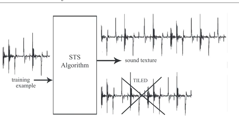
Sound Texture Synthesis (STS) is the automatic synthesis of a long, dynamicsound texture that is perceptually similar to a shorter audio training example, as can be seen in Figure 2.1. The biggest challenge of STS is the achievement of an acoustically plausible sound

STS

Algorithm sound texture

TILED

training example

Figure 2.1: The process of STS; the ideal algorithm takes a short audio training example input and produces a non-tiled sound texture output

texture with an unpredictable temporal evolution. The latter property will be referred to hereafter as variation. Simple end-to-end repetition of the training example, or tiling, is easily detectable acoustically and should be avoided.

A variety of sound samples can be transformed into sound textures; natural (e.g. bab-bling water, crickets chirping), human (e.g. baby crying, speech snippets), musical (e.g. pi-ano), and mechanical (e.g. road traffic). Some natural sounds could be consideredstochastic in nature (e.g. heavy rainfall), whereas human speech and polyphonic music have specific, complex structures, and can be thought of asquasi-periodic. The process of STS is not as easily generalizable as Figure 2.1, since the spectral characteristics of each training example present a unique challenge.

Applications of STS include audio compression, ambient sound or music synthesis for computer games, installations and movies, re-synthesis of rare sounds (e.g. a rare bird call), and error correction or “hole-filling” in existing, damaged audio tracks.

Research in STS is growing in popularity alongside the related fields of Image Texture Synthesis (ITS) and Video Texture. Following the pixel-wise synthesis techniques reported often the field of ITS (e.g. (Efros & Leung, 1999) and (Wei & Levoy, 2000)), STS is taken to mean the sample-wise synthesis of a novel sound track that is much longer than the training example clip. This is subtly different to the idea of Audio Texture (AT) as defined in (Lu et al., 2004), which is concerned with analysis of the training example for location of

transition pointsthat divide the signal into a number of perceptually correlated segments.

STS is also distinct from pure computer music synthesis (Moorer, 1995), which involves the computer-generated composition of virtual, (usually) musical soundwaves without train-ing from any real world audio example clip. Synthesis of complex real-world sounds like human speech is difficult using this technique, but it is useful for creating other-worldly and machine-like sounds such as the THX logo theme, ‘Deep Note’, composed by Dr. J. A. Moorer. For the interested reader, (Strobl et al., 2006) present a short review of a few different methods of sound and music synthesis, including STS, AT and pure computer music synthesis techniques.

With regard to this body of research, the chosen approach of sample-wise STS has been inspired by the interesting results and challenges emerging from the field of ITS in recent years (Efros & Leung, 1999; Wei & Levoy, 2000), with particular regard to multi-resolution or wavelet-optimized ITS algorithms (Wei & Levoy, 2000; Gallagher & Kokaram, 2005). The STS algorithm of (Dubnov et al., 2002) has also been inspired by a multi-resolution ITS algorithm, and it is therefore considered most similar to the STS work presented in this Chapter. This algorithm of (Dubnov et al., 2002), and some ITS algorithms will be discussed later in Sections 2.3 and 2.4 respectively. To fully appreciate this discussion, however, it is necessary to understand the fundamentals of wavelet analysis, and a brief explanation of this topic will now be presented.

2.2

Wavelet Analysis

Wavelet analysis involves the decomposition of a signal into a number of different sub-signals representing the different levels of spectral resolution or scales present in the input signal over time, where scale is inversely proportional to frequency. It is distinct from the Fourier Transform and Short Term Fourier Transform (STFT) in that it results in a non-uniform decomposition of the time-frequency spectrum, as can be seen in Figure 2.2.

Wavelet analysis usually involves filtering the input signal with with a finite energy basis

or mother wavelet function under various translations and dilations. The output wavelet

decomposition is a useful time-scale breakdown of the signal into spectral octaves. For

this reason, wavelet filtering is thought to bear similarity to that of the Human Auditory System (see (Kudumakis & Sander, 1993)), and it is conducive to the spectral analysis of non-stationary, real-world signals.

(a) Fourier analysis (b) STFT analysis

(c) Wavelet analysis

Figure 2.2: Comparing the spectral decomposition of (a) the Fourier Transform, (b) the Short-term Fourier Transform (STFT), and (c) a typical wavelet transform.

granules) of the low frequency bands, which evolve more slowly.

Wavelet transforms are increasingly popular in the field of Texture Synthesis. The DWT is used in (Hoskinson & Pai, 2007) for the location of transition points in AT (see Section 2.1 for explanation). (Hoskinson & Pai, 2007) describe an online demo applet1 _{that can be}

used to experiment with different wavelets basis functions in the creation of a few ambient audio textures such as crickets chirping. The STS and ITS algorithms of (Dubnov et al., 2002) and (Gallagher & Kokaram, 2005) also make use of wavelet transforms for signal analysis, and these will now be discussed in the following two Sections.

2.3

The Wavelet-Based STS of Dubnov et al.

(Dubnov et al., 2002) assume that the short-term time-frequency characteristics of a typical stochastic sound texture can be learned statistically. In similarity to the well-known multi-resolution tree-structured ITS algorithm of (Wei & Levoy, 2000), (Dubnov et al., 2002) perform multi-resolution analysis of the example training clip with the Discrete Wavelet Transform (DWT), and the wavelet decomposition is used to build a tree-like statistical

Figure 2.3: The structure of the nodal wavelet tree used in the STS algorithm of (Dubnov et al., 2002).

model of the training example clip, from which new samples of texture can be continuously drawn.

After wavelet analysis, the training example signal has been broken down intodyadicset of multi-resolution pieces orgranules. These granules are arranged in an inverted tree-like structure with the largest scale (i.e. lowest frequency) granule at the root of the inverted tree, and granules of decreasing scale (i.e. increasing frequency) at descending levels all the way down to the node leaves, which are at the bottom of the tree. As can be seen in Figure 2.3, the structure is arranged such that neighboring nodes at the same tree level are temporally adjacent at the scale represented by that level, whereas parent and child nodes are related in scale-space. The wavelet tree, therefore, models the joint time-scale (i.e. time-frequency) dependencies of the training signal. In (Dubnov et al., 2002), a node’s parents are referred to as its ancestors, whereas its same-level causal neighbors from the past are referred to aspredecessors.

A variety of real-world audio training examples - including traffic noise, babbling water and a baby crying - are re-synthesized, and the resulting sound textures are quite interesting. These results are discussed in further detail in Section 2.8, but a general observation is that the algorithm seems limited to producing sound textures that are of the same, or of even shorter duration than the short example clips used for training. This could be attributed to the fact that the synthesized wavelet trees have only one root node, and are always synthesized to the same depth,K, as that of the training tree. (Dubnov et al., 2002) state that it is a trivial matter to extend the sound texture by means of producing a deeper wavelet tree in synthesis, but this has not been implemented. Both the training examples, and resulting sound texture files are obtainable at the URL associated with (Dubnov et al., 2002)2_.

2.4

On the Synthesis of Image Texture

Most ITS algorithms attempt to generate samples of synthesizedimage textureby modeling

p(I(X)|IΘ), or the likelihood of image intensity,I(X), given some model parameters, IΘ. The well-known algorithm of (Efros & Leung, 1999) was the first in ITS to measure this likelihood directly from the image content, assuming a Markov Random Field (MRF) with a discrete sampling window.

This concept is known asexample-basedsynthesis, and the idea is derived from a statis-tical technique first used by Shannon to generate English-like text letter by letter. Using a large example of training text, Shannon modeled language as a generalized Markov Chain, enabling an estimation of the Probability Distribution Function (PDF) for synthesizing new letters by measuring from the existing data. As discussed in (Efros & Leung, 1999), image texture can be pixel-wise synthesized using this technique adapted to image space. The concept of MRF is explained in (Efros & Leung, 1999) as the assumption that

The probability distribution of brightness values for a pixel given the brightness [i.e. intensity] values of its spatial neighborhood is [assumed to be] independent of the rest of the image.

Unfortunately the window-matching form of this algorithm requires exhaustive searching that is prohibitively slow and computationally inefficient. (Gallagher & Kokaram, 2005) uses wavelet analysis to optimize the ITS algorithm of (Efros & Leung, 1999), reducing the computation burden involved. The Dual-Tree Complex Wavelet Transform (DT-CWT) (Kingsbury, 2001) is used for this task, and the texture synthesis occurs in wavelet space,

as amulti-resolution process. The resulting multi-resolution example-based ITS algorithm

produces image textures that are as plausible as those associated with (Efros & Leung, 1999), but with a fraction of the computational burden. Some of the image texture results

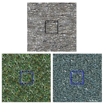
Figure 2.4: Examples of image textures generated by the multi-resolution example-based ITS algorithm of (Gallagher & Kokaram, 2005). Images courtesy of (Gallagher, 2006).

of ITS algorithm of (Gallagher & Kokaram, 2005) can be seen in Figure 2.4. Here, the training example has been placed in the box middle, and the texture is grown outwards from it. The explicit details of this algorithm will not be discussed here, since it is the inspiration behind the example-based STS work that will be described later in this Chapter.

2.4.1 Thoughts on a Multi-Resolution Example-Based STS

Although image and audio are presented and perceived quite differently, it is proposed that example-based STS can be thought of as the 1D version of 2D example-based ITS, and that multi-resolution optimization can be implemented in both. A wavelet-optimized scheme in STS is certainly useful considering the high sampling rate of sound files (e.g. 44kHz or 44,100 samples per second). Sample-wise synthesis in the sound domain, therefore, is even more impractical than in image space.

(Gallagher & Kokaram, 2005) example-based ITS, adapted specifically for the paradigm of audio. The multi-resolution form of this STS algorithm will be discussed later in Section 2.7, in terms of wavelet analysis with the DT-CWT. It is first necessary, however, to understand the 1D case of (Efros & Leung, 1999) example-based texture synthesis algorithm in single resolution.

2.5

Single Resolution Example-Based Sound Texture

Syn-thesis

Suppose that our unit of synthesis,ys, is a single sampleof a body of sound texture. Let Ys be the entire sound texture with N samples to be synthesized from Ye, where Ye is a shorter audio training example of n samples. It is assumed that Ye is long enough to approximate the statistical distribution of the underlying, infinite sound texture from which bothYe andYs are derived. The empty container forYs is initialized by copying a short series of samples, orseed, from Ye to a region in Ys. To interpret the 2D ITS algorithm of (Efros & Leung, 1999) in terms of 1D STS literately, this region would be placed at the mid-point ofYs. This interpretation seems counter-intuitive for audio, however, and so the seed could easily be placed at the beginning ofYs, and therefore the audio will be grown from this seed along the temporal axis in the same direction as time.

Figure 2.5 demonstrates the sample-wise synthesis process. Proceeding from the bound-ary of the seed onwards in time, letys∈Ys be the next sample to be synthesized, and let

w(ys) denote theneighborhoodof samples, encapsulated by a sampling window of temporal extent, Ws, centered on ys. In Figure 2.5, w(ys) is shown as a rectangular window with heavy black outline.

To be able to synthesizeys, it is necessary to create an approximation to the conditional probability distribution,p(ys|w(ys)), determining the likelihood of the amplitude ofysgiven the state of its neighboring samples. In Figure 2.5, the distribution that must be estimated is labeled as PDF for Probability Distribution Function. To create this PDF, a search is conducted to identify all of the neighborhoods in the training example clip, Ye, that are similar in appearance to that defined byw(ys).

Let d(w(ys), w(ye)) represent the perceptual distance between w(ys) and some w(ye), where w(ye) is a neighborhood of extent Ws centered on some sample site ye in Ye. Suppose that the particular w(ye) that is most similar to w(ys) corresponds to wm = MINye∈Ye(d(w(ys), w(ye)). The candidate set, Ω(ys), is constructed such that

Ω(ys) =

(

ye∈Ye, d(ys) =d(w(ys), w(ye)) :d(ys)≤(1 +ǫ)d(w(ys), wm)

)

(2.1)

Figure 2.5: The process of 1D sample-based STS, adapted from the 2D pixel-based ITS algorithm of (Efros & Leung, 1999). Estimating the PDF forp(ys|w(ys)).

create the histogram estimation of the PDF ofp(ys|w(ys)). According to (Efros & Leung, 1999), increasing the value of ǫ is likely to increase the element of variation in the final sound texture, Ys. A value ofǫ > 0 should be chosen to prevent the tiling and repetition of large chunks ofYe inYs. Choosing a value ofǫ= 0 will mostly result in the process of sample-wise copying of Ys from Ye, except when the value of ys has been sampled from the boundary ofYe, in which case variation might be introduced.

In Figure 2.5 depicting this process, Ω(ys) is made up of just three candidates for ys, denoted ye1..3 from Ye, and their perceptual distances from w(ys) are d1..3. In keeping

with (Efros & Leung, 1999), the distanced(w(ys), w(ye)) is defined as the Sum of Square Differences (SSD) as follows

d(w(ys), w(ye)) = Ws X

i=0 GiVi

p

[wi(ys)−wi(ye)]2 Ws

X

i=0 GiVi

(2.2)

emphasize local temporal coherency, and that ofV is to enable “hole-filling” synthesis (i.e. to allow texture to be synthesized where there might be a small hole in the signal). When expressed as a histogram, Ω(ys) is an approximation to the PDF representing p(ys|w(ys)). This histogram can be sampled randomly, yieldingys. This probabilistic sample-wise syn-thesis process can be continued along the axis of time until all of the samples in Ys have been synthesized.

The extent of the sampling window, Ws, is a user-chosen parameter that defines the neighborhood of the implicit MRF, and it is assumed that the PDF is only valid if the extent ofWsis sufficient to capture the underlying statistics ofYe. For best results, therefore, the user must choose a value ofWs to capture the duration of thelongest repetitive temporal

feature in Ye. There is a corresponding, spatial case of this assumption in ITS (Efros &

Leung, 1999). The unit of an audio sample is analogous to that of a pixel for image in the 2D case. Note that the length of the initializing seed must be at least ceil(Ws/2) to ensure a valid synthesis of the first case ofys.

Essentially an exhaustive window-matching algorithm, the computational burden of this process - whether it is used for STS or ITS - is very high. Furthermore, since digital audio is usually sampled at a much higher rate than digital images, the process of STS is extremely computationally inefficient. Drawing inspiration from the multi-resolution example-based ITS of (Gallagher & Kokaram, 2005), a multi-resolution version of this example-based STS has also been developed with the aim of reducing complexity. A brief discussion of Dual-Tree Complex Wavelet Transform (DT-CWT) is now needed, since it is used for wavelet analysis in the multi-resolution extension of example-based STS.

2.6

The Dual-Tree Complex Wavelet Transform

The Dual-Tree Complex Wavelet Transform (DT-CWT) uses a dual tree of wavelet filters to decompose the signal into multi-level wavelet coefficients. The structure of the wavelet decomposition is a coarse-to-fine representation of the spectrum granularity that is most useful for signal analysis and synthesis. At each level,k, the DT-CWT produces a band-pass complex signal ofdetailcoefficients and a low-pass real signal that is passed on to the next level, k+ 1, for further decomposition. This process continues until as many wavelet levels as desired,K, are obtained.

of perfect reconstruction, meaning that no part of the original signal is lost in the inverse wavelet transform.

In contrast to the nodal wavelet tree described in Section 2.3, and the schematic of a wavelet transform seen in Figure 2.2 (c) of Section 2.2, the multi-resolution wavelet decomposition of the DT-CWT is conceptualized as aninverse pyramidal structure in this work, with large-scale coefficients at the bottom, the scales decreasing moving up the levels of the pyramid. Similarly to other wavelet transforms such as the DWT, however, the DT-CWT splits the signal into octaves. It is alsodecimated, and dyadic in structure such that each complex parent coefficient is associated with two complex children at the next wavelet level.

Unlike the DWT, the DT-CWT is shift invariant. Shift invariance means that if the sound samples are shifted within the audio signal undergoing wavelet decomposition, the complex wavelet coefficients undergo the equivalent translation in wavelet space. This property is due to the complex form of the coefficients.

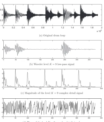
Both the magnitude and phase of the complex coefficients are important metrics in the DT-CWT. Figure 2.6 (a), shows a short drum loop audio sample. After DT-CWT decomposition to level K = 9, Figure 2.6 (b) shows the K = 9 low-pass signal that is representative of the low-frequency information in the signal at that wavelet level. Figure 2.6 (c) is the magnitude (i.e. absolute) of the complex detail signal at level K = 9. In contrast, this captures useful high-frequency information, roughly localizing the onset of the

beatsin the drum loop. Figure 2.6 (d) shows the phase of theK = 9 complex signal, which

is calculated as the inverse tangent of the imaginary divided by real parts of the coefficients of the complex detail signal, resulting in a range of [−π, π] radians. It is important to note that pairs of complex wavelet coefficients can have similar magnitudes, but differing phases, and vice versa. This property is key to the shift invariance, which can be leveraged to promote temporal variation in the wavelet-based STS.

A reduced-complexity multi-resolution version of the example-based STS algorithm de-scribed in Section 2.5 can be formulated by means of a wavelet-optimized synthesis with the DT-CWT. Essentially, sound texture is first synthesized at the largest scale, which represents the coarsestlevel of detail in the signal. Other levels are textured by means of multi-resolution wavelet coefficient transfer. This technique will be discussed in the next Section.

2.7

Multi-Resolution Example-Based Sound Texture

Syn-thesis

0 0.2 0.4 0.6 0.8 1 1.2 1.4 1.6 1.8 2

x 105 −1

−0.5 0 0.5 1

(a) Original drum loop

0 50 100 150 200 250 300 350 400

−5 0 5

(b) Wavelet levelK= 9 low-pass signal

0 50 100 150 200 250 300 350 400

0 2 4 6 8

(c) Magnitude of the levelK= 9 complex detail signal

0 50 100 150 200 250 300 350 400

−4 −2 0 2 4

(d) Phase of the levelK= 9 complex detail signal

Figure 2.6: The DT-CWT of a drum loop to level K = 9; (a) original training example, (b) the finalK= 9 low-pass signal, (c) magnitude of the finalK= 9 complex detail signal, and (d) phase of theK = 9 complex detail signal. The horizontal axis represents sample number[n]. The DT-CWT is decimated so there are fewer samples at wavelet levelK= 9

• A K-level DT-CWT is performed on the short training example clip, Ye, resulting in an inverted pyramid of complex wavelet coefficients,ck_e ∈Ck_e with levelsk= 1..K, where CK

e is the final, coarsest detail signal. A final low-pass residue signal is also produced.

• A multi-level vector space,Ck_s, is initialized to hold the DT-CWT space of the sound texture to be synthesized, Ys. If the target number of texture samples,N, is known in advance, then the extent of these containing vectors can be initialized prior to the synthesis stage. Note that the synthesis, however, is a continuous sample-wise process, such that samples of sound texture can be synthesized ad infinitum if desired. In an application where that would be required, the multi-level containment vectors could simply grow to hold each newly synthesized coefficient at run-time.

• Aseed of samples from the DT-CWT decomposition ofYeis placed in the containing vectors,Ck

s, at each level. This operation is true to the dyadic parent-child structure described earlier in Section 2.6, such that the seed placed inCk_s−1is twice the temporal extent of that placed inCk

s, and symmetrically above it. To adhere to (Efros & Leung, 1999) strictly, the multi-level seed can be placed in the center of any containing vectors, or it may be placed at the beginning of the containers at each level, as can be seen in Figure 2.7. The final level-Klow-pass signal array is also seeded appropriately.

• The sound texture coefficients, ck

s ∈ Cks, must now be synthesized. At the coarsest scale (i.e. level k=K) the single-resolution STS algorithm described in Section 2.5 is used to synthesize the detail coefficients, cK

s ∈CKs . Again, the PDF of each cKs is estimated, and a sample drawn from the candidate set of Ω(cK_s ). Since building this candidate set now involves dealing with complex numbers, Equation 2.2 is modified to the form

d(w(cK_s ), w(cK_e )) = Ws X

i=0 GiVi

p

[Re{wi(cK

s )−wi(cKe )}]2+ [Im{wi(cKs )−wi(cKe )}]2 Ws

X

i=0 GiVi

(2.3)

where are cK_e and cK_s are the complex wavelet coefficients from the final levels, CK_e and CK

• When a cK

s match is placed in CKs , the levels k =K−1..1 are updated in keeping with the parent-child relationship. In other words, the two child coefficients ofcK_s are obtained from those ofcK

e , and so on up the levels of the inverse pyramid. Therefore, when CK_s is fully synthesized, so are all levelsk=K−1..1 above.

• Finally, the synthesized structure is inverse-transformed yielding the longer sound texture, Ys.

Equation 2.3 is similar to the SSD Equation 2.2 used for the case of single-resolution example-based STS (see Section 2.5), except that it has been modified so as to ensure that it is not simply the magnitude of the complex wavelet coefficients that are matched in the SSD, but the real and imaginary parts of the these complex coefficients. This is necessary to preserve the shift invariance property of the DT-CWT in synthesis, and it can have an effect on the statistical variation of the resulting sound texture.

It is also interesting to note that wavelet coefficient matching is not performed at levels above k = K. Instead, the multi-level k = K−1..1 children of the cK

e match for each

cK_s are transferred across to the wavelet space of Ys where they are placed above cKs in the same dyadic pattern as they appear in the wavelet space of Ye. To draw a parallel with the multi-resolution example-based ITS described in (Gallagher & Kokaram, 2005) and (Gallagher, 2006), this technique is known as theCopy variantof the algorithm, because the multi-resolution wavelet coefficients are “copied” to multiple, higher wavelet levels following complex SSD matching at the coarsest level of detail. Other variants of multi-resolution ITS described in (Gallagher, 2006) involvecoarse-to-fine complex SSD matching at decreasing scale levels in wavelet space, and an optimization technique to reduce the complexity of a fully exhaustive search at each level. It was concluded by (Gallagher, 2006), however, that the Copy variant produces results that are comparable to the other multi-resolution synthesis techniques, but with far less computational complexity. A 1D version of the Copy variant is adopted for multi-resolution example-based STS here.

Again, Ws is a user-defined parameter that is chosen to reflect the duration of the longest repetitive temporal feature, but this time with regard to the level-Kcomplex detail signal, CK

e , in the wavelet space of training example Ye. Therefore, the level of DT-CWT decomposition,K, and MRF window size Ws are related. They are complementary variables in that smallerWs is needed to capture the longest repetitive temporal feature in CK_e for largerK.

This multi-resolution example-based STS has a huge computational advantage over the single resolution version of the algorithm described in Section 2.5. The complexity reduc-tion depends on the depth of DT-CWT decomposireduc-tion,K, and corresponding reduction of the sampling neighborhood,Ws. Disregarding the complexity-reducing effect of a shorter

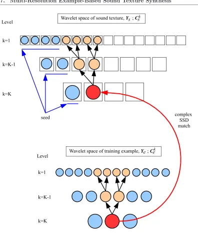
Figure 2.7: Multi-resolution example-based STS; sound texture is grown temporally on-wards from a seed placed in signal containers, Ck_s, initialized to form the wavelet space of the resulting sound texture, Ys. When a complex wavelet coefficient from the coarsest

level, CK_e , of the training example clip, Ye, is chosen by a probabilistic sampling process

it is transfered toCK

s , along with its complex children from levels k=K−1..1

Training Example fs[Hz] t1[s] Description t2d[s]

1 drum loop 22k 3 Near-periodic; percussion with occasional cymbal. 5

2 baby crying 11k 13 Quasi-periodic; baby crying, annoying. 11

3 traffic jam 11k 22 Event-on-background; traffic noise with “yelling” 35

and “honking” events.

4 shore splashing 11k 18 Event-on-background; seawater ebbing with 11

“splashing” event.

5 formula 1 11k 16 Event-on-background; F1 cars accelerating with 23

“gear-shifting” event.

Figure 2.8: Description of training examples used, and resulting sound texture durations, t2d, achieved by the wavelet-based STS of (Dubnov et al., 2002). Here t1 are the time durations of the original training example clips. The training set and results are obtain-able at the URL associated with (Dubnov et al., 2002), and also included on the DVD accompanying this thesis.

This wavelet-based STS algorithm is distinct from that of (Dubnov et al., 2002) in that only temporal predecessors are involved in wavelet coefficient matching, and not hierarchical ancestors (see Section 2.3 for explanation). It is therefore interesting to compare the sound texture results of this multi-resolution STS algorithm with those of (Dubnov et al., 2002) for benchmarking purposes. This comparison will be described in the next Section.

2.8

Dubnov et al. Training Examples and Sound Textures

As discussed in Section 2.3, a number of sound textures were synthesized by the wavelet-based STS of (Dubnov et al., 2002) from a selection of real-world training example clips. These training example clips, their sampling rates,fs, original time durations, t1, and the

durations of the sound textures created by (Dubnov et al., 2002), t2d, are listed in Table

2.8. It is clear that some of the sound textures are actuallyshorter in duration than their corresponding training example clips, which is strange considering the goal of creating a sound texture of extended duration. Other goals in STS are the avoidance or undesirable tiling of the training clip, looping, and uncomfortable glitch-like artifacts known asclicks.

The (Dubnov et al., 2002) textures of training examples 1, drum loop, and 2, baby crying, are interesting, but they contain a clicks, glitches and somewhat erratic variation. The texture of 3, traffic jam, has short, repetitive loops, separated with abrupt silences. The latter effect could occur because a period of recorded silence at the start of the training example clip. Although generally plausible, the domineering presence of long-term car-horn “honking” is not reflected well in the synthesized texture.

of sound signals with both long-term patterns, and sporadic short-term events. These sound phenomena will be referred to as event-on-background signals hereafter. Example

4, shore splashing, is in this category. It sounds like the relaxed tempo of water ebbing

on a shore, punctuated with stochastic-sounding “splashing” events. (Dubnov et al., 2002) acknowledge an unrealistic “nervous splashing activity” in their resulting sound texture. Example 5, formula 1, presents a similar problem. (Dubnov et al., 2002) state that their sound texture does not reflect a good balance between the so-called “long sound phenom-ena” of gradual engine acceleration and short-term “gear-shifting activity” in this training example. Perhaps this effect is due to the limiting technique of matching a fixed number of multi-level predecessors (i.e. five) when sampling wavelet coefficients from the training example for synthesis (see Section 2.3 for explanation).

Both the training example set and sound texture results produced by this algorithm are obtainable at the URL associated with (Dubnov et al., 2002)3_{, and also included on the}

DVD accompanying this thesis.

2.8.1 Comparative Results

Table 2.9 summarizes an experiment in which the example-based STS algorithm presented in Section 2.7 of this Chapter has been used to produce sound textures from the training example clips used by (Dubnov et al., 2002). These training examples are labeled as Ye hereafter in keeping with the notation of Section 2.7. The values for parameters K, Ws, andǫthat produced the best sound texture results are listed, along with the durations,t2o,

of the best sound textures produced. Both the training example files, and sound texture results are included on the accompanying DVD. Again, it is worth noting that there is no theoretical limit to the number of sound texture samples that can be produced by this algorithm, and the duration of the resultant sound texture is therefore arbitrarily chosen. In this case, the values oft2o have been chosen to be many times longer than the durations, t2d of the sound textures produced (Dubnov et al., 2002) (see Table 2.8).

Extensive trial-and-error experimentation was carried out until the best parameter com-binations were found, which is a fairly time-consuming and arduous task. The third column in Table 2.9 states whether the multi-level seed was placed at the start or in the center of the signal containers initialized for the resulting sound texture, as well as the exact samples of the training clip, and time duration constituting the seed. Note that the number of samples, [nK], is actually the number of wavelet coefficients that were placed in the level-K

complex detail signal, CK

s , in the wavelet space of the sound texture, Ys. The number of wavelet samples placed inCK_s−1..k above are true to the dyadic relationship of the DT-CWT, as previously discussed in Section 2.6. The duration in seconds, [s], however, reflects the approximate time duration of the multi-level seed in the final sound texture,Ys.

Ye Training Example Seed (samples[nK], duration[s]) K Ws ǫ t2o[s]

1 drum loop placed at start (1..125,1.5) 8 41 0.3 63

2 baby crying placed at start (100..170,0.4) 6 23 0.1 73

3 traffic jam placed in center (300..311,0.3) 8 5 0.01 70

4 shore splashing placed at start (400..550,3.5) 8 51 0.1 74

5 formula 1 placed start (200..300,2.3) 8 21 0.1 75

Figure 2.9: Parameter values and time durations,t2o, of the best sound textures achieved by testing the new example-based STS algorithm on the training example clips used in the similar work of (Dubnov et al., 2002). The Seed column records the placement of the seed, number of samples,[nK], placed at levelK in wavelet space, and the equivalent time duration in ordinary sample space,[s]. Recall that there is no theoretical constraint on the duration of sound texture that can be produced by this algorithm, and therefore the values fort2o have been arbitrarily chosen here. The resulting sound texture files are included on the DVD accompanying this thesis.

It is interesting to note that the depth of DT-CWT wavelet decomposition is fairly high when compared with a value of K = 3 that is always used in the example-based ITS algorithm of (Gallagher, 2006). This is intuitive, however, since the sampling rate of digital audio is relatively much higher than that of digital images. The sound textures that were produced in this experiment are generally plausible, longer in duration than those of (Dubnov et al., 2002), and sound smooth, varied, and not tiled.

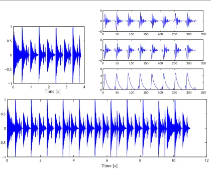
The best sound texture of Ye 1, drum loop, is varied and interesting, with cymbals appearing pseudo-randomly in time. The waveforms of the original training example and 11s of the best sound texture are compared in Figures 2.10 (top right) and (bottom) re-spectively. Visually, the temporal envelope of the sound texture is reminiscent of that of the training example, but it is of much longer duration and well varied. Interestingly, the best performing value for Ws appears to roughly correspond to the tempo of the piece at

K= 8 of the DT-CWT, as can be seen in Figure 2.10 (top left).

A spectrogram (i.e. STFT) of the 13straining example, Ye 2,baby crying, is shown in Figure 2.11 (top left), and the 11ssound texture of (Dubnov et al., 2002) is shown in Figure 2.11 (top right). The first 30s of the best sound texture generated by the new example-based STS algorithm presented here is shown in Figure 2.11 (bottom). The spectral energy of the latter looks natural with regard to the training example clip, and demonstrates good variation. The texture sounds plausible and varied, with very few audible clicks. It is clearly longer, and its spectral envelope looks somewhat more similar to the training example than the sound texture of (Dubnov et al., 2002). All of the spectrograms in Figure 2.11 were created with identical parameters.

0 1 2 3 4 −1

−0.5 0 0.5 1

Time[s_]

0 50 100 150 200 250 300 350 −5

0 5

0 50 100 150 200 250 300 350 −5

0 5

0 50 100 150 200 250 300 350 0

2 4 6

0 2 4 6 8 10 12

−1 −0.5 0 0.5 1

Time[s_]

Figure 2.10: Synthesized drum loop texture; (top left) the 3s training example, Ye 1,

(top right) the real, imaginary, and absolute (t-b) values of the detail coefficients atK= 8

of the DT-CWT ofYe1, and (bottom)11sof the sound texture generated with a1.5sseed,

K= 8,Ws= 41and ǫ= 0.1.

4 andYe5. Specifically, the beginnings and/or ends of these training example clips needed to be cropped to remove small boundaries of recorded silence in the files. It was found that if the silence boundaries are left in Ye, their presence seems to trigger end-to-end tiling of the training example clip in the process of example-based STS if the value of the error metric, ǫ, is not large enough. However, by increasing the value of ǫ, quality is sacrificed in the rest of the sound texture. Some example sound textures resulting from leaving the clips unmodified (i.e. not cropping the silence at the beginning and end) are included on the DVD accompanying this thesis, their parameters listed in Appendix A.

Sample number [n_] F re que nc y [ H z ]

1 2 3 4 5 6 7

x 104 0 0.1 0.2 0.3 0.4 0.5 0.6 0.7 0.8 0.9 1

Sample number [n_]

F re que nc y [ H z ]

1 2 3 4 5 6

x 104 0 0.1 0.2 0.3 0.4 0.5 0.6 0.7 0.8 0.9 1

Sample number [n]

F re q u e n c y [ H z ]

2 4 6 8 10 12 14 16

x 104 0 0.1 0.2 0.3 0.4 0.5 0.6 0.7 0.8 0.9 1

Figure 2.11: Synthesized baby crying texture; (top left) spectrogram of the 13straining example, Ye 2, (top right) the 11s sound texture of (Dubnov et al., 2002), and (bottom) 30s of the sound texture generated by the new example-based STS algorithm with a0.4s seed,K= 6,Ws= 23and ǫ= 0.1.

“nervous”. Figure 2.12 (bottom) shows 25sof the best sound texture produced by the new example-based STS algorithm, which seems more reflective of the ambiance of the training example clip than the sound texture of (Dubnov et al., 2002).

2.8.2 Subjective Listening Test

0 2 4 6 8 10 12 14 16 18 20 −0.6

−0.4 −0.2 0 0.2 0.4

(a) Training exampleYe4,shore splashing

0 2 4 6 8 10 12

−1 −0.5 0 0.5 1

(b) Sound texture generated by (Dubnov et al., 2002)

0 5 10 15 20 25

−0.5 0 0.5

(c) Sound texture generated by multi-resolution STS

Figure 2.12: Synthesized shore texture; (a) training exampleYe 4, (b) the sound texture

generated by the algorithm of (Dubnov et al., 2002), and (c) the sound texture generated by the new example-based STS algorithm with a3.5s seed,K = 8,Ws = 51 and ǫ= 0.1.

Time is measured on the x-axis in seconds[s].

Sound Texture Synthesis (STS) involves the synthesis of a sound texture from a short audio training example clip, such that it sounds natural and varied with regard to, and may be of longer duration than the training example.

Audio clips were played over Genelec 1029A stereo speakers arranged to face the par-ticipants. It was explained to participants that they would hear a short training example clip, followed by two distinct sound texturesA and B. These textures were the results of the two STS algorithms under test. Participants were asked to choose one of the two sound textures with regard to each of the following questions

• Q1Which is more natural with regard to the training example? A or B?

Training example A/B Q1: X/Z Q2: X/Z Q3: X/Z

shore splashing X/Z 0/5 0/5 0/5

baby crying Z/X 0/5 1/4 1/4

drum loop Z/X 0/5 1/4 0/5

traffic jam Z/X 0/5 1/4 0/5

formula 1 X/Z 0/4 2/4 0/5

Figure 2.13: The results of a subjective listening test comparing the STS algorithm of (Dubnov et al., 2002),X, to the new example-based STS algorithm presented here, Z, by asking five participants three questions Q1, Q2 and Q3 gaging which of the two sound textures is preferable. Here, the second column, A/B, lists the order in which the tracks from each algorithm were presented to the listeners (i.e. first played, slash, second played), but the other columns always list the votes for algorithmXversus (i.e. slash) algorithmZ

in that order. The sum of the votes in some columns of the final row do not add up to five. This anomaly is explained in Section 2.8.2.

• Q3Which has better sound quality? A or B?

In these kinds of listening tests the challenge is to guide the listeners to pay attention to the particular sound qualities being examined. Therefore, the meaning of the colloquial terms in the questions were expanded as follows:

• Natural: Sounds like, or has the same “ambiance” and fullness of the spectrum with regard to the training example, contains both long-term and short-term sound “events”.

• Varied: Does not sound like the training example clip on a loop ortiled.

• Sound quality: There are few “clicks” or “glitches”.

An example of a miscellaneous drum loop training example was played on a loop to demonstrate the concept oftiled. Both the order of the five training example clips, and the assignment of A or B to the sound textures of the two STS algorithms were randomized. The participants were allowed to request to hear the training example, sound textures A and/or B as often as required to make a decision, but were not allowed to discuss their deliberations or choices with other participants.

The results of this test are listed in Table 2.13. Each row is representative of a different training example clip and its resultant sound textures (e.g. the sound texture results of

shore splashingare evaluated in the first row). The sound texture result of (Dubnov et al.,

The play order of the two sound textures being compared are separated by a slash (i.e. A/B). In the first row, for example, the column with heading A/B lists the play order as X/Z indicating that sound texture X was played before sound texture Z in this case. The numbers in each column count the number of participants who chose the respective sound texture in response to a particular question, where Q(1-3) are the three questions previously defined. For the results of shore splashing in the first row, in response to Q1, “Which is more natural with regard to the training example?”, 0 listeners preferred sound texture X while 5 preferred sound texture Z.

Overall, participants chose the new example-based STS algorithm presented here over the previous work of (Dubnov et al., 2002). One of the responses to Q1 in row five is not registered because one participant circled both A and B, presumably because it was felt that neither sound texture was preferable with regard to Q1. One particular participant often answered differently in Q2, but in discussions after the test it transpired that this listener was unsure about the explanation of variation as given at the start of the test, deciding that variation meant randomness literally at the sample-level; in other words a very chaotic signal. This outlier serves to highlight how difficult it is to quantitatively assess audio results in terms of subjective phenomena. This is because it is ultimately not possible to equate listening properties in detail between different listeners.

In post-test discussions, participants also revealed that they had been somewhat con-fused by the obvious differences in duration between the two sound textures of each training example. As previously mentioned, some of the sound textures produced by the algorithm of (Dubnov et al., 2002) are so short that they are actually shorter than their corresponding training example clips, whereas those produced by this algorithm are of much longer dura-tion. In their paper, (Dubnov et al., 2002) do not define a sound texture as something that is of longer duration than a training example clip, but given the well known applications of sound texture discussed at the beginning of this Chapter, it is intuitive that extended duration should be a goal in STS. This is another example, however, of the difficulty of quantitatively assessing results and concepts in audio processing.

However, the test performed here does give good evidence that the sound textures produced by this algorithm are plausible and varied with regard to the training example clips, of good quality, and ultimately usable in a media applications. Furthermore, it seems that this STS algorithm is capable of generating natural sound textures from all kinds of training examples with a variety of different spectral profiles. It is capable of dealing with both quasi-periodic and event-on-background training examples which have both long-term, noise-like and short-term, high frequency characteristics in their spectral profiles.

accompanying DVD, their parameters listed in Appendix A.

2.8.3 Observations Concerning Parameters

As previously mentioned, the best parameters for each sound texture were found by virtue of trial-and-error. It soon becomes obvious that choosing too small a value for the extent of the sampling window, Ws, results in the looping of particular small sections of the training example within the sound texture, whereas choosing too large a value causes the phenomenon of tiling. This is becauseWs must be chosen carefully to ensure a valid PDF for each sample with regard to the multi-resolution characteristics of the training example. Choosing too large a value of DT-CWT decomposition level,K, can also result in looping or tiling because the final complex wavelet band CK_e becomes too coarse for a valid PDF. Furthermore, the values ofWs andK are correlated in that the deeper the level of wavelet decomposition,K, the smaller a value ofWsneeded to produce an adequate sound texture. Finally, after choosing values ofWsand K, increasing the value of the error metric,ǫ, past a particular “sweet point” merely results in a clicking and garbled sound texture, again because the PDF becomes invalid.

It was suggested earlier that the sampling window size, Ws, could be related to the tempo of the training example at DT-CWT decomposition level,K. The best sound texture of training example Ye 1, drum loop, for example, was produced with Ws = 41 at level

K = 8. This window size seems to roughly correspond with the spacing of the peaks seen in the level K = 8 wavelet decomposition of the signal in Figure 2.10 (b). These peaks are representative of thebeat characteristicsof the signal at that wavelet level. This observation motivates a scheme for estimating the values of certain parameters within the multi-resolution STS framework through content-based analysis of the training example signal,Ye.

2.9

Content-Based Parameter Estimation

K should result in a fairly coarse complex detail signal at level K, that still retains some characteristic periodicity andsalient detail features.

2.9.1 Choosing the DT-CWT Level

Shannon entropy is a measure of the information content of a signal. The entropy,H, of a signalX is defined as

H(X) =−

m

X

i=1

p(xi) log2p(xi) (2.4)

for random variable X with m outcomes {xi : i = 1, .., m}, and p(xi) is the Probability Distribution Function (PDF) of these xi. In its simplest incarnation, the PDF can be expressed as a normalized m-bin histogram of the xi. A low value of Hk implies a near-random signal with little periodicity and few informative or salient detail features. It is this observation that leads to a method of choosing a good value for the depth of DT-CWT decomposition,K, with regard to the training exampleYe.

Figure 2.15 (a), is 4sof a typical event-on-background training example clip of crowd chatter. This signal contains both noise-like characteristics from the general chat of the crowd watching a game at a baseball stadium, overlaid with event-like bursts of speech from one particular male speaker who can be heard over the background noise. Figure 2.14 (b) plots the Shannon entropy values,Hk =H(Ck_e), of the band-pass complex detail signals,Ck

e, from levelsk= 1..10 of the DT-CWT decomposition of this sound sample. The PDF in this measurement (see Equation 2.9.1) is estimated by a normalized histogram of the absolute values of the complex wavelet coefficients inCk

e from each level k.

The value at zero in this graph is the Shannon entropy of the 4saudio signal in ordinary sample space. Note that the entropy, Hk=1, of the k = 1 detail signal is lower than that of the original training example marked at Hk=0_{. This is to be expected, since C}k=1

e is merely one level of granularity within the original signal. The entropy values, Hk=1..10, of the complex detail wavelet levelsCk=1..10

e seem to increase steadily to a high point at level

k= 7 before suddenly dipping at level k= 8. This seems intuitive since each further level of the wavelet decomposition should reveal salient granules at increasingly coarse wavelet levels. However, the resolution should become too coarse at a certain depth of DT-CWT decomposition to retain the sharp, event-like detail features - such as those constituting the man talking event in thecrowd chattertraining example seen in Figure 2.14 (a) - and this explains the dip in entropy seen Figure 2.14 (b).

0 0.5 1 1.5 2 2.5 3 3.5 4 −0.2

−0.15 −0.1 −0.05 0 0.05 0.1 0.15 0.2 0.25

Time [s]

(a) Event-on-background crowd chatter

0 1 2 3 4 5 6 7 8 9 10

0 0.5 1 1.5 2 2.5 3

k

H

(b)Hk _{measured at each level of the DT-CWT}

Figure 2.14: Choosing the DT-CWT level, K; (a) example training clip of event-on-background crowd chatter, and (b) the process of choosing K by analyzing the Shannon entropy of the absolute of thek-level complex detail signals. AK= 7 DT-CWT decompo-sition is deemed acceptable with regard to the criterion presented in Equation 2.5.

Hk+1 > Hk⇒k=k+ 1 ,Hk+1 ≤Hk⇒k=K (2.5)

The entropy in Figure 2.14 (b) dips in wavelet space for the first time atk= 8. There-fore, using this scheme, levelK = 7 would be chosen as the depth of DT-CWT for multi-resolution STS with thecrowd chattertraining example analyzed in Figure 2.14.

prediction from Equation 2.5 is found to perform well.

Furthermore, note that the entropy in Figure 2.14 (b) rises again afterk= 8. There are also points in this plot at which Shannon entropy is ill-defined, such as atk= 10. Equation 2.5 may not be the optimal criterion for entropy analysis, but it is certainly useful for an initial guess that can be refined if an adequate sound texture is not produced. Other options for entropy analysis include choosingK as the deepest k > kd with Hk > t, where kd is the DT-CWT level at which Hk dips for the first time (e.g. k = 8 in the case of Figure 2.14 (b)), andt is a threshold on the minimum entropy allowed. A visual inspection of the behavior ofHkfor multiple levels of DT-CWT decomposition can also be useful in choosing the value ofK.

2.9.2 Choosing the Temporal Extent of the Sampling Window

Recall from Section 2.7 that the temporal extent of the sampling window, Ws, should be chosen to reflect the longest repetitive temporal feature inCK_e . Figure 2.15 (b) shows C_eK

from the 10-level DT-CWT of a training example ofpolyphonic music seen in Figure 2.15 (a). It is clear to see that the salient quasi-periods of the music appear to be encoded in

thepeaksof CK

e . In the case of a musical signal, these peaks usually represent beats, such as the ones played by the drummer in a band. The tempo of the piece is defined by the spacing of the beats, or the beat period. If it can be assumed that many quasi-periodic sound examples have some sort of tempo - albeit erratic in the case of natural sounds such as human laughter, water splashing, or event-on-background signals - then perhaps the most suitable value of Ws could be estimated as a multiple of the dominant beat period. This is certainly plausible in the case of musical signals such as the polyphonic music example seen in Figure 2.15 (a), or thedrum loop training example, Ye 1, shown in Fi