An extended study on predicting team performance
Leandro Soriano Marcolino1 · Aravind S. Lakshminarayanan2 · Vaishnavh Nagarajan3 · Milind Tambe4
Received: date / Accepted: date
Abstract Voting among different agents is a powerful tool in problem solving, and it has been widely applied to improve the performance in finding the correct answer to complex problems. We present a novel benefit of voting, that has not been observed before: we can use the voting patterns to assess the performance of a team and predict their final outcome. This prediction can be executed at any moment during problem-solving and it is completely domain independent. Hence, it can be used to identify when a team is failing, allowing an operator to take remedial procedures (such as changing team members, the voting rule, or increasing the allocation of resources). We present three main theoretical results: (i) we show a theoretical explanation of why our prediction method works; (ii) contrary to what would be expected based on a simpler explanation using classical voting models, we show that we can make accurate predictions irrespective of the strength (i.e., performance) of the teams, and that in fact, the prediction can work better for diverse teams composed of differ-ent agdiffer-ents than uniform teams made of copies of the best agdiffer-ent; (iii) we show that the quality of our prediction increases with the size of the action space. We perform extensive exper-imentation in two different domains: Computer Go and Ensemble Learning. In Computer Go, we obtain high quality predictions about the final outcome of games. We analyze the prediction accuracy for three different teams with different levels of diversity and strength, and show that the prediction works significantly better for a diverse team. Additionally, we show that our method still works well when trained with games against one adversary, but tested with games against another, showing the generality of the learned functions. More-over, we evaluate four different board sizes, and experimentally confirm better predictions in larger board sizes. We analyze in detail the learned prediction functions, and how they
Leandro Soriano Marcolino E-mail: [email protected] Aravind S. Lakshminarayanan E-mail: [email protected] Vaishnavh Nagarajan
E-mail: [email protected] Milind Tambe
E-mail: [email protected]
1Lancaster University, Lancaster, Lancashire, LA1 4WA, United Kingdom 2Indian Institute of Technology Madras, Chennai, Tamil Nadu, 600036, India 3Carnegie Mellon University, Pittsburgh, PA, 15213, USA
change according to each team and action space size. In order to show that our method is domain independent, we also present results in Ensemble Learning, where we make online predictions about the performance of a team of classifiers, while they are voting to classify sets of items. We study a set of classical classification algorithms from machine learning, in a data-set of hand-written digits, and we are able to make high-quality predictions about the final performance of two different teams. Since our approach is domain independent, it can
be easily applied to a variety of other domains.1
Keywords Teamwork·Collective intelligence·Distributed problem solving·Social
choice theory·Single and multiagent learning
1 Introduction
It is well known that aggregating the opinions of different agents can lead to a significant performance improvement when solving complex problems. In particular, voting has been extensively used to improve the performance in machine learning [66], crowdsourcing [55, 4], and even board games [57, 64]. Additionally, it is an aggregation technique that does not depend on any domain, being very suited for wide applicability. However, a team of voting agents will not always be successful in problem-solving. It is fundamental, therefore, to be able to quickly assess the performance of teams, so that a system operator can take actions to recover the situation in time. Moreover, complex problems are generally characterized by a large action space, and hence methods that work well in such situations are of particular interest.
Current works in the multi-agent systems literature focus on identifying faulty or erro-neous behavior [44, 48, 74, 13], or verifying correctness of systems [24]. Such approaches are able to identify if a system is not operating correctly, but provide no help if a correct system of agents is failing to solve a complex problem. Other works focus on team analysis. Raines et al. (2000) [68] present a method to automatically analyze the performance of a team. The method, however, only works offline and needs domain knowledge. Other meth-ods for team analysis are heavily tailored for robot-soccer [69] and focus on identifying opponent tactics [60].
In fact, many works in robotics propose monitoring a team by detecting differences in the internal state of the agents (or disagreements), mostly caused by malfunction of the sensors/actuators [42, 41, 39, 40]. In a system of voting agents, however, disagreements are inherent in the coordination process and do not necessarily mean that an erroneous situation has occurred due to such malfunction. Additionally, research in social choice is mostly fo-cused on studying the guarantees of finding the optimal choice given a noise model for the agents and a voting rule [14, 49, 19], but provide no help in assessing the performance of a team of voting agents.
There are also many recent works presenting methods to analyze and/or make
predic-tions abouthumanteams playing sports games. Such works use an enormous amount of
data to make predictions about many popular sports, such as American football [67, 34], soccer [10, 52] and basketball [53, 51]. Clearly, however, these works are not applicable to analyzing the performance of a team of voting agents.
Hence, in this paper, we show a novel method to predict the final performance (success or failure) of a team of voting agents, without using any domain knowledge. Therefore, our method can be easily applied in a great variety of scenarios. Moreover, our approach can
be quickly applied online at any step of the problem-solving process, allowing a system operator to identify when the team is failing. This can be useful in many applications. For example, consider a complex problem being solved on a cluster of computers. It is unde-sirable to allocate more resources than necessary, but if we notice that a team is failing in problem solving, we might wish to increase the allocation of resources. Or consider a team playing together a game against an opponent (such as board games, or poker). Different teams might play better against different opponents. Hence, if we notice that a team is pre-dicted to perform poorly, we could dynamically change it. Under time constraints, however, such prediction must be done quickly.
Although related, note that the contribution of this paperis notin using a team of
ex-perts to solve a problem or make predictions [15] or aggregating multiple classifiers through voting as in ensemble systems [66]. Our objective is, given a team of voting agents, to make a prediction about such a team, in order to estimate whether they will be able to solve a certain problem or not.
Our approach is based on a prediction model derived from a graphical representation of the problem-solving process, where the final outcome is modeled as a random variable that is influenced by the subsets of agents that agreed together over the actions taken at each step towards solving the problem. Hence, our representation depends uniquely on the coordination method, and has no dependency on the domain. We explain theoretically why we can make accurate predictions, and we also show the conditions under which we can use a reduced (and scalable) representation. Moreover, our theoretical development allows us to anticipate situations that would not be foreseen by a simple application of classical voting theories. For example, our model indicates that the accuracy can be better for diverse teams composed of different agents than for uniform teams, and that we can make equally accurate predictions for teams that have significant differences in playing strength (which is later confirmed in our experiments). We also study the impact of increasing the action space in the quality of our predictions, and show that we can make better predictions in problems with large action spaces.
We present experimental results in two different domains: Computer Go and Ensemble Learning. In the Computer Go domain, we predict the performance of three different teams of voting agents: a diverse, a uniform, and an intermediate team (with respect to diversity); in four different board sizes, and against two different adversaries. We study the predictions at every turn of the games, and compare with an analysis performed by using an in-depth
search. We are able to achieve an accuracy of 71% for a diverse team in 9×9 Go, and
of 81% when we increase the action space size to 21×21 Go. For a uniform team, we
obtain 62% accuracy in 9×9, and 75% accuracy in 21×21 Go. We also show that we are
still able to make high-quality predictions when training our prediction functions in games against one adversary, but testing them in games against another adversary, demonstrating their generality.
We evaluate different classification thresholds usingReceiver Operating Characteristic
different board sizes. Our analysis shows that the functions are not only highly non-trivial, but in fact even open new questions for further study.
In the Ensemble Learning domain, we predict the performance of classifiers that vote to assign labels to set of items. We use the scikit-learn’s digits dataset [65], and teams vote to correctly identify hand-written digits. We are also able to obtain high-quality predictions online about the final performance of two different teams of classifiers, showing the appli-cability of our approach to different domains.
2 Related Work
The research outlined in this article is related to several key areas of related work in multi-agent systems and machine learning, including voting, team performance assessment, (hu-man) sports analytics, agent verification, robotics, multi-agent learning, multiple expert sys-tems and ensemble syssys-tems.
We first discuss research in voting. Voting is a technique that can be applied in many dif-ferent domains, such as: crowdsourcing [55, 4], board games [56, 57, 64], machine learning [66], forecasting systems [37], etc. Voting is very popular since it is highly-parallelizable, easy to implement and provide theoretical guarantees. It is extensively studied in social choice. Normally, it is presented under two different perspectives: as a way to aggregate different opinions, where different voting rules are analyzed to verify if they satisfy a set of axioms that are considered to be important to achieve fairness [63]; or as a way to discover an optimal choice, where different voting rules are analyzed to verify if they converge to always picking the action that has the highest probability of being correct [49, 19, 14].
Since the classical works of Bartholdi et al. [7, 8], many works in social choice also study the computational complexity of computing the winner in elections [3, 2], and/or of manipu-lating the outcome of an election, in general by disguising an agent’s true preference [18, 23, 79]. There are also works studying the aggregation of partial [77, 78] or non-linear rankings (such as pair-wise comparisons among alternatives) [25], since it could be costly/impossible to request agents for a full linear ranking over all possible actions. Some very recent works in social choice also analyze probabilistic voting rules, where the agents’ votes affect a probability distribution over outcomes [11, 16].
In this work we present a novel perspective to social choice, as instead of studying the computational complexity of manipulation, or the complexity of calculating the winner and the theoretical guarantees of different voting rules, we show here that we can use the voting
patterns as a way toassess the performanceof a team. Such a “side-effect” of voting has not
been observed before, and was never explored in social choice theory and/or applications. Concerning team assessment, the traditional methods rely heavily on tailoring for spe-cific domains. Raines et al. (2000) [68] present a method to build automated assistants for post-hoc, offline team analysis; but domain knowledge is necessary for such assistants. Other methods for team analysis are heavily tailored for robot-soccer, such as Ramos and Ayanegui (2008) [69], that present a method to identify the tactical formation of soccer teams (num-ber of defenders, midfielders, and forwards). Mirchevska et al. (2014) [60] present a domain independent approach, but they are still focused on identifying opponent tactics, not in as-sessing the current performance of a team.
domains we do not have a model of the capabilities of the agents, and we would have to rely on observing the team to estimate its performance, as we propose in this work.
There is also a body of work that focuses on analyzing (and predicting the performance of)humanteams playing sports games. For example, Quenzel and Shea (2014) [67] learn a prediction model for tied NFL American football games, where they use logistic regression to predict the final winner. They study the coefficients of the regression model to determine which factors affect the final outcome with statistical significance. Heiny and Blevins (2011) [34] use discriminant analysis to predict which strategy an American football team will adopt during the game. In soccer, Bialkowski et al. (2014) [10] analyze data from games to automatically identify the roles of each player, and Lucey et al. (2015) [52] also use logistic regression to predict the likelihood of a shot scoring a goal. We can also find examples in basketball. Maheswaran et al. (2012) [53] use a logistic regression model to predict which team will be able to capture the ball in a rebound, while Lucey et al. (2014) [51] study which factors are important when predicting whether a team will be able to perform an open 3-points shot or not.
In the multi-agent systems community, we can see many recent works that study how to identify agents that present faulty behavior [44, 48, 74]. Other works focus on verifying correct agent implementation [24] or monitoring the violation of norms in an agent system [13]. Some works go beyond the agent-level and verify if the system as a whole conforms to a certain specification [46], or verify properties of an agent system [36]. However, a team can still have a poor performance and fail in solving a problem, even when the individual agents are correctly implemented, no agent presents faulty behavior, and the system as a whole conforms to all specifications.
Sometimes even correct agents might fail to solve a task, especially embodied agents (robots) that could suffer sensing or actuating problems. Kaminka and Tambe (1998) [42] present a method to detect clear failures in an agent team by social comparison (i.e., each agent compares its state with its peers). Such an approach is fundamentally different than this work, as we are detecting a tendency towards failure for a team of voting agents (caused, for example, by simple lack of ability, or processing power, to solve the problem), not a clearly problematic situation that could be caused by imprecision/failure of the sensors or actuators of an agent/robot. Later, Kaminka (2006) [41], and Kalech and Kaminka (2007, 2011) [39, 40] study the detection of failures by identifying disagreement among the agents. In our case, however, disagreements are inherent in the voting process. They are easy to detect but they do not necessarily mean that a team is immediately failing, or that an agent presents faulty behavior/perception of the current state.
This work is also related to multi-agent learning [80], but normally multi-agent learning methods are focused on learning how agents should perform, not on team assessment. An interesting approach has recently been presented in Torrey and Taylor (2013) [76], where they have studied how to teach an agent to behave in a way that will make it achieve a high utility. Besides teaching agents, it should also be possible to teach agent teams. During the process of teaching, it is fundamental to identify when the system is leading towards failure. Hence, our approach could be integrated within a team teaching framework.
different, as we present a technique to predict the final performance of a team of voting
agents. Hence, our contributionis notin using a team of agents to make predictions about
someone else’s performance. We predict the future performance of our own agent team with a domain independent approach, and we do not use ensembles to perform such prediction. We train a single predictor function and run it a single time for each world state where we wish to perform a prediction.
Being able to analyze the performance of a team is, however, also important in the study of ensemble systems. Team formation is also necessary for ensembles, as we should pick the classifiers that lead to the best performance [28]. Hence, the technique introduced in this paper could, in principle, also be applied to make predictions about whether a given ensemble will be successful or not in solving a certain classification task.
Finally, it has recently been shown that diverse teams of voting agents are able to out-perform uniform teams composed of copies of the best agent [56, 57, 38]. Marcolino et al. (2013) [56] show necessary conditions for a diverse team to overcome a uniform team, Mar-colino et al. (2014) [57] study how the performance of these teams change as the action space increases, and Jiang et al. (2014) [38] analyze asymptotic guarantees for such teams under classical social choice models, besides studying the performance of ranked voting rules. The importance of having diverse teams has also been explored in the social sciences literature, for example in the works of Hong and Page (2004) [35], and LiCalzi and Surucu (2012) [47], that study models where agents are able to know the utility of the solutions, and the team can simply pick the best solution found by one of its members. Hence, none of these previous works dealt with learning a prediction model to estimate online whether a certain team will win or lose a given game. Additionally, we present here an extra benefit of having diverse teams: we show that we can make better predictions of the final performance for diverse teams than for uniform teams. We will, however, build on the model of Marcol-ino et al. (2014) when we show that the prediction quality of our technique increases with the action space size.
3 Prediction Method
We start by presenting our prediction method, and in Section 4 we will explain why the method works. We consider scenarios where agents vote at every step (i.e., world state) of a complex problem, in order to take common decisions at every step towards problem-solving.
Formally, letTbe a set of agentsti,Abe a set of actionsajandSbe a set of world statessk.
The agents must vote for an action at each world state, and the team takes the action decided
by theplurality voting rule, that picks the action that received the highest number of votes
(we assume ties are broken randomly). The team obtains a final rewardrupon completing all
world states. In this paper, we assume two possible final rewards: “success” (1) or “failure” (0).
We define the prediction problem as follows: without using any knowledge of the do-main, identify the final reward that will be received by a team. This prediction must be executable at any world state, allowing a system operator to take remedial procedures in time.
action was selected as the action of the team by the plurality voting rule). When learning the prediction function we calculate the feature vector considering the whole history of the problem solving process (for example, from the first to the last turn of a game). When using the learned prediction function to actually perform a prediction, we can simply compute the feature vector considering all history from the first world state to the current one (for example, from the first turn of a game up to the current turn), and use it as input to our learned function. Note that our feature vector does not hold any domain information, and
uses solely thevoting patternsto represent the problem solving instances.
Formally, letP(T) ={T1,T2, . . .}be the power set of the set of agents,aibe the action
chosen in world statesjandHj⊆Tbe the subset of agents that agreed onaiin that world
state. Consider the feature vectorx= (x1,x2, . . .)computed at world statesj, where each
dimension (feature) has a one-to-one mapping withP(T). We definexias theproportion
of times that the chosen action was agreed upon by the subset of agentsTi. That is,
xi=
|Sj|
∑
k=1I(Hk=Ti) |Sj|
,
whereIis the indicator function andSj⊆Sis the set of world states froms1to the current
world statesj.
Hence, given a setXsuch that for each feature vectorxt∈Xwe have the associated
rewardrt, we can estimate a function, ˆf, that returns an estimated reward between 0 and 1
given an inputx. We classify estimated rewards above a certain thresholdϑ (for example,
0.5) as “success”, and below it as “failure”.
In order tolearnthe classification model, the features are computed at the final world
state. That is, the feature vector will record the frequency that each possible subset of agents won the vote, calculated from the first world state to the last one. For each feature vector, we have (for learning) the associated reward: “success” (1) or “failure” (0), accordingly
with the final outcome of the problem solving process. In order toexecutethe prediction,
the features are computed at the current world state (i.e., all history of the current problem solving process from the first world state to the current one).
We use classification by logistic regression, which models ˆf as
ˆ
f(x) = 1
1+e−(α+βββTx),
whereα andβββ are parameters that will be learned givenXand the associated rewards.
While training, we eliminate two of the features. The feature corresponding to the subset /0 is dropped because an action is chosen only if at least one of the agents voted for it. Also, since the rest of the features sum up to 1, and are hence linearly dependent, we also drop the feature corresponding to all agents agreeing on the chosen action.
We also study a variant of this prediction method, where we use only information about the number of agents that agreed upon the chosen action, but not which agents exactly
were involved in the agreement. For that variant, we consider a reduced feature vectory=
(y1,y2, . . .), where we defineyi to be the proportion of times that the chosen action was
agreed upon by any subset ofiagents:
yi=
|Sj|
∑
k=1I(|Hk|=i) |Sj| ,
whereIis the indicator function andSj⊆Sis the set of world states froms1to the current
Agent 1 Agent 2 Agent 3
Iteration 1 a1 a1 a2
Iteration 2 a2 a2 a1
Iteration 3 a1 a2 a2
Table 1: A simple example of voting profiles after three iterations of problem-solving.
{t1} {t2} {t3} {t1,t2} {t1,t3} {t2,t3}
Iteration 1 0 0 0 1 0 0
Iteration 2 0 0 0 1 0 0
Iteration 3 0 0 0 2/3 0 1/3
Table 2: Example of the full feature vector after three iterations of problem solving.
3.1 Example of Features
We give a simple example to illustrate our proposed feature vectors. Consider a team of
three agents:t1,t2,t3. Let’s assume three possible actions:a1,a2,a3. Consider that, in three
iterations of the problem solving process, the voting profiles were as shown in Table 1, where we show which action each agent voted for at each iteration. Based on plurality voting rule,
the action chosen for the respective iterations would bea1,a2, anda2.
We can see an example of how the full feature vector will be defined at each iteration in Table 2, where each column represents a possible subset of the set of agents, and we mark the frequency that each subset agreed on the chosen action. Note that the frequency of the
subsets{t1},{t2}and{t3}remains 0 in this example. This happens because we only count
the subset where all agents involved in the agreement are present. If there was a situation
where, for example, agentt1votes fora1, agentt2votes fora2and agentt3votes fora3, then
we would select one of these agents by random tie braking. After that, we would increase the frequency of the corresponding subset containing only the agent that was chosen (i.e.,
either{t1},{t2}or{t3}).
If the problem has only three iterations in total, we would use the feature vector at the last iteration and the corresponding result (“success” — 1, or “failure” — 0), while learning
the function ˆf(that is, the feature vectors at Iteration 1 and 2 would be ignored). If, however,
we already learned a function ˆf, then we could use the feature vector at Iteration 1, 2 or 3
as input to ˆf to execute a prediction. Note that at Iteration 1 and 2 the output (i.e., the
prediction) of ˆf will be exactly the same, as the feature vector did not change. At Iteration
3, however, we may have a different output/prediction.
In Table 3, we show an example of the reduced feature vector, where the column head-ings define the number of agents involved in an agreement over the chosen action. We con-sider here the same voting profiles as before, shown in Table 1. Note that the reduced rep-resentation is much more compact, but we have no way to represent the change in which specific agents were involved in the agreement, from Iteration 2 to Iteration 3. In this case, therefore, we would always have the same prediction after Iteration 1, Iteration 2 and also Iteration 3.
4 Theory
1 2 Iteration 1 0 1 Iteration 2 0 1 Iteration 3 0 1
Table 3: Example of the reduced feature vector after three iterations of problem solving.
probability distribution function (pdf): that is, given the correct outcome, each agent will have a certain probability of voting for the best action, and a certain probability of voting for some incorrect action. These pdfs are not necessarily the same across different world states
[56]. Hence, given the voting profile in a certain world state, there will be a probabilitypof
picking the correct choice (for example, by the plurality voting rule).
We will start by developing, in Section 4.1, a simple explanation of why we can use the voting patterns to predict success or failure of a team of voting agents, based on classical voting theories. Such explanation will give an intuitive idea of why we can use the voting patterns to predict success or failure of a team of voting agents, and it can be immediately derived from the classical voting models. However, it fails to explain some of the results in Section 5, and it needs the assumption that plurality is an optimal voting rule. Hence, it is not enough for a deeper understanding of our prediction methodology. Therefore, we will later present, in Section 4.2, our main theoretical model, that provides a better understand-ing of our results. In particular, based on classical models we would expect to make better predictions for teams that have a greater performance (i.e., likelihood of being correct). Our theory and experiments will show, however, that we can actually make better predictions for teams that are more diverse, even if they have a worse performance. Moreover, we will also be able to build on our model, in Section 4.3, to study the effect of increasing the action space on the prediction quality.
4.1 Classical Voting Model
We start with a simple example to show that we can use the outcome of plurality voting to predict success. Consider a scenario with two agents and two possible actions, a correct and an incorrect one. We assume, for this example, that agents have a probability of 0.6 of voting for the correct action and 0.4 of making a mistake.
If both agents vote for the same action, they are either both correct or both wrong. Hence,
the probability of the team being correct is given by 0.62/(0.62+0.42) =0.69. Therefore, if
the agents agree, the team is more likely correct than wrong. If they vote for different actions, however, one will be correct and the other one wrong. Given that profile, and assuming that we break ties randomly, the team will have a 0.5 probability of being correct. Hence, the team has a higher probability of taking a correct choice when the agents agree than when
they disagree (0.69>0.5). Therefore, if across multiple iterations these agents agree often,
“Correct Outcome”
Agent 1’s vote Agent 2’s vote ... Agent n’s vote
Fig. 1:“Classical” voting model. Each agent has a noisy perception of the truth, or correct
outcome. Hence, its vote is influenced by the correct outcome.
consider a certain agenttthat has a probability 0.6 of voting for the best action, and let’s say
we are in a certain situation where actiona∗is the best action. In this situation agenttwill
have a probability of 0.6 of voting fora∗.
Therefore, given a voting profile and a noise model (the probability of voting for each action, given the correct outcome) of each agent, we can estimate the likelihood of each action being the best by a simple (albeit computationally expensive) probabilistic inference. Any voting rule is going to be optimal if it corresponds to always picking the action that has the maximum likelihood of being correct (i.e., the action with maximum likelihood of being the best action), according to the assumed noise model of the agents. That is, the output of an optimal voting rule always corresponds to the output of actually computing, by the probabilistic inference method mentioned above, which action has the highest likelihood of being the best one.
If plurality is assumed to be an optimal voting rule, then the action voted by the largest number of agents has the highest probability of being the optimal action. We can expect, therefore, that the higher the number of agents that votes for an action, the higher the prob-ability that the action is the optimal one. Hence, given two different voting profiles with a different number of agreeing agents, we expect that the team has a higher probability of being correct (and, therefore, be successful) in the voting profile where a larger number of agents agree on the chosen action.
We formalize this idea in the following proposition, under the classical assumptions of voting models. Hence, we consider that the agents have a higher probability of voting for the best action than any other action (which makes plurality a MLE voting rule [49]), uniform priors over all actions, and that all agents are identical and independent.
Proposition 1 The probability that a team is correct increases with the number of agreeing agents m in a voting profile, if plurality is MLE.
Proof Leta∗be the best action (whose identity we do not know) andV=v1,v2. . .vnbe the
votes ofnagents. The probability of any actionabeing the best action, given the votes of
the agents (i.e.,P(a=a∗|v1,v2. . .vn)), is governed by the following relation:
P(a=a∗|v1,v2. . .vn)∝P(v1,v2. . .vn|a=a∗)P(a=a∗) (1)
Let’s consider two voting profilesV1,V2, where in one a higher number of agents agree
in the chosen action than in the other (i.e.,mV1>mV2). Letw1be the action with the highest
number of votes inV1, andw2the one inV2.
Without loss of generality (since the order does not matter), let’s reorder the voting
profilesV1andV2, such that all votes forw1are in the beginning ofV1and all votes forw2
are in the beginning ofV2. Now, letVx1andVx2be the voting profiles considering only the
firstxagents (after reordering).
We have thatP(VmV2
1 |w1=a∗) =P(V mV2
2 |w2=a∗), since up to the firstmV2agents for
Now, let’s consider the agents frommV2+1 tomV1. InV1, the voted action of all agents
(stillw1) is wired toa∗(by the conditional probability). However, inV2, the voted action
a6=w2 is not wired toa∗ in the conditional probability anymore. As each agent is more
likely to vote fora∗than any other action, frommV2+1 tomV1, the events inV1(an agent
voting fora∗) has higher probability than the events inV2 (an agent voting for an action
a6=a∗). Hence,P(VmV1
1 |w1=a∗)>P(V mV1
2 |w2=a∗).
Now let’s consider the votes aftermV1. InV1there are no more votes forw1, and inV2
there are no more votes forw2. Hence, all the subsequent votes are not wired to any ranking
(as we only wirew1=a∗andw2=a∗in the conditional probabilities). Therefore, each vote
can be assigned to any ranking position that is not the first. Since the agents are independent,
any sequence of votes will thus be as likely. Hence,P(V1|w1=a∗)>P(V2|w2=a∗).
Since we assume uniform priors, it follows that:
P(w1=a∗|V1)>P(w2=a∗|V2)
Therefore, the team is more likely correct in profiles where a higher number of agents
agree.
Hence, if across multiple voting iterations, a higher number of agents agree often, we can predict that the team is going to be successful. If they disagree a lot, we can expect that they are wrong in most of the voting iterations, and we can predict that the team is going to fail.
In the next observation we show that we can increase the prediction accuracy by know-ing not only how many agents agreed, but also which specific agents were involved in the agreement. Basically, we show that the probability of a team being correct depends on the agents involved in the agreement. Therefore, if we know that the best agents are involved in an agreement, we can be more certain of a team’s success. This observation motivates the use of the full feature vector, instead of the reduced one.
Observation 1 Given two profilesV1,V2with the same number of agreeing agents m, the
probability that a team is correct is not necessarily equal for the two profiles.
We can easily show this with an example (that is, we only need one example where the probability is not equal to show that it will not always be equal). Consider a problem
with two actions. Consider a team of three agents, wheret1andt2have a probability of 0.8
of being correct, whilet3 has a probability of 0.6 of being correct. As the probability of
picking the correct action is the highest for all agents, the action chosen by the majority of the agents has the highest probability of being correct (that is, we are still covering a case where plurality is MLE).
However, when onlyt1andt2agree, the probability that the team is correct is given by:
0.82×0.4/(0.82×0.4+0.22×0.6) =0.91. When onlyt2andt3agree, the probability that
the team is correct is given by: 0.8×0.6×0.2/(0.8×0.6×0.2+0.2×0.4×0.8) =0.59.
Hence, the probability that the team is correct is higher whent1 andt2agree than whent2
andt3agree.
However, based solely on the classical voting models, one would expect that given two different teams, the predictions would be more accurate for the one that has greater per-formance (i.e., likelihood of being correct), as we formalize in the following proposition. Therefore, this model fails to explain our experimental results (as we will show later). We
Proposition 2 Under the classical voting models, given two different teams, one can expect to make better predictions for the strongest one.
Proof SketchUnder the classical voting models, assuming the agents have a noise model such that plurality is a MLE, we have that the best team will have a greater probability of
being correct given a voting profile wheremagents agree than a worse team with the same
amount ofmagreeing agents.
Hence, the probability of the best team being correct will be closer to 1 in comparison with the probability of the worse team being correct. The closer the probability of success is to 1, the easier it is to make predictions. Consider a Bernoulli trial with probability of
successp≈1. In the learning phase, we will see many successes accordingly. In the testing
phase, we will predict the majority of the two for every trial, and we will go wrong only
with probability|1−p| ≈0.
Of course, we could also have an extremely weak team, that is wrong most of the time. For such a team, it would also be easy to predict that the probability of success is close to 0. Notice, however, that we are assuming here the classical voting models, where plurality is a MLE. In such models, the agents must play “reasonably well”: classically they are assumed to have either a probability of being correct greater than 0.5 or the probability of voting for the best action is the highest one in their pdf [49]. Otherwise, plurality is not going to be a
MLE.
Consider, however, that the strongest team is composed of copies of the best agent (which would often be the case, under the classical assumptions). We actually have that, in fact, such agents will not necessarily have noise models (pdfs) where the best action has the highest probability in all world states. In some world states, a suboptimal action could have the highest probability, making the agents agree on the same mistakes [56, 38]. There-fore, when plurality is not actually a MLE in all world states, we have that Proposition 1 will not hold in the world states where this happens. Hence, we will predict that the team made a correct choice, when actually the team was wrong, causing problems in our accuracy. We give more details in the next section.
4.2 Main Theoretical Model
We now present our main theory, that holds irrespective of plurality being an optimal voting rule (MLE) or not. Again, we consider agents voting across multiple world states. We as-sume that all iterations equally influence the final outcome, and that they are all independent.
Let the final reward of the team be defined by a random variableW, and let the number
of world states beS. We model the problem solving process by the graphical model in Figure
2, whereHjrepresents the subset of agents that agreed on the chosen action at world state
sj. That is, we assume that the subset of agents that decided the action taken by the team at each world state of the problem solving process will determine whether the team will be successful or not in the end. A specific problem (for example, Go games where the next state will depend on the action taken in the current one) would call for more complex models to be completely represented. Our model is a simplification of the problem solving process, abstracting away the details of specific problems.
For any subsetH, letP(H)be the probability that the chosen action was correct given
the subset of agreeing agents. If the correct action isa∗,P(H)is equivalent to:
P(∀t∈H,tchoosesa∗, ∀t∈/H,tchoosesa6=a∗)
W
H1
H2
H3 H4
. . .
HS
Fig. 2:Our main model. We assume that the subset of agents that decided the action of the
team at each world stateHidetermines whether the team will be successful or not (W).
whereHis the subset of agents which voted for the action taken by the team.
Note thatP(H)depends on both the team and the world state. However, we marginalize
the probabilities to produce a value that is an average over all world states. We consider that,
for a team to be successful, there is a thresholdδ such that:
(
S
∏
j=1P(Hj)
)1/S
>δ (2)
We use the exponent 1/Sin order to maintain a uniform scale across all problems. Each
problem might have a different number of world states; and for one with many world states, it is likely that the incurred product of probabilities is sufficiently low to fail the above test, independent of the actual subsets of agents that agreed upon the chosen actions. However, the final reward is not dependent on the number of world states.
We can show, then, that we can use a linear classification model (such as logistic regres-sion) that is equivalent to Equation 2, to predict the final reward of a team.
Theorem 1 Given the model in Equation 2, the final outcome of a team can be predicted by a linear model over agreement frequencies.
Proof Getting the log in both sides of Equation 2, we have:
S
∑
j=1 1Slog(P(Hj))>log(δ)
The sum over the steps (world states) of the problem-solving process can be transformed
to a sum over all possible subset of agents that can be encountered,P:
∑
H∈PnH
S log(P(H))>log(δ), (3)
wherenHis the number of times the subset of agreeing agentsHwas encountered during
problem solving. Hence, nH
S is the frequency of seeing the subsetH, which we will denote
by fH.
Recall that Tis the set of all agents. Hence, fT (which is the frequency of all agents
agreeing on the same action), is equal to 1−∑H∈P\{T}fH. Also, note thatn/0=0, since at
least one agent must pick the chosen action. Equation 3 can, hence, be rewritten as:
fTlog(P(T)) +
∑
H∈P\T1−
∑
H∈P\{T}fH
!
log(P(T)) +
∑
H∈P\T
fHlog(P(H))>log(δ)
log(P(T)) +
∑
H∈P\T
fHlog
P(H) P(T)
>log(δ)
Hence, our final model will be:
∑
H∈P\Tlog
P(H) P(T)
fH>log
δ P(T)
(4)
Note that log( δ
P(T))and the “coefficients” log(
P(H)
P(T))are allconstantswith respect to a
given team, as we have discussed earlier. Considering the set of all fH(for each possible
subset of agreeing agentsH) to be the characteristic features of a single problem, the
coeffi-cients can now belearnedfrom training data that contains many problems represented using
these features. Further, the outcome of a team can be estimated through a linear model.
The number of constants is exponential, however, as the size of the team grows. There-fore, in the following corollary, we show that (under some conditions) we can approximate well the prediction with a reduced feature vector that grows linearly. In order to differentiate
different possible subsets, we will denote byHia certain subset∈P, and by|Hi|the size
of that subset (i.e., the number of agents that agree on the chosen action).
Corollary 1 If P(Hi)≈P(Hj)∀Hi,Hjsuch that|Hi|=|Hj|, we can approximate the
pre-diction with a reduced feature vector, that grows linearly with the number of agents. Fur-thermore, in a uniform team the reduced representation is equal to the full representation.
Proof By the assumption of the corollary, there is a PH0n, defined asPH0n ≈P(Hj),∀Hj
such that|Hj|=n. Let fn=∑fHj, over all|Hj|=n. Also, letN0be the set of all integers
0<x<N, whereNis the number of agents. We thus have that:
∑
H∈P\TfHlog
P(H) P(T)
≈
∑
x∈N0fxlog
PH0n
P(T)
(5)
AsPH0n depends only on the number of agents, we have that such representation grows
linearly with the size of the team.
Moreover, note that for a team made of copies of the same agent, we have thatPH0n =
P(Hj),∀Hjsuch that|Hj|=n. Hence, the left hand side of Equation 5 is going to be equal
to the right hand side.
Also, notice that our model does not need any assumptions about plurality being an optimal voting rule (MLE). In fact, there are no assumptions about the voting rule at all. Hence, Proposition 1, Observation 1 and Proposition 2 do not apply, and we can still make accurate predictions irrespective of the performance of a team.
We can also note that the accuracy of the predictions is not going to be the same across different teams, and we may actually be able to have better predictions for a lower
perform-ing team. Thelearnedconstants ˆcH≈log(P(H)P(T))represent the marginal probabilities across
Agent State 1 State 2 State 3
Agent 1 a1 a1 a2
Agent 2 a1 a1 a2
Agent 3 a1 a1 a2
Agent 4 a1 a1 a2
(a) Uniform
Agent State 1 State 2 State 3
Agent 1 a1 a1 a2
Agent 2 a2 a2 a1
Agent 3 a3 a1 a3
Agent 4 a3 a1 a2
(b) Diverse
Table 4: An example of a diverse and a uniform team, where we are able to make better predictions for the diverse team.
the agent with the highest marginal probability of voting for the correct choice will not nec-essarily have the highest probability of being correct at all world states. In such world states, the agents tend to agree over the incorrect action that has the highest probability, which will cause problems in our accuracy. Hence, in the following observation, we show that it is pos-sible to make better predictions for a diverse team that has a lower playing performance than a uniform team made of copies of the best agent.
Observation 2 There exists one diverse and one uniform team (made of copies of the best agent), such that the diverse team leads to better prediction accuracy, even though it has a worse playing performance.
We can easily show by an example. Let’s consider the teams shown in Table 4, where each agent has a probability 1 of voting for the action shown in the cell, for each world state.
We consider that the team will be successful when pickinga1, and will fail otherwise. We
assume that one problem solving instance will be consisted by a single world state, which
may be either State 1, State 2 or State 3, each with a 1/3 probability. We also consider that
the teams play by using plurality voting.
Let’s first discuss the uniform team (Table 4 (a)). Given enough training samples, the best predictor that can be created for such team is to predict success when all four agents
agree. However, such predictor will be correct only in 2/3 of the problem instances, as it
will fail in problems consisting of State 3. We can also notice that the uniform team will be
successful in 2/3 of the problem instances.
Let’s consider now the diverse team in Table 4 (b). With enough training samples, the best predictor that can be learned is to predict success when three agents agree, and failure otherwise. This predictor will be correct in all problem instances, even though the team itself
will only be successful in 1/3 of the problem instances.
Although we only give here an existence result, in Section 5 we experimentally show
a statistically significant higher accuracy for the predictions for adiverseteam than for a
uniformteam, even though they have similar strength (i.e., performance in terms of winning
rates). We are able to achieve a better prediction fordiverseteams both in the end of the
problem-solving process and also while doing online predictions at any world state.
4.3 Action Space Size
We present now our study concerning the quality of the predictions over large action space
sizes. In order to perform this analysis, we assume thespreading tail (ST) agent model,
teams of voting agents change in performance as the size of the action space increases. The basic assumption is that the pdf of each member of the team has a non-zero probability over an increasingly larger number of suboptimal actions as the action space grows, while the probability of voting for the optimal action remains unchanged. Marcolino et al. (2014) [57] perform an experimental validation of this model in the Computer Go domain.
For completeness, we briefly summarize here the formal definition of the ST agent
model, and we refer the reader to Marcolino et al. (2014) [57] for a more detailed
descrip-tion. LetDmbe the set of suboptimal actions (aj,j6=0) assigned with a nonzero probability
in the pdf of an agenti, anddm=|Dm|. TheST model assumes that there is a bound in
the ratio of the suboptimal action with highest probability and the one with lowest nonzero
probability, i.e., letpi,min=minj∈Dmpi,jandpi,max=maxj∈Dmpi,j; there is a constantζsuch
thatpi,max≤ζpi,min∀agentsi.STagents are agents whosedmis non-decreasing onmand
dm→∞asm→∞. Marcolino et al. (2014) [57] consider that there is a constantε>0, such
that for allSTagentsi,∀m,pi,0≥ε. They also assume thatpi,0does not change withm.
Let the size of the action space|A|=ρ, andpi,jbe the probability that agentivotes for
action with rank j. Marcolino et al. (2014) [57] show that whenρ→∞, the probability that
a team ofn STagents will play the optimal action converges to:
˜
pbest=1− n
∏
i=1(1−pi,0)− n
∑
i=1(pi,0 n
∏
j=1,j6=i(1−pj,0))
n−1
n , (6)
that is, the probability of two or more agents agreeing over suboptimal actions converges to zero, and the agents can only agree over the optimal choice (note that a suboptimal action can still be taken as we may have situations where no agent agrees). Hence, Equation 6 calculates the total probability minus the cases where the best action is not chosen: the second term covers the case where all agents vote for a suboptimal action and the third term covers the case where one agent votes for the optimal action and all other agents vote for suboptimal actions.
Before proceeding to our study, we are going to make a few definitions and then two
weak assumptions. We consider now here any action space size. Letα be the probability
of a team taking the optimal action when all agents disagree. Since we can only take the
optimal action if one agent votes for that action,αis a function of the probability of each
agent voting for the optimal action. That is, we may have voting profiles where all agents disagree and no agent voted for the optimal action, or we may have voting profiles where all agents disagree, but there is one agent that voted for the optimal action (and, hence, we may still take the optimal action due to random tie braking).
Letβ be the probability of a team taking the optimal action when there is some
agree-ment on the voting profile. β may be different according to each voting profile, but we
assume that we always have thatβ<1 ifρ<∞, andβ=1 ifρ→∞, according to theST
agent model. That is, if two or more agents agree, there is always some probabilityq>0
that they are agreeing over a suboptimal action, andq→0 asρ→∞.
We will make the following weak assumptions: (i) If there is no agreement, the team is
more likely to take a suboptimal action than an optimal action. I.e.,α<1−α; (ii) If there
is agreement, there is at least one voting profile where the team is more likely to take an
optimal action than a suboptimal action. That is, there is at least oneβsuch thatβ>1−β.
Assumption (i) is weak, sinceα<1/n(as we break ties randomly and there may be
cases where no agent votes for the optimal action). Clearly 1/n<1−1/nforn>2.
As-sumption (ii) is also weak, because if we are given a team that is always more likely to take
always outputs “failure” would be optimal (and, hence, we would not need a prediction at all). Therefore, assumption (i) and (ii) are satisfied for all situations of interest. We present now our result:
Theorem 2 LetTbe a set of STagents. The quality of our prediction about the perfor-mance ofTis the highest asρ→∞.
Proof Let’s fix the problem to predicting performance at one world state. Hence, as we
consider a single decision, there is a singleHi such that f
Hi =1, and fHj=0∀j6=i. In
order to simplify the notation, we denote byH the subsetHicorresponding tof
Hi=1. We
also consider the performance of the team as “success” on that fixed world state if they take the optimal action, and as “failure” otherwise.
Let avoting eventbe the process of querying the agents for the vote, obtaining the voting
profile and the corresponding final decision. Hence, it has a unique correct label (“success”
or “failure”). A voting eventξwill be mapped to a pointχin the feature space, according to
the subset of agents that agreed on the chosen action. Multiple voting events, however, will
be mapped to the same pointχ(as exactly the same subset can agree in different situations,
sometimes they may be agreeing over the optimal action, and sometimes they may be
agree-ing over suboptimal actions). Hence, given a pointχ, there is a certain probability that the
team was successful, and a certain probability that the team failed. Therefore, by assigning a label to that point, our predictor will also be correct with a certain probability. With enough data, the predictor will output the more likely of the two events. That is, if given a profile,
the team has a probabilitypof taking the optimal action, andp>1−p, the predictor will
output “success”, and it will be correct with probability p. Correspondingly, if 1−p>p,
the predictor will output “failure”, and it will be correct with probability 1−p. Hence, the
probability of the prediction being correct will be max(p,1−p).
We first study the probability of making a correct prediction across the whole feature space, for different action space sizes, and after that we will focus on what happens with the specific voting events as the action space changes.
Let us start by considering the case whenρ→∞. By Equation 6, we know that every
time two or more agents agree on the same action, that action will be the optimal one. Note that this is a very clear division of the feature space, as for every single point where
|H| ≥2 the team will be successful with probability 1. Therefore, on this subspace we can
make perfect predictions.
The only points in the feature space where a team may still take a suboptimal action are
the ones where a single agent agrees on the chosen action, i.e.,|H|=1. Hence, for such
points we will make a correct prediction with probability max(α,1−α).
Let’s now consider cases with a smaller action space size (i.e.,ρ<∞). Let’s first
con-sider the subspace|H| ≥2. Before, our predictor was correct with probability 1. Now, given
a voting event where there is an agreement, there will be a probabilityβ<1 of the team
tak-ing the optimal action. Hence, the predictor will be correct with probability max(β,1−β),
but max(β,1−β)<1.
Let’s consider now the subspace|H|=1. Here the quality of the prediction depends
onα, which is a function of the probability of each agent playing the best action. On theST
agent model, however, the probability of one agent voting for the best action is independent
ofρ[57]. Hence,αdoes not depend on the action space size, and for these cases the quality
of our prediction will be the same as before. Therefore, for all points in the feature space,
the probability of making a correct prediction is either the same or worse whenρ<∞than
However, that does not complete the proof yet, because a voting eventξ may map to
a different pointχwhen the action space changes. For instance, the number of agents that
agree over a suboptimal action may overpass the number of agents that agree on the optimal
action as the action spaces changes fromρ→∞toρ<∞. Therefore, we need to show that
our prediction will be strictly better whenρ→∞irrespective of such mapping.
Hence, let us now study the voting events. As the number of actions decrease, a certain
voting eventξ whenρ→∞, will map to a voting eventξ0whenρ<∞(whereξ may or
may not be equal toξ0). Letχandχ0be the corresponding points in the feature space forξ
andξ0. Also, letH andH0be the respective subset of agreeing agents. Let’s consider now
the four possible cases:
(i)|H|=|H0|=1. For such events, the performance of the predictor will remain the
same, that is, for both cases we will make a correct prediction with probability max(α,1−
α). Note that this case will not happen for all events, aspi,06→0 whenρ→∞, hence there
will be at least one event where|H| ≥2.
(ii)|H| ≥2,|H0| ≥2. For such events the performance of the predictor will be higher
whenρ→∞, as we can make a correct prediction for a pointχwith probability 1, while for
a pointχ0with probability max(β,1−β)<1.
(iii)|H| ≥2,|H0|=1. This case will not happen under theST agent model. If there
was a certain subsetHof agreeing agents whenρ→∞, when we decrease the number of
actions the new subset of agreeing agentsH0will either have the same size or will be larger.
This follows from the fact that we may have a larger subset agreeing over some suboptimal action when the action space decreases, but the original subset that voted for the optimal action will not change.
(iv)|H|=1,|H0| ≥2. We know that in this caseξ0is an event where the team fails
(otherwise the same subset would also have agreed whenρ→∞). Hence, for 1−α>α
(weak assumption (i)), we make a correct prediction for such case whenρ→∞. When
ρ<∞, we make a correct prediction if 1−β>β.β, however, depends on the voting profile
of the eventξ0. By weak assumption (ii), there will be at least one event where the team
is more likely to be correct than wrong (that is,β >1−β). Hence, there will be at least
one event where our predictor changes from making a correct prediction (whenρ→∞) to
making an incorrect prediction (whenρ<∞).
Hence, for all voting events, the probability of making a correct prediction will either be
the same or worse whenρ<∞than whenρ→∞, and there will be at least one voting event
where it will be worse, completing the proof. Hence,ρ→∞is strictly the best case for our
prediction. As we assume that all world states are independent, ifρ→∞is the best case for
a single world state, it will also be the best case for a set of world states.
5 Results
5.1 Computer Go
We first test our prediction method in the Computer Go domain. We use four different Go software: Fuego 1.1 [26], Gnu Go 3.8 [27], Pachi 9.01 [9], MoGo 4 [30], and two (weaker)
variants of Fuego (Fuego∆ and FuegoΘ), in a total of six different, publicly available,
agents. Fuego is the strongest agent among all of them [56]. The description of Fuego∆
0.0 0.2 0.4 0.6 0.8 1.0
Winning
Rate
9x9 13x13 17x17 21x21 Diverse
Intermediate Uniform
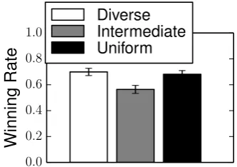
Fig. 3: Winning rates of the three teams, under four different board sizes.
We study three different teams:Diverse, composed of one copy of each agent2;Uniform,
composed of six copies of the original Fuego (initialized with different random seeds, as in
Soejima et al. (2010) [71]);Intermediate, composed of six random parametrized versions of
Fuego (from Jiang et al. (2014) [38]). In all teams, the agents vote together, playing as white, in a series of Go games against the original Fuego playing as black. We study four
differ-ent board sizes fordiverseanduniform: 9x9, 13x13, 17x17 and 21x21. Forintermediate, we
study only 9x9, since the random parametrizations of Fuego do not work on larger boards. In Go a player is allowed to place a move at any empty intersection of the board, so the largest number of possible actions at each board size is, respectively: 81, 169, 289, 441. Computa-tion for the work described in this paper was supported by the University of Southern
Cal-ifornia’s Center for High-Performance Computing (http://hpcc.usc.edu). We ran
the Go games in HP DL165 machines, each with 12 2.33 GHz cores, and 48GB of RAM.
In order to evaluate our predictions, we use a dataset of 1000 games for each team and board size combination (in a total of 9000 games, all played from the beginning). For all results, we used repeated random sub-sampling validation. We randomly assign 20% of the games for the testing set (and the rest for the training set), keeping approximately the same ratio as the original distribution. The whole process is repeated 100 times. Hence, in all graphs we show the average results, and the error bars show the 99% confidence interval
(p=0.01), according to at-test. If the error bars cannot be seen in a certain point in a graph,
it is because they are smaller than the symbol used to mark that point in the graph. Moreover, when we say that a certain result is significantly better than another, we mean statistically
significantly better, according to at-testwherep<0.01, unless we explicitly give apvalue.
First, we show the winning rates of the teams in Figure 3. This result is not yet eval-uating the quality of our prediction, it is merely background information that we will use
when analyzing our prediction results later. On 9x9 Go,uniformis better thandiversewith
statistical significance (p=0.014), and both teams are clearly significantly better than
in-termediate(p<2.2×10⁻¹⁶). On 13x13 and 17x17 Go, the difference betweendiverseand
uniformis not statistically significant (p=0.9619 and 0.5377, respectively). On 21x21 Go, thediverseteam is significantly better thanuniform(p=0.03897).
2 Except for Gnu Go, all other agents use Monte Carlo Tree Search [12]. However, each agent was
In order to verify our online predictions, we used the evaluation of the original Fuego,
but we give it a time limit 50×longer (i.e., it runs for 500sper evaluation)3. We will refer
to this version as “Baseline”. We, then, use the Baseline’s evaluation of a given board state to estimate its probability of victory, allowing a comparison with our approach. Considering
that an evaluation above 0.5 is “success” and below is “failure”, we compare our predictions
with the ones given by the Baseline’s evaluation, at each turn of the games.
We use this method because the likelihood of victory changes dynamically during a game. That is, a team could be in a winning position at a certain stage, after making several good moves, but suddenly change to a losing position after committing a mistake. Similarly, a team could be in a losing position after several good moves from the opponent, but sud-denly change to a winning position after the opponent makes a mistake. Therefore, simply comparing with the final outcome of the game would not be a good evaluation. However, for the interested reader, we show in the appendix how the evaluation would be comparing with the final outcome of the game — and we note here that our prediction quality is still high under that alternative evaluation method.
Since the games have different lengths, we divide all games in 20 stages, and show the average evaluation of each stage, in order to be able to compare the evaluation across all
games uniformly. Therefore, a stage is defined as a small set of turns (on average, 1.35±0.32
turns in 9×9; 2.76±0.53 in 13×13; 4.70±0.79 in 17×17; 7.85±0.87 in 21×21). For
all games, we also skip the first 4 moves, since our baseline returns corrupted information in the beginning of the games.
We will present our results in five different sections. First, we will show the analysis for
a fixed threshold (that is, the valueϑ above which the output of our prediction function ˆf
will be considered “success”). Secondly, we are going to analyze across different thresholds using receiver operating characteristic (ROC) curves, and the area under such curves (AUC). Thirdly, we will present the results for different board sizes. Then, finally, we will study the performance of the reduced feature vector, and we will show results when playing against a different adversary.
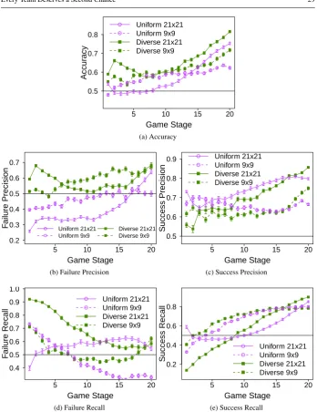
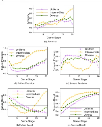
5.1.1 Single Threshold Analysis
We start by showing our results for a fixed threshold, since it gives a more intuitive under-standing of the quality of our prediction technique. Hence, in these results we will consider
that when our prediction function ˆf returns a value above 0.5 for a certain game, it will be
classified as “success”, and when the value is below 0.5, it will be classified as “failure”. In this section we also restrict ourselves to the 9x9 Go case.
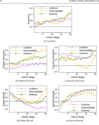
We will evaluate our prediction results according to five different metrics: Accuracy, Failure Precision, Success Precision, Failure Recall, Success Recall. Accuracy is defined as the sum of the true positives and true negatives, divided by the total number of tests (i.e., true positives, true negatives, false positives, false negatives). Hence, it gives an overall view of the quality of the classification. Precision gives the percentage of data points classified
3 As this evaluation is much more computationally expensive than game playing, we allowed it
with a certain label (“success” or “failure”) that are correctly labeled. Recall denotes the percentage of data points that truly pertain to a certain label, that are correctly classified.
We show the results in Figure 4. As we can see, we were able to obtain a high-accuracy
very quickly, already crossing the 0.5 line in the 2ndstage for all teams. In fact, the accuracy
is significantly higher than the 0.5 mark for all teams after the 2ndstage (and fordiverseand
intermediatesince the 1ststage).
From around the middle of the games (stage 10), the accuracy fordiverseanduniform
already gets close to 60% (withintermediateonly close behind). Although we can see some
small drops – that could be explained by the sudden changes in the game –, overall the accuracy increases with the game stage number, as expected. Moreover, for most of the
stages, the accuracy is higher for diversethan foruniform. The prediction fordiverseis
significantly better than foruniformin 90% of the stages. It is also interesting to note that
the prediction forintermediateis significantly better than foruniformin 60% of the stages,
even though intermediateis a significantly weaker team. In fact, we can see that in the
last stage, the accuracy, the failure precision and the failure recall is significantly better for
intermediatethan for the other teams.
5.1.2 Multiple Threshold Analysis
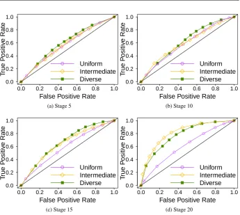
We now measure our results under a variety of thresholds (that is, the valueϑ above which
the output of our prediction function ˆf will be considered “success”). In order to perform
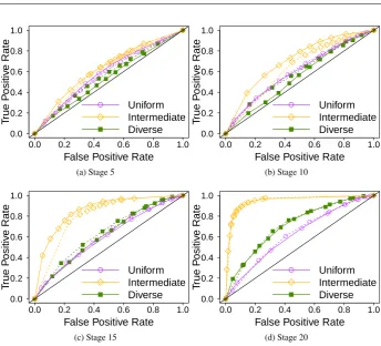
this study, we use receiver operating characteristic (ROC) curves. An ROC curve shows the true positive and the false positive rates of a binary classifier at different thresholds. The true positive rate is the number of true positives divided by the sum of true positives and false negatives (i.e., the total number of items of a given label). That is, the true positive rate shows the percentage of “success” cases that are correctly labeled as such. The false positive rate, on the other hand, is the number of false positives divided by the sum of false positives
and true negatives (i.e., the total number of items thatare notof a given label). That is,
the false positive rate shows the percentage of “failure” cases that are wrongly classified as “success”.
Hence, ROC curves allow us to better understand the trade-off between the true positives and the false positives of a given classifier. By varying the threshold, we can increase the number of items that receive a given label, increasing henceforth the number of items of such label that are correctly classified, but at the cost of also increasing the number of items that incorrectly receive the same label.
The ideal classifier is the one on the upper left corner of the ROC graph. This point (true positive rate = 1, false positive rate = 0) indicates that every item classified with a certain label truly pertains to such label, and every item that truly pertains to such label receives the correct classification.
In this paper, we do not aim only on studying the performance of a single classifier, but rather on comparing the performance of our prediction technique on a variety of situations, changing the team and the action space size (i.e., the board size). Hence, we also study the area under the ROC curve (AUC), as a way to synthesize the quality information from the curve into a single number. The higher the AUC, the better the prediction quality of our technique in a given situation. That is, a completely random classifier would have an AUC of 0.5, and as the ROC curve moves towards the top-left corner of the graph, the AUC gets closer and closer to 1.0.
5 10 15 20 0.5 0.6 0.7 0.8 Game Stage Accur acy ● ● ● ●● ● ● ●● ●● ●● ● ● ●● ●● ● ● Uniform Intermediate Diverse (a) Accuracy
5 10 15 20 0.4 0.5 0.6 0.7 0.8 Game Stage F ailure Precision ● ●● ● ● ● ●● ●● ● ● ●● ● ● ●● ●● ● Uniform Intermediate Diverse
(b) Failure Precision
5 10 15 20 0.4 0.5 0.6 0.7 0.8 Game Stage Success Precision ● ● ●● ● ● ● ● ●● ● ● ●● ● ●● ● ● ● ● Uniform Intermediate Diverse
(c) Success Precision
5 10 15 20 0.3 0.4 0.5 0.6 0.7 0.8 Game Stage F ailure Recall ● ● ● ● ● ● ● ● ●● ● ● ● ● ● ● ● ● ● ● ● Uniform Intermediate Diverse
(d) Failure Recall
5 10 15 20 0.3 0.4 0.5 0.6 0.7 0.8 Game Stage Success Recall ● ● ● ● ●● ●● ● ● ● ● ●● ● ● ● ●● ● ● Uniform Intermediate Diverse
[image:22.595.73.415.69.498.2](e) Success Recall
Fig. 4: Performance metrics over all turns of 9x9 Go games.
correctly considering the item that was truly a “success” as more likely to be a “success” case than the other item. It has also been shown to be related to other important statistical
metrics, such as theWilcoxon test of ranks, theMann-Whitney Uand theGini coefficient
[33, 59, 32].
0.0 0.2 0.4 0.6 0.8 1.0 0.0 0.2 0.4 0.6 0.8 1.0
False Positive Rate
T rue P ositiv e Rate ● ● ● ● ● ● ● ● ● ● ● ● Uniform Intermediate Diverse
(a) Stage 5
0.0 0.2 0.4 0.6 0.8 1.0 0.0 0.2 0.4 0.6 0.8 1.0
False Positive Rate
T rue P ositiv e Rate ● ● ● ● ● ● ● ● ● ● ● ● Uniform Intermediate Diverse
(b) Stage 10
0.0 0.2 0.4 0.6 0.8 1.0 0.0 0.2 0.4 0.6 0.8 1.0
False Positive Rate
T rue P ositiv e Rate ● ● ● ● ● ● ● ● ● ● ● ● Uniform Intermediate Diverse
(c) Stage 15
0.0 0.2 0.4 0.6 0.8 1.0 0.0 0.2 0.4 0.6 0.8 1.0
False Positive Rate
T rue P ositiv e Rate ● ● ● ● ● ● ● ● ● ● ● ● Uniform Intermediate Diverse
[image:23.595.73.419.80.389.2](d) Stage 20
Fig. 5: ROC curves, analyzing different thresholds in 9x9 Go.
there is a clear distinction between the prediction quality fordiverseandintermediate, when
compared with the one foruniform, across many different thresholds.
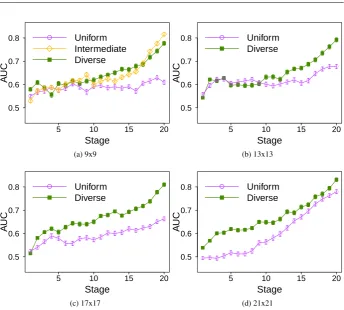
As mentioned, to formally compare these results across all stages we use the AUC met-ric. Hence, in Figure 6, we show the AUC for the three different teams in 9x9 Go. As we can see, the three teams have similar AUCs up to stage 10, but from that stage on we can
get better AUCs for bothdiverseandintermediate, significantly outperforming the AUC for
uniformin all stages. We also find that, considering all stages, we have a significantly better
AUC fordiverse(than foruniform) in 85% of the cases, and forintermediatein 55% of the
cases. Curiously, we can also note that even thoughintermediateis the weakest team, we
can obtain for it the (significantly) best AUC in the last stage of the games, surpassing the AUC found for the other teams. Overall, these results show that our hypothesis that we can make better predictions for teams that have higher diversity holds irrespective of the thresh-old used for classification. On the next section, we study the effect of increasing the action space size.
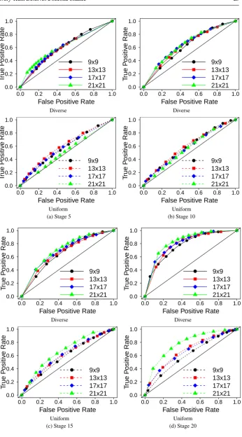
5.1.3 Action Space Size
Let us start by showing, in Figure 7, ROC curves fordiverseanduniformunder different