Abstract— Groundwater salinity is a severe problem particularly to agricultural lands. Measuring the water quality index at some particular locations might not be easy. The objective of this research is hence to predict the groundwater salinity, in terms of electrical conductivity (EC) in the shallow groundwater in the Northeast of Thailand. Groundwater EC was measured for the period of over 2 years at 14 different locations at different time intervals. The data was interpolated and analyzed for basic statistical properties including autocorrelation and stationarity. Linear regression model and transformed linear regression models were developed. The two
models produced high adjusted R2 about 0.8 during the
calibration step. However, the transformed model provided a better accuracy during the verification step. This variation can be attributed to unaccounted factors, collinearity, and stationarity. The model can be applied to predict the groundwater salinity using the groundwater quality measured at some surrounding region.
Index Terms—Multiple regression, groundwater, salinity
I. INTRODUCTION
Salts are natural minerals found underground and can occur in various amount on the top soils. Salts can be harmful to environment and habitat species. Some agricultural productivity can be severely affected by the salty soil and water. Salinity problem in groundwater can be both naturally occurred and human induced. Humans may increase the salinity in the groundwater through the practice of poorly managed irrigation and the excessive use of chemicals. Salts can be dissolved by water since water is the major dissolvent in the natural. Once dissolved in groundwater, saline water will be transported along the groundwater flowpaths and more salts can accumulate more once get into individual flowpaths. The process of capillary rise will bring the saline shallow groundwater to the soil surface and the evaporation process dries the water out leaving the soil with the white crust from salts. Over time, this salt accumulation will lead to soil deterioration and losses in agricultural production.
Groundwater has the ability to demobilize the salts and convey the salty water anywhere the hydraulic gradient of the groundwater leads to. Besides horizontal flow, the saline groundwater can move in vertical direction. The upward movement of saline groundwater is very critical because of
Manuscript received December 7, 2016; revised January 22, 2017. This work was supported in part by the King Mongkut’s Institute of Technology Ladkrabang Research Grant.
U.Seeboonruang is with the Faculty of Engineering, King Mongkut’s Institute of Technology Ladkrabang, Bangkok, 10520, Thailand. (Corresponding author to provide phone: 6681-346-9984; e-mail: [email protected]).
that the salts can endanger the environment. In order to manage the land properly, many questions relating to groundwater and its salinity must be answered and one of this inquiries is the water salinity at specific locations and times. By recognizing and monitoring groundwater movement and quality, lands may be properly managed to help control and diminish such problems. Groundwater may be monitored easily and cheaply through the installation of shallow observation bores. However, measuring water quality continuously requires an extensive amount of time and investment.
Hence, predicting groundwater quality fluctuation over time is vital for appropriate water and land use management. Because of the complicated physics and chemistry in the underground, some mathematical modelling approaches can be too challenging and demanding a lot of input data (Anderson and Woessner 1992), while some numerical methods can be simpler and less time-consuming than others.
Among many different modeling approaches, time series technique is an alternative tool applying to analyze the relationships between different water quality indexes and to predict some unknown parameters. The method is widely used in in other academic research fields, such as economics, hydrology, and biology (Renard 2007; Maiti and Tiwari 2014; Seeboonruang 2014). Another easy method is statistical-based and called multiple linear regression technique. The method is relatively straightforward and less resource consuming. Multiple linear regression modeling has been applied for predicting water quality indexes (Joarder et al. 2008; Agarwal and Agarwal 2013). Hence, this multiple linear regression technique will be applied in this study.
Lower Namkam River Basin is the focus in this study (Fig 1). It is a sub-basin of the Great Mekong River Basin located in the northeast of Thailand. Even though agriculture is the main activity for the local communities in this area, its groundwater is still facing with the problem of salinity. The source of salinity is believed to come from the salt rocks deposited in the past hundred decades. Saline water can be found in the deep aquifers in the study area, while shallow aquifers are locally contaminated. Typically, the deep groundwater is more severe in terms of salinity than the shallow groundwater and there is the upward gradient bringing the saline groundwater to the shallow aquifer (Seeboonruang 2014).
II. METHODOLOGY
A. Data Collection and Preparation
Total of 22 observation wells were installed in the
A Multiple Regression Analysis for Predicting
Salinity in Shallow Groundwater
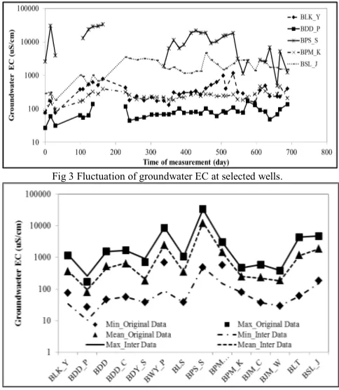
sub-basin. The selection of the locations for these observation wells were based on the previous works and interviews with the locals. The network of observation wells must be distributed over the study area especially in the saline area. Fig 2 shows the locations of these wells. The groundwater EC data was only collected from 14 wells namely BPS_S, BLK, BDD_P, BDD, BDD_C, BDY_S, BWY_P, BLT, BLS, BPMT_D, BPM_K, BJM_C, BJM_W, and BSL_J. The depth of these wells were varied between 4 and 10 m. Groundwater salinity measurement were taken approximately twice a month starting from December 2010 to October 2012. Fig 3 shows the groundwater EC fluctuation over the measuring period. The measurement was performed using the portable Senso Direct Con200. The graph shows that the EC is highly varied on the order of four magnitudes in the basin.
Fig 1 The Lower Nam Kam Basin
Fig 2 Well locations
However, the data collected from the field during the study period was relatively sparse because of the difficulty of accessing the sites and the flood condition.It is necessary to interpolate the EC data into data with identical interval periods. The measured biweekly data was interpolated into daily data using the piecewise linear interpolation (Kumar 2012)
.
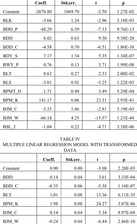
The interpolation refines the sparse data into a set of data with similar spacing, which is required for many time series analysis and regression methods. Fig 4 reveals how the interpolated data honours the original data. The minimum, maximum, and the mean values of both original and interpolated values are significantly analogous.B. Descriptive statistics
Descriptive statistics of the groundwater data is provided by the software, PAST (Paleontological Statistics Software
Package for Education and Data Analysis) (Hammer and Harper 2006; Hammer et al. 2001; Harper 1999). The following values are computed for each set of groundwater data. These numbers are the size of the data, minimum and maximum values, estimate of mean, standard error of the estimate mean, variance, standard deviation, median, 25th and
75th percentiles, skewness, kurtosis, geometric mean, and
[image:2.612.304.546.151.429.2]coefficient of variation.
Fig 3 Fluctuation of groundwater EC at selected wells.
Fig 4 Basic statistical properties between original and interpolated data
C. Stationarization of data
A stationary time series is the statistical property that is required for most statistical forecasting technique. The property refers to the properties of a time series with relatively constant mean, variance, and autocorrelation overtime. Hence, the prediction of the variables in question can be performed based on the fact that their statistical properties remain the same. When the variables in a regression are nonstationary, R square values and t-statistics no longer follow the usual distributions and can be wildly inflated (Granger and Newbold 1974). Two nonstationary time series do not usually maintain their relationship over a long period of time. Hence, a test for data stationarity is important. This test can be done by looking at the graph of autocorrelation over time. Stationarizing a times series is thus performed by transforming the data using the logarithm and differencing time series.
D. Test for Multicollinearity
[image:2.612.67.297.166.534.2]performed by looking for linear relationship between any two independent variables or checking by correlation analysis. A linear correlation coefficient is used to determine the degree of which variables are related.
E. Multiple Linear Regression Analysis
A multiple linear regression model is applied to study any linear relationship between one dependent variable and a number of independent variables (predictors). In other words, the multiple linear regression can predict the value of dependent variable for the given set of predictors. The model will match the observed dependent variable with computed variable by changing the coefficients linearly relating to the predictors. In general, the multiple regression equation of a dependent variable, Y, on Xi is given by Eqn. (1).
Y = b0 + b1 X1 + b2 X2 + … + bk Xk (1)
where Y is the dependent variable, bo is the intercept,
bi is the regression coefficients or slope in linear
regression.
The dependent variable in this study will be the groundwater EC at BPS_S, where the salinity and so EC values are extremely high as the groundwater is classified as severely saline. The independent variables or predictors are the EC data measured at other well locations. With almost 700 EC data of individual wells, the first 500 data will be used for calibration and the rest will be used for verification.
F. Evaluation of the Models
The goodness fit of the multiple regression model can be verified by the F-test. A significant F indicates a linear relationship between the dependent parameter and at least one of the predictors. By examining the coefficient of determination (R2), the predictive ability of the established
regression equation can be determined. The t-test is also performed to find out how significant the individual regression coefficients of the predictors are to the dependent variable, while controlling for other predictors.
III. RESULT AND DISCUSSION TABLEI
DESCRIPTIVE STATISTICS OF GROUNDWATER EC AT SELECTED WELLS.
BLK_Y BWY_P BPS_S
BJM_
C BSL_J N 39 39 31 39 39 Min 75.40 697.50 489.00 37.00 182.40 Max 1162.50 8510.00 33200.00 594.65 4720.00 Mean 359.63 2424.99 11911.60 235.53 1867.38 Std. error 37.09 412.56 1765.01 20.40 166.11 Variance 53659 6637883 96573250 16234 1076089 Stand.
dev 231.65 2576.41 9827.17 127.41 1037.35 Median 304.75 1148.00 9150.00 221.15 1606.50 25 prcntil 180.50 1072.50 2852.00 159.15 1162.50 75 prcntil 424.00 1394.50 18500.00 302.50 2830.00 Skewness 1.73 1.63 0.72 0.64 0.50 Kurtosis 3.60 0.90 -0.63 0.74 -0.08
Descriptive statistics of groundwater EC at some selected wells (BLK_Y, BWY_P, BPS_S, BJM_C, and BSL_J) is shown in Table I. The minimum, maximum, and the mean of the groundwater EC measured in the study area are 27, 33,200, and 1547 uS/cm, respectively. The wide range of the groundwater EC can be seen from the average variance of the data. From the kurtosis and skewness values, the groundwater EC at the measuring sites are typically highly distributed with relative symmetry to slight left skewness, meaning that much of data are less than the mean or toward the small values. On the other hands, most of the groundwater EC data sets measured at particularly observation wells show low kurtosis (less than 3) illustrating that the frequency distributions at the locations have light tails, or less extreme outliers than does the normal distribution. However, the wells BDY_S and BLT are exceptional. These existences can be seen from the skewness and small kurtosis.
Typically, a time series of a stationary variable should have a well-defined mean and a moderately continuous variance. In addition, autocorrelations of a stationary variable will typically be weakly correlated and decay quickly into a noise signal. On the other hand, the autocorrelation of a nonstationary data set is highly positive and smooth-out to a high number of lags or decay slowly. The autocorrelations of groundwater EC set at BSL are shown in Fig 5. The EC data set at BSL is composed of its original EC data, log-transformed of the original data, and differencing of log-transformed EC data, respectively. It can be concluded from the figure that the original groundwater EC time series and the log-transformed time series are showing the nonstationary behavior in that they both are decay slowly and highly correlated. When the log-transformed EC data is differencing (log(Yi)-log(Yi-1)), the autocorrelation of the
differencing dataillustrates stationary such that the function rapidly decays into noise within the first few lags. Hence, the multiple regression technique using both the original data and the stationarized EC data will be performed.
[image:3.612.69.303.507.732.2]Linear regression analysis of original data
Table III shows the multiple linear regression analysis to fit the groundwater EC at the well BPS_S with the data of 500 set. The adjusted R2 for this model reaches 0.899 and p-value
for the model is very small (P<0.0001). Assessing only the p-values of individual predictors suggests that these independent variables are equally statistically significant to the model. The magnitude of the t statistics provides a means to judge relative importance of the independent variables. Notice that every independent predictor is statistically significant to the prediction of BPS_S.
The second analysis performed the multiple linear regression model using the transformed data (Fig 4). The model yields the accuracy with adjusted R2 of 0.723 and very
TABLEII
CORRELATION COEFFICIENTS OF GROUNDWATER EC AT SELECTED WELLS.
B LK _Y B D D _P B D D B D D _C B D Y _S B W Y _P B LS B PS _S B PM T_ D B PM _K B JM _C B JM _W B LT B SL _J B LK _Y 0. 29 0. 56 0. 27 -0 .0 1 0. 22 -0 .0 3 0. 45 0. 39 0. 32 -0 .1 4 0. 06 0.2 0 -0 .0 1 B D D _P 0. 29 0. 09 -0 .1 7 0. 12 -0 .1 3 0. 13 0. 05 0. 31 0. 40 0. 28 0. 08 -0 .1 3 0. 24 B D D 0. 56 0. 09 0. 26 -0 .1 0 -0 .2 2 0. 16 0. 22 0. 25 0. 04 0. 20 0. 48 0.1 0 0. 18 B D D _C 0. 27 -0 .1 7 0. 26 -0 .3 4 0. 64 -0 .1 8 0. 69 0. 54 -0 .0 9 -0 .1 8 -0 .2 2 0.4 2 -0 .3 2 B D Y _S -0 .0 1 0. 12 -0 .1 0 -0 .3 4 -0 .3 2 -0 .0 9 -0 .2 3 -0 .0 6 0. 32 0. 01 0. 27 -0 .0 9 0. 52 B W Y _P 0. 22 -0 .1 3 -0 .2 2 0. 64 -0 .3 2 -0 .2 2 0. 68 0. 39 0. 01 -0 .5 6 -0 .4 8 0.0 0 -0 .5 9 B LS -0 .0 3 0. 13 0. 16 -0 .1 8 -0 .0 9 -0 .2 2 -0 .3 1 -0 .2 2 0. 12 0. 11 -0 .1 0 -0 .3 1 -0 .0 4 B PS _S 0. 45 0. 05 0. 22 0. 69 -0 .2 3 0. 68 -0 .3 1 0. 67 0. 29 -0 .2 1 -0 .0 8 0.1 7 -0 .3 5 B PM T_ D 0. 39 0. 31 0. 25 0. 54 -0 .0 6 0. 39 -0 .2 2 0. 67 0. 34 -0 .0 5 0. 07 0.3 0 -0 .1 0 B PM _K 0. 32 0. 40 0. 04 -0 .0 9 0. 32 0. 01 0. 12 0. 29 0. 34 0. 26 0. 27 0.0 4 0. 17 B JM _C -0 .1 4 0. 28 0. 20 -0 .1 8 0. 01 -0 .5 6 0. 11 -0 .2 1 -0 .0 5 0. 26 0. 42 0.0 6 0. 30 B JM _W 0. 06 0. 08 0. 48 -0 .2 2 0. 27 -0 .4 8 -0 .1 0 -0 .0 8 0. 07 0. 27 0. 42 0.1 8 0. 39 B LT 0. 20 -0 .1 3 0. 10 0. 42 -0 .0 9 0. 00 -0 .3 1 0. 17 0. 30 0. 04 0. 06 0. 18 -0 .0 3 B SL _J -0 .0 1 0. 24 0. 18 -0 .3 2 0. 52 -0 .5 9 -0 .0 4 -0 .3 5 -0 .1 0 0. 17 0. 30 0. 39 -0 .0 3
Fig 5 Autocorrelation between original data and transform data at BSL
TABLEIII
MULTIPLE LINEAR REGRESSION MODEL WITH ORIGINAL DATA.
Coeff. Std.err. t p
Constant -2676.80 1069.70 -2.50 1.27E-02 BLK -3.66 1.24 -2.96 3.18E-03 BDD_P -48.29 6.59 -7.33 9.76E-13 BDD 6.02 0.63 9.50 9.38E-20 BDD_C -4.58 0.70 -6.51 1.86E-10 BDY_S 7.17 1.34 5.35 1.34E-07 BWY_P 0.76 0.13 5.71 1.99E-08 BLT 0.62 0.27 2.33 2.00E-02 BLS -3.01 0.92 -3.25 1.22E-03 BPMT_D 1.71 0.49 3.49 5.29E-04 BPM_K 141.17 6.06 23.31 2.93E-81 BJM_C -5.23 1.86 -2.81 5.19E-03 BJM_W -66.14 4.25 -15.57 1.21E-44 BSL_J -1.04 0.22 -4.71 3.18E-06
TABLEIV
MULTIPLE LINEAR REGRESSION MODEL WITH TRANSFORMED DATA
Coeff. Std.err. t p
Constant 0.00 0.00 -3.08 2.20E-03 BDD 0.14 0.04 3.61 3.33E-04 BDD_C -0.35 0.06 -5.38 1.16E-07 BLT 1.01 0.08 13.36 6.11E-35 BPM_K 1.98 0.08 24.27 3.87E-86 BJM_C 0.14 0.04 3.34 8.97E-04 BJM_W -0.24 0.04 -6.44 2.86E-10
The new multiple regression analysis with the transformed data is then performed excluding the nonsignificant independent parameters. The new model performs well with the adjusted R2 of 0.721. The p-values of individual
predictors reveal that every predictor is statistically significant to the model prediction of EC at BPS_S.
The two models then are evaluated through the verification process by applying the models to the rest of the data measured from the day of 500th onward. The result suggests
that the multiple linear regression model with the transformed data can achieve slightly better accuracy than that with the original data. Fig 6 compares the autocorrelation of the residuals from the two multiple linear regression models. The residual is defined as the difference between the data and the computed data from the model. After fitting the models, the residuals should be white noise such that the residuals are not correlated or the autocorrelation function should decay with lag time. The residual from the linear regression model with non-transformed data has significant autocorrelation and this indicates that the model is still wrong. The significant autocorrelation implies some important information has been excluded in the model. On the other hand, the autocorrelation of the second model with the transformed data is trivial in that the function decays to nonsignificant value in a few lag times.
[image:4.612.70.301.45.649.2] [image:4.612.312.537.71.439.2]Fig 6 Autocorrelation of the residuals between original data and transformed data at BSL.
IV. CONCLUSION
Groundwater is an alternative water resource for irrigation, consumption, industry, tourism, and ecosystem. Groundwater salinity has become a severe issue in some parts of the northeastern part of Thailand. Predicting the groundwater quality is hence very crucial for better soil and water management and planning. In this study, a method of linear regression model is applied to predict the electrical conductivity (EC) of the saline groundwater in the study area by using the groundwater EC measured at some other non-saline area. Two models were developed; one using the original interpolated data and another one using the difference of the log-transformed data. The model with the original data faces with the problem of nonstationary since the residuals between the data and the computed data show significant autocorrelation. On the other hand, the model with the transformed data performs exceptionality well since the data is proved to be stationary. The model thus can be applied to predict the groundwater salinity using the groundwater quality measured at some surrounding region.
REFERENCES
[1] Ø. Hammer and D.A.T. Harper, Paleontological Data Analysis. Blackwell 2006.
[2] Ø. Hammer, D.A.T. Harper and P. D. Ryan, PAST: “Paleontological Statistics Software Package for Education and Data Analysis”,
Palaeontologia Electronica vol 4(1), 2001.
[3] D.A.T Harper, (ed.). 1999. Numerical Palaeobiology. John Wiley & Sons. Farrar, Donald E.; Glauber, Robert R. (1967). "Multicollinearity in Regression Analysis: The Problem Revisited". Review of Economics and Statistics vol 49 (1): 92–107.
[4] M.A.M. Joarder, F. Raihan, J.B. Alam and S. Hasanuzzaman, “Regression analysis of ground water quality data of Sunamganj District, Bangladesh”, Int. J. Environ. Res. Vol 2(3), pp. 291-296, 2008.
[5] M.P. Anderson and W.W. Woessner, Applied Groundwater Modeling. Academic Press, San Diego 1992.
[6] P. Renard, “Stochastic hydrogeology: What professionals really need?”
Ground Water Vol 45 pp.531–541, 2007.
[7] S. Maiti and R.K. Tiwari, “A comparative study of artificial neural networks, Bayesian neural networks and adaptive neuro-fuzzy inference system in groundwater level prediction” Environmental Earth Sciences Vol 71 pp.3147, 2014.
[8] U. Seeboonruang, “An application of time-lag regression technique for assessment of groundwater fluctuations in a regulated river basin: a case study in Northeastern Thailand” Environmental Earth Sciences
Vol 73 pp 6511–6523, 2015.