ANALYZING THE EFFECT OF
INTERLINE POWER FLOW
CONTROLLER: AN OPTIMAL
LOCATION STRATEGY
Y. N. VIJAYA KUMAR Department of EEE, SVCET, Chittoor, A.P., India
[email protected] S. SIVANAGARAJU
Department of EEE, University College of Engineering, JNTU Kakinada, Kakinada, A.P., India
[email protected] Abstract :
An electrical power system can be seen as the interconnection of generating sources and customer loads through a network of transmission lines, transformers, and ancillary equipment.. In the present day scenario, transmission systems are becoming increasingly stressed, more difficult to operate and more insecure with unscheduled power flows and higher losses because of growing demand and tight restrictions on the construction of new lines. To overcome all these problems, flexible AC transmission systems (FACTS) provides an alternative. These controllers are capable of controlling power flow in transmission line whether increasing or decreasing, because of this, one can increase the transfer capability of a line. Because of type of connection of voltage source converters in system, the advanced multi line power flow controller known as Interline Power Flow Controller (IPFC) is considered in this paper. To study the impact of this device on system parameters, this should be incorporated in conventional Newton Raphson load flow solution. To perform this, in this paper, voltage source based power injection model is presented in detailed. The overall proposed methodology is tested on standard IEEE-30 bus test system.
Keywords: Interline power flow controller; Power injection model; Optimal location; Line stability index.
1. Introduction
The need for more efficient electricity systems management has given rise to innovative technologies in power generation and transmission. The combined cycle power station is a good example of a new development in power generation and FACTS devices. Worldwide transmission systems are undergoing continuous changes and restructuring. They are becoming more heavily loaded and are being operated in ways not originally envisioned. Transmission systems must be flexible to react to more diverse generation and load patterns. In addition, the economical utilization of transmission system assets is of vital importance to enable utilities in industrialized countries to remain competitive and to survive. In developing countries, the optimized use of transmission systems investments is also important to support industry, create employment and utilize efficiently scarce economic resources.
The operating principle and working of Static Synchronous Series Compensator (SSSC) for series compensation of transmission line has been reported by L. Gyugyi et al. [1] and the performance of SSSC is compared with the thyristor controlled series capacitor. The theory and modeling of SSSC using an electromagnetic transient program (EMTP) simulation package along with the power flow control in transmission line in the presence of SSSC has been discussed by K. K. Sen [2]. M.H.Haque and C.M.Yam [3] proposed a model of Unified Power Flow Controller (UPFC). This model is incorporated in power flow method to solve the power flow problem with UPFC. Mehmet tumay et al. [4] discussed power injection model of UPFC and impact of its location on active and reactive power flow. Further, it is suggested that the location of UPFC at the end of the line is better choice than at the midpoint of the line.
focused by Jun Zhang and A.Yokoyama [6]. A.M.Vural and Mehmet tumay [7] discussed the mathematical model of UPFC for power flow analysis and the effects of UPFC location on power system operation.
Ghadir Radman and Reshma S Raje [8] described the mathematical model of multiple FACTS devices like Static Synchronous Compensator (STATCOM), SSSC and UPFC for load flow calculation of power system. K. R. Padiyar and Nagesh Prabhu [9] proposed IPFC model with 12 pulse, three level converter and Sub Synchronous Resonance(SSR) characteristics of IPFC for different operating modes are analyzed using eigenvalue concept. Xia Jiang et al. [10] developed modeling of Voltage Source Converter (VSC) based FACTS controller like UPFC and IPFC for power flow analysis. Modeling and operation of VSC based FACTS devices like Generalized Interline Power Flow Controller (GIPFC) and IPFC along with operational constraints has been presented by R.Leon Vasquez Arnez and L.C.Zanetta [11].
S.Rajeswari et al. [12] discussed impact of UPFC on active power flow control with its location. Energy function for an IPFC based on structure preserving frame for transient stability analysis using Lyapunov direct method has been reported by V.Azbe and R.Mihalic [13]. A mathematical model of IPFC based on augmented equivalent network concept to reuse newton power flow codes has been addressed by Suman Bhowmick et al. [14]. Sensitivity methods using an injected voltage source formulation and an equivalent impedance formulation for line active power dispatch and location of FACTS devices has been reported in [15].
From the careful review of the literature, it is identified that, most of them are concentrated to model the FACTS controllers using voltage source based power injection modeling. This is because of the effectiveness of the modeling and easy to incorporate in conventional Newton Raphson load flow analysis. This type of methodology overcomes the problems raised by the conventional steady state modeling of the FACTS devices. In this paper, the voltage source based power injection modeling and its incorporation procedures is presented. Here, a novel optimal location identification strategy is proposed for a given system using Line Stability Index (LSI). The result of optimal location methodology and the effect of IPFC on system parameters such as bus voltage magnitudes and line apparent power flows is tested on standard IEEE-30 bus system.
2. IPFC Power injection modeling
An advanced and versatile member of flexible alternating current transmission systems controller is Interline power flow controller. In general, IPFC is used in multiple transmission lines of a power system network. In this section, the operating principle and mathematical model of IPFC is discussed.
2.1. Operating Principle of IPFC
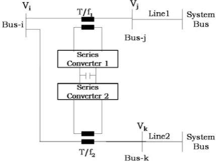
In its general form the interline power flow controller employs a number of dc-to-ac converters each providing series compensation for a different line. In other words, the IPFC comprises a number of static synchronous series compensators. The simplest IPFC consists of two back-to-back dc-to-ac converters, which are connected in series with two transmission lines through series coupling transformers and the dc terminals of the converters are connected together via a common dc link as shown in Fig.1. In addition to providing series reactive compensation, any converter can be controlled to supply real power to the common dc link from its own transmission line [16].
2.2. Power Injection Model of IPFC
A mathematical model of IPFC based on power injection is derived. This model is useful to study the impact of the IPFC on the power system network and can be incorporated in the power flow method. Usually, in the steady state analysis of power systems, the VSC may be represented as a synchronous voltage source injecting an almost sinusoidal voltage with controllable magnitude and angle. Based on this, the equivalent circuit of IPFC is shown in Fig.2.
The complex voltages at IPFC connected buses can be expressed as
(1)
The voltage magnitude at the series connected transformers having impedances can be expressed as
(2)
The power injection model is obtained by converting the series voltage sources to an equivalent current sources using Norton’s theorem and these sources are connected in parallel with the coupling transformers. The complex current entered into system can be expressed as
(3)
The equivalent power injected at the IPFC sending bus can be derived as
(4)
The respective real and reactive powers at ith bus can be expressed as
(5)
(6)
Similarly, the apparent power injected at IPFC receiving ends can be derived as
(7)
The respective real and reactive powers at jth and kth buses can be expressed as
(8)
(9)
Based on Eqns. (5), (6), (8), and (9), power injection model of IPFC can be seen as three power injections at buses i, j and k as shown in Fig.3.
The power balance equation that the IPFC should satisfy with respect to the AC system i.e. the active power exchange between the converters via the dc link is zero.
Where the superscript * denotes the conjugate of a complex number. 3. Load flow procedure with IPFC
The power balance equations and Jacobian matrix elements are modified due to IPFC. The modified power balance equations and Jacobian matrix elements are discussed in this section.
3.1. Power Balance Equations with IPFC
The IPFC power injection model can be incorporated into NR power flow algorithm by addition of power injections to the corresponding power mismatch equations. The modified power balance equations at IPFC connected buses can be expressed as
Where, the superscript ‘0’ denotes the power mismatch without IPFC respectively. 3.2. Jacobian Matrix Elements with IPFC
The relevant elements of Jacobian matrix are modified to consider the impact of IPFC model. The modified Jacobian matrix elements can be expressed as follows.
The modified diagonal and off-diagonal elements of with IPFC are
3.3. Overall computational procedure
The overall computational procedure of Newton-Raphson power flow method with IPFC can be described in the following steps.
Read bus data, line data and IPFC data.
Assume flat voltage profile and set iteration count K=0.
Compute active and reactive power mismatch from the scheduled and calculated powers. Determine Jacobian matrix using power flow equations.
Modify power mismatch and Jacobian matrix to incorporate IPFC model.
Solve the NR method equations to find the voltage angle and magnitude correction vector. Update the solution using correction vector.
Increase the iteration count, K=K+1.
Stop the process, when the maximum absolute mismatch is less than given tolerance and print the output. Otherwise, go to Step 3.
4. Optimal location
It is necessary to identify an optimal location to install IPFC in a given system. There are plenty of literatures, concentrated in identifying an optimal location based on severity index. This index is calculated based on the active/apparent power flows in transmission lines. Out of which, severity index and ranking methods is a popular method and having certain disadvantages. It cannot consider the stability of a transmission line into consideration. Hence in this paper, a new procedure is developed to identify an optimal location based line stability index (LSI). This index directly represents the stability of the system in terms of line loadings. The minimum and maximum limits for this index are ‘0’ (no-load condition) and ‘1’ (system collapse condition). This LSI index for a line connected between buses i and j can be represented as’
Where, X is the transmission line reactance, is the reactive power at receiving end of the transmission line, is the voltage magnitude at bus-I, are the voltage angles at the sending and receiving ends of the transmission line and is the impedance angle of the respective line. This index value is evaluated for each of the transmission line. The overall system index can be considered as the maximum value among all LSI values. To install IPFC, we require two transmission line connected at common bus. By the observation of all possible locations, in this paper, the following rules are formulated to decrease the computational effort and to increase the effectiveness of the device
IPFC should be connected between PQ buses only, where shunt compensators are not connected. IPFC should not place in a transformer connected lines.
List may be presented with each item marked by bullets and numbers. 5. Modified BAT algorithm
This algorithm is inspired from the echolocation of microbats [17-19]. It is metaheuristic population based optimization algorithm. Bats transmits some signals to the environment and then listen to its echo signals, this process is called as echolocation process. The velocity of the each of the population (N) is calculated using
Where, Gbest is the global best solution among all solutions. After calculating new velocities of each of the population is updated using
The frequency of signals transmitted by each of the bat is calculated as
Here, and are the maximum and minimum frequency values of each bat and is a random number between 0 and 1. After this modification of the positions of bats, there is one more modification in the positions using another fly, the new positions for each of the population can be calculated as
6. Results and Analysis
To study the effect of IPFC, IEEE-30 bus is considered on a computer with Intel core2Duo processor with 2GB RAM and installed with MATLAB software. The standard IEEE-30 bus system consists six generators, forty one transmission lines, two shunt compensating devices and four tap changing transformers is considered.
Initially the IPFC is installed in a location obtained using the procedure described in Section.5. Using this procedure and for this system, the possible installation locations to install IPFC are twenty one. The corresponding minimized line stability index values using BAT algorithm with IPFC in each of the locations are tabulated in Table.1. From this table, it is identified that, line stability index value is less in location-2 when compared to other locations. Hence, the series converters of IPFC are placed in the lines connected between buses 6, 7 and 28 with bus-6 as common to both converters. From this analysis, it is assumed that, the further analysis is performed by connecting IPFC in this location. The corresponding variation of LSI values in all locations is shown in Fig.4. The optimal settings of system and IPFC at minimized location are tabulated in Table.2.
Table.1 Line stability index values an all possible locations
Location No
IPFC sending
end
IPFC receiving
end-1
IPFC receiving
end-2
Table.2 Optimal settings at LSI minimized location with IPFC
S. No Control parameters Settings
1 Real power Gene rat io n ( M W) 148.1891 41.13655 34.43234 28.36953 20.56761 21.58646 2 Gene rat o r vol ta ges (p.u.) 1.080085 1.069585 0.999729 1.012289 1.019924 1.044848 3 Transformer tap
Fig.4 Variation of LSI values with IPFC
The further analysis is performed by varying the IPFC control parameters in the following five cases. Case-1: =0.02; =72; =0.1; =360
Case-2: =0.04; =144; =0.08; =288 Case-3: =0.06; =216; =0.06; =216 Case-4: =0.08; =288; =0.04; =144 Case-5: =0.1; =360; =0.02; =72
The voltage magnitudes and line apparent power flows for the following cases are tabulated in Tables 3 and 4 and the respective variations are shown in figures 5 and 6.
Table.3 Bus voltage magnitudes without and with IPFC
Bus No. Without
device Case-1 Case-2 Case-3 Case-4 Case-5
1 1.06 1.08 1.08 1.08 1.08 1.08
2 1.05 1.07 1.07 1.07 1.07 1.07
3 1.02 1.04 1.04 1.04 1.04 1.04
4 1.01 1.03 1.03 1.03 1.03 1.03
5 1.01 1 1 1 1 1
6 1.01 1.02 1.02 1.01 1.02 1.02
7 1 1 1.02 1.02 0.99 0.96
8 1.01 1.01 1.01 1.01 1.01 1.01
9 1.01 1.03 1.02 1.02 1.03 1.03
10 1.01 1.02 1.02 1.02 1.02 1.02
11 1.01 1.02 1.02 1.02 1.02 1.02
12 1.02 1.03 1.02 1.02 1.03 1.03
13 1.02 1.04 1.04 1.04 1.04 1.04
14 1.01 1.01 1.01 1.01 1.01 1.01
15 1 1.01 1.01 1.01 1.01 1.01
16 1.01 1.02 1.01 1.01 1.02 1.02
17 1.01 1.01 1.01 1.01 1.02 1.02
18 1 1 1 1 1 1
19 0.99 1 1 1 1 1
20 0.99 1 1 1 1.01 1.01
21 1 1.01 1.01 1.01 1.01 1.01
22 1 1.01 1.01 1.01 1.01 1.01
23 0.98 1 1 1.01 1.01 1.01
24 1 0.99 1 1.01 1.01 1.01
25 0.97 0.97 1 1.02 1.02 1.01
26 0.95 0.96 0.98 1 1 0.99
27 0.99 0.97 1 1.03 1.03 1.01
28 0.95 0.95 0.99 1.04 1.03 1.01
29 1 0.95 0.98 1.02 1.01 0.99
30 0.99 0.94 0.97 1 1 0.98
Table.4 Line apparent power flows without and with IPFC
Without
device Case-1 Case-2 Case-3 Case-4 Case-5
179.83 90.88 88.1 87.6 91.37 98.75
83.26 60.9 59.29 59.14 61.13 65.15
45.96 46.73 45.96 46.22 47.12 49.54
77.93 56.81 55.22 55.02 56.96 60.83
83.12 62.37 61.72 62.15 63.23 66.83
61.96 62.1 63.26 63.83 63.86 63.12
71.65 63.5 60.31 60.13 69.97 85.4
18.12 66.43 66.53 66.67 68.6 65.96
37.54 29.76 17.98 7.68 15.37 26.43
30.6 15.94 12.62 11.55 13.45 14.46
28.76 11.22 9.85 9.94 10.61 10.67
15.84 20.79 20.65 20.61 20.79 20.92
16.14 33.79 31.33 31.17 32.4 32.6
28.55 26.31 23.83 23.6 25.02 25.85
46.48 25.43 25.91 25.85 25.01 24.76
10.73 8.45 8.05 7.95 8.13 8.25
8.25 20.36 18.79 18.57 19.39 19.81
19.23 8.53 8.19 8.09 8.27 8.51
8.01 1.96 1.56 1.52 1.75 1.85
1.75 4.86 4.47 4.4 4.69 4.97
3.98 6.46 6.54 6.49 6.44 6.53
6.28 3.19 3.23 3.16 3.14 3.26
2.9 7.32 7.16 7.17 7.29 7.28
7.21 9.79 9.63 9.64 9.76 9.74
9.68 7.62 7.65 7.82 8.01 7.97
6.88 19.64 17.14 16.31 17.46 18.08
18.62 9.53 7.9 7.41 8.19 8.56
8.86 2.05 3.94 5.33 4.95 4.09
2.39 6.94 4.93 4.94 6.09 6.39
5.9 8.32 4.23 4.63 6.73 6.9
6.4 3.57 1.85 2.8 3.81 3.77
2.29 5.26 4.03 3.31 2.28 1.27
2.26 4.27 4.27 4.26 4.26 4.26
4.26 2.13 6.51 7.6 5.67 3.67
4.85 12.29 10.39 11.79 13.99 13.27
18.86 6.43 6.42 6.41 6.41 6.41
6.41 7.31 7.29 7.28 7.28 7.29
7.28 3.76 3.76 3.75 3.75 3.75
3.75 14.34 14.11 14.73 12.81 11.36
0.67 24.61 34.21 33.19 21.66 9.09
Fig.6 Variation of line apparent power flows without and with IPFC
The total active and reactive power flows without and with IPFC in the considered five cases is tabulated in Table.5 and the respective variation of active power losses is shown in Fig.7. From this, it is identified that, the maximum power losses are obtained without IPFC and minimum power losses are obtained in Case-3 with IPFC.
Table.5 Total power losses without and with IPFC
Without
device Case-1 Case-2 Case-3 Case-4 Case-5
P losses (MW) 17.64 12.74 11.71 11.54 12.79 15.41
Q losses (MVAr) 34.41 42.58 30.81 18.43 18.59 42.66
Fig.7 Variation of active power losses without and with IPFC
7. Conclusion
References
[1] L. Gyugyi, C. D. Schauder and K. K. Sen, “Static synchronous series compensator: a solid state approach to the series compensation of
transmission lines,” IEEE Trans. Power Del., Vol.12, No. 1, Jan. 1997, PP. 406–417.
[2] K. K. Sen, “SSSC-static synchronous series compensator: theory, modeling and applications,” IEEE Trans. Power Del., Vol.13, No. 1,
Jan. 1998, PP. 241–246.
[3] M.H.Haque and C.M.Yam, “A simple method of solving the controlled load flow problem of a power system in the presence of
UPFC,” Electric Power Syst. Research, Vol.65, 2003, PP. 55-62.
[4] Mehmet tumay, A.M.Vural and K.L.Lo, “The effect of unified power flow controller location in power systems,” Electrical Power and
Energy Syst., Vol. 26, 2004, PP. 561-569.
[5] Yankui Zhang, Yan Zhang and Chen Chen, “A novel power injection model of IPFC for power flow analysis inclusive of practical
constraints,” IEEE Trans. Power Syst., Vol.21, No.4, Nov.2006, PP.1550-1556.
[6] Jun Zhang and A.Yokoyama, “A comparison between the UPFC and the IPFC in optimal power flow control and power flow
regulation,” Proc.of IEEE Int.Conf., 2006, PP. 339-345.
[7] A.M.Vural and Mehmet tumay, “Mathematical modeling and analysis of a unified power flow controller: A comparison of two
approaches in power flow studies and effects of UPFC location,” Electrical Power and Energy Syst., Vol. 29, 2007, PP. 617-629.
[8] Ghadir Radman and Reshma S Raje , “Power flow model/calculation for power systems with multiple FACTS controllers,” Electric
Power Syst. Research, Vol.77, 2007, PP. 1521-1531.
[9] K. R. Padiyar and Nagesh Prabhu, “Analysis of SSR with three level twelve pulse VSC based interline power flow controller,” IEEE
Trans. Power Del., Vol.22, No. 3, Jul. 2007, PP. 1688–1695.
[10] Xia Jiang, X.Fang, J.H.Chow, A.A.Edris, E.Uzunovic, M.Parisi and L.Hopkins, “A novel approach for modeling voltage sourced
converter based FACTS controllers,” IEEE Trans. Power Del., Vol.23, No. 4, Oct.2008, PP. 2591–2598.
[11] R.Leon Vasquez Arnez and L.C.Zanetta, “A novel approach for modeling the steady state VSC based multiline FACTS controllers and
their operational constraints,” IEEE Trans. Power Del., Vol.23, No. 1, Jan.2008, PP. 457–464.
[12] S.Rajeswari, R.Gnanadass and P.Venkatesh, “Modelling of unified power flow controller for active power regulation,” Journal of
Electrical Engg., Vol. 90, Jun.2009, PP. 33-39.
[13] V.Azbe and R.Mihalic, “Energy function for an interline power flow controller,” Electric Power Syst. Research, Vol.79, 2009, PP.
945-952.
[14] Suman Bhowmick, Biswarup Das and Narendra Kumar, “An advanced IPFC model to reuse Newton power flow codes,” IEEE Trans.
Power Syst., Vol.24, No.2, May 2009, PP.525–532.
[15] Xinghao Fang, J.H.Chow, Xia Jiang, B.Fardanesh, E.Uzunovic, and A.A.Edris, “Sensitivity methods in the dispatch and siting of
FACTS controllers,” IEEE Trans. Power Syst., Vol.24, No. 2, May 2009, PP. 713–720.
[16] N.G.Hingorani and L.Gyugyi, “Understanding FACTS-concepts and technology of flexible AC transmission systems,” IEEE press,