https://doi.org/10.5194/esd-9-15-2018
© Author(s) 2018. This work is distributed under the Creative Commons Attribution 4.0 License.
Systematic Correlation Matrix Evaluation (SCoMaE)
– a bottom–up, science-led approach
to identifying indicators
Nadine Mengis1,a, David P. Keller2, and Andreas Oschlies2,3
1Geography, Planning, and Environment, Concordia University, Montréal, QC, Canada
2GEOMAR Helmholtz Centre for Ocean Research Kiel, Department
of Marine Biogeochemistry, 24105 Kiel, Germany
3Kiel University, 24098 Kiel, Germany
aformerly at: GEOMAR Helmholtz Centre for Ocean Research Kiel,
Department of Marine Biogeochemistry, 24105 Kiel, Germany
Correspondence:Nadine Mengis ([email protected])
Received: 1 August 2017 – Discussion started: 8 August 2017
Revised: 24 November 2017 – Accepted: 28 November 2017 – Published: 15 January 2018
Abstract. This study introduces the Systematic Correlation Matrix Evaluation (SCoMaE) method, a bottom–up
approach which combines expert judgment and statistical information to systematically select transparent, nonre-dundant indicators for a comprehensive assessment of the state of the Earth system. The methods consists of two basic steps: (1) the calculation of a correlation matrix among variables relevant for a given research question and (2) the systematic evaluation of the matrix, to identify clusters of variables with similar behavior and respective mutually independent indicators. Optional further analysis steps include (3) the interpretation of the identified clusters, enabling a learning effect from the selection of indicators, (4) testing the robustness of identified clus-ters with respect to changes in forcing or boundary conditions, (5) enabling a comparative assessment of varying scenarios by constructing and evaluating a common correlation matrix, and (6) the inclusion of expert judgment, for example, to prescribe indicators, to allow for considerations other than statistical consistency. The example
application of the SCoMaE method to Earth system model output forced by different CO2 emission
scenar-ios reveals the necessity of reevaluating indicators identified in a historical scenario simulation for an accurate assessment of an intermediate–high, as well as a business-as-usual, climate change scenario simulation. This necessity arises from changes in prevailing correlations in the Earth system under varying climate forcing. For a comparative assessment of the three climate change scenarios, we construct and evaluate a common correlation matrix, in which we identify robust correlations between variables across the three considered scenarios.
1 Introduction
An indicator is a quantitative value, measured or calculated, that describes relevant aspects of the state of a defined sys-tem. A useful indicator should fulfill certain characteristics that depend on the purpose of the indicator (Gallopín, 1996). Environmental indicators are developed based on quantita-tive measurements or statistics of environmental conditions in order to allow for a comparison of states of the envi-ronment across time or space (Ebert and Welsch, 2004).
fact that the indicators chosen should not provide redundant information.
For the assessment of ongoing climate change, models representing the physical and biogeochemical processes of the Earth system and known as Earth system models (ESMs) are one of the essential tools because the inertia of the cli-mate system to (carbon) perturbations requires projections of future climate states. Early climate models applied simple zero- to two-dimensional calculations to assess the effect of
atmospheric CO2on the climate by using global mean
sur-face air temperature (SAT) as an indicator (e.g., Arrhenius, 1896; Callendar, 1938; Sellers, 1969). This commonly used climate change indicator, SAT, fulfills all three abovemen-tioned characteristics. Several long-term temperature records as well as proxies for assessing SAT exist, which makes this indicator well measured (Statistical measurability). SAT is closely linked to other climate variables, e.g., evaporation, sea level rise, or biological productivity. Although SAT may not be the most relevant variable for society, using this in-dicator as a proxy for climate impacts is scientifically con-sistent (Seneviratne et al., 2016). Its political, economical, and ethical relevance evolved over time and is now evident in discussions concerning, e.g., global warming (Ott et al.,
2004) or the 2◦temperature increase target, which was
en-dorsed by the Conference of the Parties in 2015 (UNFCCC, 2015). Working group II of the Intergovernmental Panel on Climate Change (IPCC) (Houghton et al., 2001) used SAT as the main climate change indicator, due to its predominance in the existing literature and its large scientific consistency as such.
But as Earth system models and observational data sets continuously increase in complexity, there are more and more variables available that could potentially serve as indicators of the state of the climate system. Which ones should we select for a fully comprehensive assessment of changes in the climate system, ideally, without providing redundant in-formation? A common bottom–up approach for measuring complex systems is to start from a broad set of (Earth system) variables and consecutively select more appropriate ones de-pending on the research question (e.g., Pintér et al., 2005; Kopfmüller et al., 2012). For science-led climate change as-sessments reports, such as published by Working Group I of the IPCC, in addition to SAT, nowadays more indicators are selected to evaluate changes in different components of the Earth system, e.g., precipitation or often precipitation ex-tremes, Arctic summer sea ice, or the rate of ocean acidi-fication. Therefore, they are discussed in, e.g., the IPCC’s summary for policy makers of the recent assessment report of climate change (Stocker et al., 2013).
The selection of a limited number of indicators that sup-port scientific or political decision making is a major chal-lenge for experts, who in this case have to decide on the rel-ative importance of a variable in relation to others (Ramet-steiner et al., 2011). There exist no unambiguous rules for the selection process (Böhringer and Jochem, 2007). Any
in-dicator selection or metrics construction from Earth system variables implies a value and weighting decision and applies a weight of 0 to any disregarded variable. While the value judgment ideally requires the inclusion of potential end users or stakeholders, the weighting requires a well-informed and broad participation of scientific disciplines, i.e., expert judg-ment (Radermacher, 2005). However, selecting one indica-tor, while disregarding the other is a normative choice (Krel-lenberg et al., 2010), which can (unknowingly) be biased by, e.g., technical knowledge (Rametsteiner et al., 2011). Fur-thermore, Rametsteiner et al. (2011) point out that the ad hoc defined indicators should be subject to reevaluation over time.
In this study we want to introduce a bottom–up indicator selection method that uses statistical information about vari-ables in addition to expert judgement, thereby attempting to reduce bias in the selection process. Systematic Correlation Matrix Evaluation (SCoMaE) uses information on correla-tions between variables to identify “clusters” of variables that show similar behavior. We then systematically select scien-tifically consistent indicators to represent these clusters. The identified indicators are independent and do not provide re-dundant information. A set of independent indicators hence allows for a more comprehensive science-led assessment of the system under consideration than a set of correlated indi-cators. Furthermore, SCoMaE allows for a learning process by providing new information about correlations between the given variables and hence increases the system understand-ing.
To illustrate the SCoMaE method, we exemplarily select indicators to answer the following research question: “How are changes in the climate system influenced by the sensitiv-ity of the marine and terrestrial biological system to
tempera-ture and CO2?” This example application enables us to (1)
il-lustrate how a correlation matrix can be constructed given a specific research question, (2) identify a comprehensive in-dicator set, (3) show that an inin-dicator set derived from a cer-tain forcing scenario is not necessarily appropriate to assess a changed forcing scenario, (4) identify a common indicator set valid for multiple forcing scenarios, and finally (5) illus-trate how the method could be used in an iterative process in-cluding expert judgment or previous knowledge of the given system. These steps will serve as the guideline of this paper.
2 Defining the research question for the SCoMaE
example case
Before the SCoMaE method can be applied, it is crucial to identify and formulate the research question. For our ex-ample we chose to address the following research question: “How are changes in the climate system influenced by the sensitivity of the marine and terrestrial biological system to
temperature and CO2?” While for this question we chose to
intermediate-complexity Earth system model (see Sect. 2.1 and 2.3 for de-tails), it is possible to apply this method to other data sets to answer different questions. Here are a few examples of alter-native ways to define research questions and use the SCoMaE method to investigate them.
1. Our application is comparable with a multi-model en-semble where each of the perturbed parameters is a slightly different version of the default model. We could hence do the very same analysis as described in Sect. 3, with, e.g., the different models and scenar-ios simulated in the Coupled Model Intercomparsion Project 5 (CMIP5). The research question of how sim-ulated changes in the climate system are influenced by multi-model model variability under climate change could be answered by this setting.
2. To select indicators to answer the research question of which changes in the simulated Earth system are robust throughout state-of-the-art Earth system mod-els, we could again use the CMIP5 data sets. Here, one would probably want to calculate correlations be-tween time series of different variables. This would give information about similar frequencies of those vari-ables, which in turn suggests similar underlying pro-cesses. One could compare correlation matrices of one model during different forcing scenarios, as described in Sect. 3.3 and 3.4, or check the robustness of the cor-relations in one time period across models.
3. In that sense SCoMaE could also be applied to cal-culate correlations of observational time series. Since there is a higher level of noise within this data, it is possible to concentrate the research question on prede-fined timescales and filter the time series of the variables before applying the SCoMaE method. The indicators would accordingly be selected to answer the following underlying research question: “Which are the indepen-dent processes that I need to study for a comprehensive assessment of changes in the climate system of a given frequency band?”
Coming back to our example application of the SCoMaE method, we now want to briefly explain the model setup and simulations.
2.1 Model description
This paper illustrates the SCoMaE method for the example of model simulations performed with version 2.9 of the Univer-sity of Victoria Earth System Climate Model (UVic ESCM), an Earth system model of intermediate complexity (Eby et al., 2013). It includes schemes for ocean physics based on the Modular Ocean Model Version 2 (MOM2) (Pacanowski, 1995), ocean biogeochemistry (Keller et al., 2012), and a ter-restrial component including soil and vegetation dynamics
(Meissner et al., 2003). It is coupled to a thermodynamic sea ice model (Bitz et al., 2001) with elastic visco-plastic rhe-ology (Hunke and Dukowicz, 1997). The atmosphere is rep-resented by a two-dimensional atmospheric energy moisture balance model (Fanning and Weaver, 1996). All model
com-ponents have a common horizontal resolution of 3.6◦
lon-gitude and 1.8◦ latitude and the oceanic component has a
vertical resolution of 19 levels, with vertical thickness vary-ing from 50 m near the surface to 500 m in the deep ocean. Wind velocities used to calculate the advection of atmo-spheric heat and moisture as well as the air–sea-ice fluxes of surface momentum and heat and water fluxes, are prescribed as monthly climatological wind fields from NCAR/NCEP re-analysis data (Eby et al., 2013). Wind anomalies, which are determined from surface pressure anomalies with respect to preindustrial surface air temperature, are added to the pre-scribed wind fields.
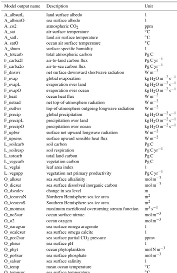
A list of the globally aggregated output variables is given in Table A1.
2.2 Spin-up and scenario forcing
For the default model simulation, the UVic ESCM was spun-up with preindustrial (year 1765) seasonal forcing for over 10 000 years. All simulations were integrated from 850 un-til 2005 using historical fossil-fuel emissions and land-use changes, as well as radiative forcing from solar variability and volcanic activity following Eby et al. (2013). Following Keller et al. (2014), continental ice sheets were held constant to facilitate the experimental setting and analyses. Warming from black carbon, indirect ozone effects, and cooling from indirect sulfate aerosol effects were not included. From 2005 onward until 2100 the Representative Concentration Pathway (RCP) 4.5 and 8.5 scenarios from Meinshausen et al. (2011)
were implemented as an intermediate and high-CO2
emis-sions driven scenario, respectively.
For the sensitivity analysis performed with the UVic ESCM, different model input parameters and parameteriza-tions were perturbed, and for some of them it was necessary to do a new model spin-up to reach steady-state conditions again; apart from this the forcing was the same for all simu-lations.
2.3 Parameter perturbations
In the following sections, the single-parameter perturbation experiments, which are used in the example and shown in Fig. 1, are explained in detail. We chose these parameters to explore the sensitivity of the UVic ESCM to uncertainties in terrestrial and marine biological productivity with respect
to temperature and CO2, since these processes will
2000 2020 2040 2060 2080 2100 13 14 15 16 17 18 [
o C]
Surface Air Temperature
2000 2020 2040 2060 2080 2100 10 12 14 16 18 20 [Sv]
Maximum Ocean Overturning
2000 2020 2040 2060 2080 21004 6 8 10 12 [Million km ] 2
NH sea ice area
2000 2020 2040 2060 2080 2100 650 700 750 800 850 900 950 [mm yr − 1]
Precipitation over Land
Subtract
Subtract
Calculate
correlation
F_precipLF_evapLF_upsensF_carba2oO_phytA_albsurLO_no3surO_salsurL_veglaiF_precipF_evapO_o2
O_po4surO_alksurL_vegcarbL_vegnppO_totcarbF_uplwrF_outlwrF_precipOF_heatF_netradL_soilrespO_dsealevO_ocalcsurO_tempO_oaragsurF_carba2lL_soilcarbL_totcarbO_phsur O_iceareaNA_albsurOO_iceareaSO_motmaxF_dnswrO_dicsurA_totcarbO_pco2surA_co2F_evapOA_shum
O_tempsur A_satLA_satOA_sat
Correlations of changes in the SRM run
F_ precipLF_ evapL F_ upsensO_ phyt F_ carba2oA_ albsurL O_ no3surO_ salsur L_ veglai F_ precipF_ evap O_ o2 O_ po4surO_ alksur L_ vegcarbL_ vegnpp O_ totcarbF_ uplwr F_ outlwr F_ precipOF_ heat F_ netrad L_ soilresp O_ dsealevO_ temp O_ ocalcsur O_ oaragsurF_ carba2l L_ soilcarbL_ totcarb O_ phsur O_ iceareaNA_ albsurO O_ iceareaSO_ motmax F_ dnswr O_ dicsur A_ totcarbA_ co2 O_ pco2surF_ evapO A_ shum O_ tempsurA_ satL A_ satOA_ sat −1 −0.8 −0.6 −0.4 −0.2 0 0.2 0.4 0.6 0.8 1 Correlation matrix
NH se
a ice
area
SAT
Put information into matrix Surface air temperature (SAT)
20502100 −50 0 50 100 150 Radiatio RCP8.5 RCP8.5 Kv low Kv high No marine T sens No terr. T sens. Veg. q10 low Veg. q10 high Soil q10 low Soil q10 high CO2 fert zero CO2 fert low CO2 fert high transp. CO2 sens zero transp. CO2 sens low transp. CO2 sens high CN CO2 sens
20502100 −50 0 50 100 150 Radiatio RCP8.5 rcp85 Kv low Kv high no marine T sens no terr. T sens veg q10 low veg q10 high soil q10 low soil q10 high CO fert. zero2 CO fert. low2 CO fert. high2 Transp. CO sens. zero2 Transp. CO sens. low2 Transp. CO sens. high2 CN CO sens.2 Correlation = -0.955
.
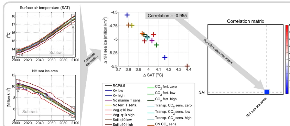
Figure 1.Illustration of the correlation matrix construction for the example case study, and the model output variables surface air
tempera-ture (SAT) and Northern Hemisphere (NH) sea ice area. In the first step, temporal differences of the simulations are calculated between 2005– 2015 and 2090–2100. Second, changes in the variables induced by the parameter perturbations are correlated. Last, this correlation informa-tion is used as one of many entries in the correlainforma-tion matrix.
Table 1.List of perturbed model input parameters.
Abbreviation Short explanation of parameter perturbation
Kv low lower bound of vertical ocean diffusivity
Kv high higher bound of vertical ocean diffusivity
No marineT sens. no marine biological sensitivity to temperature
No terr.T sens. no terrestrial vegetation sensitivity to temperature
Veg. q10 low lower bound of the vegetationQ10sensitivity
Veg. q10 high higher bound of the vegetationQ10sensitivity
Soil q10 low lower bound of the soilQ10sensitivity
Soil q10 high higher bound of the soilQ10sensitivity
CO2fert. zero no CO2fertilization effect
CO2fert. low lower bound of CO2fertilization effect
CO2fert. high higher bound of CO2fertilization effect
Transp. CO2sens. zero no CO2sensitivity of transpiration
Transp. CO2sens. low lower bound of CO2sensitivity of transpiration Transp. CO2sens. high higher bound of CO2sensitivity of transpiration
CN CO2sens. stoichiometric changes in response to changing ocean carbonate chemistry
based on their agreement with the time series of the histori-cal global mean air temperature (Fig. S5). See Table 1 for a quick overview of the simulations.
2.3.1 Vertical ocean diffusivity
Small-scale physical mixing (vertical diffusivity or diapyc-nal mixing) in the ocean is parameterized in all global mod-els because of their resolution. Thus, this important process, which plays a key role in determining ocean circulation and biogeochemical cycles as well as ocean to atmosphere heat
2.3.2 Lower bounds of biological temperature sensitivity
Although biological processes are known to be sensitive to temperature, there is a significant amount of uncertainty in how biology will respond to warming caused by climate change (Friedlingstein et al., 2006; Taucher and Oschlies, 2011). Furthermore, there are many different ways to model the effects of temperature on biology, and it is not know which is best for Earth system model applications. To inves-tigate the lower bounds of the sensitivity of biological pro-cesses to direct temperature effects, we conduct simulations where direct temperature effects on biology are not included. In order to ensure that global biogeochemical fluxes are as close to present-day ones as possible, flux-weighted global averages for temperature-dependent rates were set for all temperature-dependent functions (see Taucher and Oschlies, 2011 for details). This approach was applied separately to marine and terrestrial ecosystems:
a. No marine biological sensitivity to temperature: the re-sults of this analysis can be used to estimate a lower boundary for how marine plankton and how their ef-fect on biogeochemical cycles will respond directly to
global warming (no marineT sens.). For this sensitivity
analysis, the model was spun-up with the corresponding setting for 10 000 years until a new equilibrium climate state was reached.
b. No terrestrial vegetation sensitivity to temperature: the results of this analysis can be used to estimate a lower boundary for how terrestrial vegetation and its effect on the carbon cycle will respond directly to global
warm-ing (no terr. T sens.). For this sensitivity analysis, the
model was spun-up with the corresponding setting for 10 000 years until a new equilibrium climate state was reached.
2.3.3 Vegetation and soil sensitivity to temperature
To further investigate the sensitivity of terrestrial biology to
temperature, we varied the vegetation and soilQ10 values,
which are observationally derived coefficients that are used to model the biological system rate of change in response to a
10◦C temperature increase. Low and highQ10values of 1.5
and 3.0 (model default is 2.0), which are within the range of observational estimates (Lloyd and Taylor, 1994), were set to investigate how different terrestrial biological sensitivities to temperature affect the model results (veg. q10 low/high and soil q10 low/high). For this sensitivity analysis, the model was spun-up with the corresponding setting for 10 000 years until a new equilibrium climate state was reached.
2.3.4 CO2fertilization of vegetation
Increasing atmospheric CO2 is thought to stimulate
terres-trial carbon uptake through the process of CO2fertilization
(Matthews, 2007; Keenan et al., 2013). This negative
car-bon cycle feedback results in reduced atmospheric CO2
con-centrations and has likely accounted for a substantial por-tion of the historical terrestrial carbon sink (Friedlingstein
et al., 2006). However, the future strength of CO2
fertiliza-tion in response to continued carbon emissions is highly un-certain. In order to test the impact of this uncertainty for fu-ture climate change simulations, we followed the approach of
Matthews (2007) by scaling the CO2sensitivity of the
terres-trial photosynthesis model. We performed a simulation with
no CO2fertilization effect (CO2fert. zero), as well as two
simulations where we varied the strength of the CO2
fertil-ization effect by increasing and decreasing it by 50 % (CO2
fert. high/low) relative to the default model. No additional
model spin-up was needed since the simulated CO2
fertiliza-tion effect only happens when the atmospheric CO2
concen-tration begins to increase, e.g., from the preindustrial period onward.
2.3.5 CO2sensitivity of transpiration
Transpiration by plants is highly sensitive to increases in
at-mospheric CO2, since plants tend to open their stomata less
often in higher-CO2environments in order to reduce water
loss to the atmosphere. The strength of this effect and its im-pacts on climate are highly uncertain and have been studied both through observations and models (Keenan et al., 2013; Van Der Sleen et al., 2014; Mengis et al., 2015). To test how strongly this affects simulations of future climate, the amount of transpiration for all plant functional types was scaled after
Mengis et al. (2015). In this approach the CO2fertilization
effect is not changed. Three simulations were performed: for the first simulation, transpiration did not change relative to
the preindustrial level (transp. CO2sens. zero); for the other
two simulations, the scaled transpiration was increased and decreased by 50 % of the amount that the model would
sim-ulate with the default setting (transp. CO2 sens. high/low)
as CO2changes. No additional model spin-up was needed,
since the effect of changing CO2 on transpiration only
be-comes evident when the atmospheric CO2concentration
be-gins to increase, e.g., from the preindustrial period onward.
2.3.6 Stoichiometric changes in response to changing ocean carbonate chemistry
Mesocosm studies that artificially increase the amount of
CO2 in seawater (e.g., climate change experiments) have
suggested that the C : N content of marine plankton may be sensitive to changes in carbonate chemistry. The mesocosm
study of Riebesell et al. (2007) suggested that as CO2
mesocosm-derived relationship between the atmospheric CO2 concen-tration and the C : N content of plankton as in Oschlies et al.
(2008) (CN CO2 sens.). No additional model spin-up was
needed, since the effect of changing CO2on plankton
stoi-chiometry only becomes evident when the atmospheric CO2
concentration begins to increase, e.g., from the preindustrial period onward.
3 The Systematic Correlation Matrix
Evaluation (SCoMaE) method
3.1 Step 1: calculate the correlation matrix
Throughout this study, a variable is defined as a model out-put or observational time series, whereas we refer to it as an indicator if a variable was selected to represent a certain as-pect of the considered system. To obtain a comprehensive, nonredundant set of indicators to describe a given system, the first step is to construct a correlation matrix, i.e., a ma-trix including the correlation information of all the relevant Earth system variables to each other. The construction of the correlation matrix strongly depends on the research ques-tion and needs to be adjusted accordingly. The selecques-tion of which variables are the relevant variables for the given re-search question and hence should be included in the matrix, as well as the choice of how the correlations should be cal-culated is very important for the outcome of the study. In the same way, it is important to consider a reasonable signal-to-noise ratio within the data set chosen. Correlations could for example be calculated between time series of variables or their derivatives, absolute temporal changes, or spatial pat-terns. Alternatively, output from ensemble simulations could be used to calculate correlations between changes in vari-ables due to the different ensemble members. The matrix is then evaluated based on the significance information of these correlations (see Step 2). Note that for this preselection of the possibly relevant variables to answer the given question, as well as for the construction of the correlation information in the matrix, a certain level of expert judgement is needed.
To illustrate the construction of the matrix based on our example simulations, we show how the correlation between changes in global mean “surface air temperature” (A_sat) and “Northern Hemisphere sea ice area” (O_iceareaN) in the Representative Concentration Pathway (RCP) 8.5 emission scenario (Meinshausen et al., 2011) due to the parameter per-turbations translates to the corresponding correlation matrix entry (Fig. 1). In our example we want to study the correla-tions between changes in model output variables, induced by varying poorly constrained model input parameters concern-ing the carbon cycle. In the followconcern-ing we will refer to these as “correlation of variable changes”.
Assuming that the signal of interest is of a similar kind as the state differences between the start and the end of a climate change simulation, we start by calculating the temporal dif-ferences between 2005–2015 and 2090–2100 from a number
of parameter perturbation simulations that serve as our en-semble in this example (see Sect. 2.3 for explanations of the parameter perturbations). This enables us to learn whether the different output variables show a similar behavior for the respective parameter perturbation. Then the Pearson corre-lation coefficients between these changes are calculated and tested by performing a two-sided test at a 5 % significance
level, withN=16, the number of perturbed parameter
sim-ulations, and accordinglytcrit=2.145.
In our example, there is a negative correlation of variable changes evident between “surface air temperature” (A_sat) and “Northern Hemisphere sea ice area” (O_iceareaN). This illustrates that these model output variables show consis-tent opposite reactions towards the parameter perturbations, i.e., if the perturbation causes surface air temperatures to increase, it also causes northern hemispheric sea ice to de-crease. This information is then written into the correlation matrix. By studying the constructed correlation matrix and studying single correlations of changes between model out-put variables, we can learn about basic processes within the simulated climate system and test whether these agree with our expectations. To simplify the visual analysis of our ex-ample we sorted the variables in the matrices according to their strength in correlation of variable changes relative to changes in the commonly used climate change indicator, i.e., “surface air temperature” (A_sat) in the historical scenario.
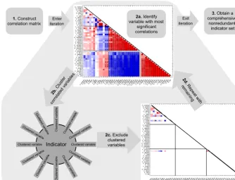
3.2 Step 2: cluster identification and indicator selection
To obtain a set of indicators for the assessment of changes in the system under consideration, we systematically evaluate the previously constructed correlation matrix (see Fig. 2 for an illustration of this procedure). To obtain a comprehensive, nonredundant indicator set, we follow these steps: (1) the first indicator is the variable with the highest number of signifi-cant correlations with other variables; (2) all variables with a significant correlation are clustered under this indicator; (3) these clustered variables are then excluded from the selec-tion of the next indicator; (4) the next indicator is again the variable with the highest number of significant correlations with all the remaining variables; (5) this indicator selection procedure is repeated until all variables are clustered and are represented by an indicator. If a variable is not significantly correlated to any of the remaining variables, this variable is considered to be a single indicator. These single indicators are needed for a fully comprehensive assessment, since they show different behavior from all previously selected indica-tors and hence provide additional information.
1. Construct correlation matrix
Exit
iteration
3. Obtain a
comprehensive,
nonredundant indicator set
2a. Identify
variable with most significant correlations
Enter
iteration
2d.
Re pe
at w
ith re ma ining 2b. Clu ster corre late
d va
riabl
es
2c. Exclude
clustered
variables Indicator Clustere d va riable Cl uste re d v ariab le Clus tere d va
riabl e Cl us te re d va ria bl e Cluste red va
riable Clustered variable Clustere d va riable Clustered variable Cl uste re d v ariab le Cluste red va
riable Cl us te re d va ria bl e Clus tere
d va riabl
e
Figure 2.Illustration of the indicator selection process using the example of the correlation matrix for the historical scenario (see Fig. 3
for a more detailed display of the correlation matrix). The correlation matrix, was constructed as explained in Fig. 1 but for the temporal differences between 1850–1860 and 1995–2005. See Sect. 3.2 for a detailed step-by-step description of the evaluation process. Prefixes A, O, L, and F stand for atmosphere, ocean, land, and fluxes, respectively; for a detailed description of the model output variables, see Table A1.
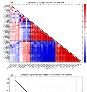
the respective column of F_precipO (17th from the right) in the correlation matrix, we can see that changes in this model output variable are significantly correlated to changes in all variables that are also significantly correlated to changes in “surface air temperature” (A_sat; first from the bottom), with the exception of “mean ocean temperature” (O_temp, 16th from the bottom) but in addition also link changes in global and terrestrial precipitation and evapotranspiration (F_precip, F_precipL and F_evap, F_evapL, respectively; 35th and 37th from the bottom) as well as changes in “surface net upward longwave radiation” (F_uplwr, 40th from the bot-tom). The changes in these variables due to parameter pertur-bations are not significantly correlated to changes in “surface air temperature” (A_sat). Hence, based on purely statistical considerations, using “precipitation over ocean” (F_precipO) as an indicator for the research question in the historical pe-riod would be preferable to global mean “surface air temper-ature” (A_sat), the main ad hoc indicator of historical climate change, since it potentially holds more information.
“Surface albedo on land” (A_albsurL) is identified as the second indicator. After excluding all variables correlated to changes in “precipitation over ocean” (F_precipO), its changes due to the parameter perturbations are significantly correlated to changes in “net surface downward shortwave radiation” (F_dnswr), “ocean oxygen” (O_o2), and “sea surface salinity” (O_salsur). The third indicator is “ocean
surface alkalinity” (O_alksur), which shows the same re-sponse to the parameter perturbations as “ocean surface phosphate concentrations” (O_po4sur). When excluding all variables that are clustered under one of the three abovemen-tioned indicators, three variables remain unclustered: “mean ocean temperature” (O_temp), “maximum meridional over-turning” (O_motmax), and “ocean phytoplankton” (O_phyt). These variables are hence single indicators, which are needed for a comprehensive assessment of the system under consid-eration (Fig. 3b).
See Sect. 1 and Figs. S1 and S2 in the Supplement for the results of these analyses for the intermediate–high (RCP4.5) and the business-as-usual (RCP8.5) scenarios, respectively.
3.3 Step 3 (optional): comparison of indicators for the different forcing scenarios
In order to learn how well the previously identified indicators for one scenario explain a different scenario with changed forcing, we prescribe the use of the previously identified in-dicator set. The SCoMaE accordingly first uses these tors and then analyses whether and which additional indica-tors are needed for a fully comprehensive assessment of the new scenario.
Figure 3.(a)Correlation matrix for the historical scenario. The correlations are calculated between changes in the 46 model output vari-ables for temporal differences between 1850–1860 and 1995–2005 from the results of the perturbed parameter simulations (as in Fig. 1). Correlations significant at a 5 % significance level are marked with crosses. The order of the variables was determined based on their cor-relation strength to “surface air temperature” (A_sat) in the historical scenario. Prefixes A, O, L, and F stand for atmosphere, ocean, land, and fluxes, respectively; for a detailed description of the model output variables, see Table A1.(b)Indicators as identified from the SCo-MaE analysis of the correlation matrix above as illustrated in Fig. 2, ranked by the amount of significant correlations. The indicators are as follows: “precipitation over ocean” (F_precipO), “land surface albedo” (A_albsurL), “ocean surface alkalinity” (O_alksur), “mean ocean temperature” (O_temp), “ocean phytoplankton” (O_phyt), and “ocean overturning” (O_motmax).
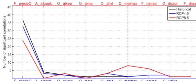
high (RCP4.5) and the business-as-usual (RCP8.5) emission scenarios (Fig. 4). The results show that if we were to only utilize the indicators from the historical scenario for the as-sessment of the two RCP scenarios, we would not be able to assess all changes in the climate system as represented by our model: for the RCP4.5 scenario, we would obtain ad-ditional information by considering the variables “net top-of-atmosphere radiation” (F_netrad) and “ocean surface heat flux” (F_heat), which are clustered together, and “net upward longwave radiation” (F_uplwr) and “ocean surface salin-ity” (O_salsur), which form another indicator cluster (Fig. 4). Note that Earth system variables clustered under the prescribed indicators differ among the different
F_ precipO A_ albsurL O_ alksur O_ temp O_ phyt O_ motmax F_ netrad F_ uplwr
5 10 15 20 25 30 35 40 45
Number of significant correlations
F_ precipO A_ albsurL O_ alksur O_ temp O_ phyt O_ motmax F_ netrad O_ dicsur F_ dnswr
Historical RCP4.5 RCP8.5
Figure 4.Indicators identified from the analysis of the RCP4.5 (blue) and RCP8.5 (red) correlation matrices with the precondition to use the
historical indicators first. The indicators are as follows: “precipitation over ocean” (F_precipO), “land surface albedo” (A_albsurL), “ocean surface alkalinity” (O_alksur), “mean ocean temperature” (O_temp), “ocean phytoplankton” (O_phyt), “ocean overturning” (O_motmax), “net radiation at the top of the atmosphere” (F_netrad), “ocean surface dissolved inorganic carbon” (O_dicsur), and “downward shortwave radiation” (F_dnswr).
The differences between the correlation matrices for the RCP8.5 scenario compared to the historical scenario are even larger (compare Figs. 3 and S2). For the RCP8.5 scenario, 8 out of 46 considered variables would not be included if we applied the indicators identified for the historical scenario. Instead we need three additional indicators for the assess-ment of the system under consideration, namely “net top-of-atmosphere radiation” (F_netrad), “ocean surface dissolved inorganic carbon” (O_dicsur), and “net surface downward shortwave radiation” (F_dnswr) (Fig. 4). Note that six of the eight remaining variables that were initially included in the first indicator cluster for the historical scenario, namely “precipitation over ocean” (F_precipO), are no longer signif-icantly correlated to it for the RCP8.5 scenario.
These differences in the correlation matrices for the dif-ferent forcing scenarios indicate changes in prevailing cor-relations between Earth system variables with the imposed climate forcing. This illustrates that a reevaluation of the in-dicators chosen may be needed for a comprehensive assess-ment of different climate strategies yielding different climate states.
3.4 Step 4 (optional): evaluation of a common correlation matrix
To advance this analysis such that changes in correlation ma-trices from different forcing scenarios can be taken into ac-count, it is possible to create a correlation matrix representing only those correlations that are significant in all forcing sce-narios; this is defined as a common correlation matrix. Ap-plying the SCoMaE method to such a common correlation matrix identifies an indicator set that can be used to assess and also compare multiple scenarios and which hence differs from the previously identified sets for the individual correla-tion matrices.
To obtain a common indicator set for the three example forcing scenarios (historical, RCP4.5, and RCP8.5), we con-struct a correlation matrix in which only correlations of vari-able changes that are significant in all these scenarios are considered (Fig. 5). Furthermore the color shading indicates in which of the scenarios the correlations between variable changes were found to be significant.
A first visual evaluation of the common correlation matrix shows more reddish than bluish shading, which indicates that the correlation patterns for the historical and RCP4.5 scenar-ios are more similar than for the historical and RCP8.5 sce-narios (Fig. 5). This means that for a lower future emission scenario, the indicators from the historical scenario are more suitable than for a higher future emission scenario. This is true with the exception of the terrestrial and oceanic car-bon fluxes (F_carba2l and F_carba2o, respectively). These two fluxes are perturbed by the land-use scheme imple-mented in the RCP4.5 scenario, since this scenario includes a high amount of afforestation and reforestation. Furthermore, greenish shading shows correlations of variable changes that are significant only in the RCP scenarios, indicating that those correlations of variable changes depend on the
increas-ing anthropogenic (mainly CO2) forcing, included only in
these scenarios.
The first indicator obtained from the common SCoMaE
analysis is “atmospheric CO2” (A_co2), which was also
found to be the first indicator in the RCP8.5 scenario (Figs. S7 and S8). Its changes are significantly correlated to changes in 27 other output variables in all three scenarios. This indicates that these correlations of variable changes are
robust throughout the different strength of CO2forcing in the
three scenarios. The fact that “atmospheric CO2” (A_co2)
Figure 5. (a)Correlation matrix for all three scenarios, merging the significance information from all three scenarios. Colors indicate in which scenario the changes in variables due to parameter perturbations showed a significant correlation; see color bar for an explana-tion. The crosses mark combinations of variables where the correlation of variable changes is significant at a 5 % significance level in all three scenarios. For details on the model output variables under consideration, see Table A1.(b)Indicators as identified from the anal-ysis based on the correlation matrix above against the number of significant correlations (blue) and with the condition that “surface air temperature” (A_sat) is prescribed as the first indicator (red). The indicators are as follows: “atmospheric carbon content” (A_co2), “precip-itation over land” (F_precipL), “atmosphere-to-ocean carbon flux” (F_carba2o), “net top-of-atmosphere radiation” (F_netrad), “net surface downward shortwave radiation” (F_dnswr), “atmosphere-to-land carbon flux” (F_carba2l), “ocean surface nitrate” (O_no3sur), “top-of-atmosphere outgoing longwave radiation” (F_outlwr), “ocean oxygen” (O_o2), “ocean surface alkalinity” (O_alksur), “ocean phytoplank-ton” (O_phyt), “ocean surface salinity” (O_salsur), “sea surface phosphate” (O_po4sur), “ocean overturning” (O_motmax), “precipitation over ocean” (F_precipO), “ocean carbon” (O_totcarb), and “surface net upward longwave radiation” (F_uplwr).
system variables with regard to the parameter perturbations, such as changes in temperatures, carbon fluxes, and moisture fluxes over the ocean. This can possibly be explained by the fact that the changes in these variables are sensitive to the
imposed CO2forcing, which in turn is reflected in the
atmo-spheric carbon concentration.
The second indicator is “precipitation over
land” (F_precipL), which is clustered with “terrestrial evapotranspiration” (F_evapL) and “net upward longwave radiation” (F_uplwr) (Fig. S6). This cluster accordingly represents changes in terrestrial moisture fluxes and the
flux” (F_carba2o) and “soil respiration” (L_soilresp); “net top-of-atmosphere radiation” (F_netrad) and the “ocean surface heat flux” (F_heat); and “net surface downward shortwave radiation” (F_dnswr) and the “land surface albedo” (A_albsurL).
The remaining single indicators are “air-to-land carbon flux” (F_carba2l), “ocean surface nitrate” (O_no3sur), “top-of-atmosphere outgoing longwave radiation” (F_outlwr),
“ocean oxygen” (O_o2), “ocean surface
alkalin-ity” (O_alksur), “ocean phytoplankton” (O_phyt), “sea
surface salinity” (O_salsur), “ocean surface
phos-phate” (O_po4sur), and “maximum ocean meridional overturning” (O_motmax).
3.5 Step 5 (optional): including expert judgment
If stakeholders or experts were to inform the indicator selec-tion process, it would be possible to prescribe indicators and then use the SCoMaE analysis to identify additional uncor-related variables that are needed to obtain a comprehensive assessment of the system. Also, instead of using global mean time series, one could look at time series of regions or al-ready processed variables, such as heat stress or cumulative emissions. This approach in combination with the SCoMaE analysis enables us to learn about variables which have pre-viously been disregarded but potentially provide new infor-mation about the system or to learn which of the indicators previously considered actually provide redundant informa-tion.
How would the common indicator set from our example change if we were to include the condition that surface air temperature should be the first indicator, instead of
atmo-spheric CO2?
Prescribing “surface air temperature” (A_sat) as the first indicator for the common correlation matrix leads to the re-placement of “precipitation over land” (F_precipL) by “pre-cipitation over ocean” (F_precipO) as the second indicator (Fig. 5b); its change with the parameter perturbations is cor-related with 12 variables that are clustered under this indi-cator. Almost all of these variables were initially clustered
under “atmospheric CO2” (A_co2) but are not significantly
correlated to changes in “surface air temperature” (A_sat). These variables mainly describe global and oceanic mois-ture fluxes, as well as carbon fluxes or reservoirs on land: “precipitation over the ocean” (F_precipO), “global evapo-ration” (F_evap), “global precipitation” (F_precip), “vege-tation net primary productivity” (L_vegnpp), “leaf area in-dex” (L_veglai), “vegetation carbon” (L_vegcarb), and the “surface upward sensible heat flux” (F_upsens). The only ex-ception to this behavior is “total ocean carbon” (O_totcarb), which in turn becomes a single indicator. In addition the sec-ond indicator, “precipitation over the ocean” (F_precipO), now incorporates the previously identified clusters of the second and third indicators, namely the clusters of “pre-cipitation over land” (F_precipL) and the “air-to-sea
car-bon flux” (F_carba2o). Only “net upward longwave radia-tion” (F_uplwr), which was also clustered under “precipita-tion over land” (F_precipL) becomes a single indicator, re-maining unclustered when “surface air temperature” (A_sat) is prescribed as the primary indicator. In turn, “air-to-land carbon flux” (F_carba2l), which was a single indicator in the default SCoMaE analysis, is now clustered under “surface air temperature” (A_sat).
The third and fourth indicators are “net top-of-atmosphere radiation” (F_netrad) and “net surface downward shortwave radiation” (F_dnswr), which were found with the same un-derlying clusters in the default analysis (compare Figs. S8 and S9). Finally, eight of the nine previously identified sin-gle indicators remain unclustered and hence are still sinsin-gle indicators.
Although the total number of indicators has not changed, the identified clusters and their meaning differ: in the default analysis, the first indicator represented changes in tempera-tures, carbon fluxes, and global and oceanic moisture fluxes. If “surface air temperature” (A_sat) is prescribed, the global and oceanic moisture fluxes are moved to the second cluster, which in addition incorporates some Earth system variables from the previously identified second and third indicators. This is one example showing how the SCoMaE method al-lows for the inclusion of expert judgment or preconditions, is able to account for changes in correlation patterns, and allows one to determine which indicators are needed for a comprehensive and nonredundant assessment. (For more dis-cussions, see Sect. 2 and Fig. S3 in the Supplement.)
4 Discussion
4.1 Discussion of the results from the example 4.1.1 What were we able to learn from the example?
As illustrated above, the SCoMaE method statistically eval-uates the correlations between changes in model output vari-ables and uses this information to cluster varivari-ables, while selecting a representative indicator for each cluster. The ex-ample analyses of the individual scenarios illustrates the de-pendence of the indicator selection on the imposed forcing scenario. These results demonstrate that for our model, it is insufficient to apply the historical indicator set to the
fu-ture scenarios with either higher CO2forcing such as in the
RCP8.5 scenario or more limited CO2forcing and reduced
anthropogenic land use such as in the RCP4.5 scenario. Al-though our analysis is too limited to conclusively determine a best set of climate change indicators in a purely scientific bottom–up approach, our results do suggest that a compre-hensive assessment of future climatic states needs a reevalu-ation of the ad hoc indicators chosen, due to changes in pre-vailing climate responses.
correlation matrix to identify indicators that can be used for the assessment of all three scenarios. For the clusters of ables of the common indicator set, the correlations of vari-able changes remain significant even under different atmo-spheric carbon or land-use forcing.
However, one should always ask whether the identified clusters and indicators are scientifically meaningful. For the common correlation matrix (as well as the RCP8.5 scenario),
the first indicator, “atmospheric CO2” (A_co2), groups
to-gether variables describing changes in carbon fluxes, tem-peratures, and moisture fluxes over the ocean. This is scien-tifically meaningful, since changes in carbon fluxes will af-fect the atmospheric carbon content and hence atmospheric temperatures, both over land and ocean. These temperature changes in turn have an effect on the moisture fluxes over the ocean, such as the evaporation over ocean, which is phys-ically driven by temperature changes. These categories are hence physically linked, and it is to be expected that they are correlated irrespective of the forcing scenario chosen.
The second indicator, “precipitation over
land” (F_precipL), represents the variability of mois-ture fluxes on land and the associated cooling effect. The fact that these processes are clustered under an indicator that is distinct from global and oceanic moisture fluxes indicates different underlying processes for these moisture fluxes, namely the influence of biological transpiration. This process is directly affected by the parameter perturbations
concerning the sensitivity of transpiration to CO2 (Mengis
et al., 2015) and the CO2 fertilization effect (Matthews,
2007). Given the parameter sensitivities of the model considered, the distinction between terrestrial and marine moisture fluxes is scientifically meaningful.
Another identified cluster is “net top-of-atmosphere ra-diation” (F_netrad) and “ocean surface heat flux” (F_heat), which are directly linked in the model. Furthermore “net sur-face downward shortwave radiation” (F_dnswr) and “land surface albedo” (A_albsurL) are clustered, since changes in vegetation on land induced by the parameter perturbations influence both the surface albedo on land and the incoming shortwave radiation at the surface.
The “air-to-sea carbon flux” (F_carba2o) and “soil respi-ration” (L_soilresp) are clustered together for all three sce-narios but show a negative correlation of variable changes in the historical scenario and positive correlations of variable changes in the two RCP scenarios, indicating a dependency on the atmospheric carbon concentrations. The predominant parameterization for those correlations of variable changes is
one that affects the CO2fertilization (Fig. S7). Since this is
not an intuitive connection, we will briefly discuss this
corre-lation in more detail: the strength of the CO2fertilization
de-termines the increase in plant net primary production (NPP)
to increasing atmospheric CO2concentrations. For the
his-torical scenario, in the case when the CO2 fertilization
pa-rameterization is increased, soil respiration increases due to an increase in vegetation and hence the soil carbon pool. In
the same case, the air-to-sea carbon flux slightly decreases due to lower atmospheric carbon concentration in the case of
increasing vegetation NPP and consequently land CO2
up-take. Hence, the negative correlation of variables changes between the “air-to-sea carbon flux” (F_carba2o) and “soil
respiration” (L_soilresp) for the CO2 fertilization
perturba-tion in the historical scenario (Fig. S7a).
In contrast, in the future, high-CO2 and temperature
sce-narios both Earth system variables show larger changes with
increased CO2 fertilization parameterization. For “soil
res-piration” (L_soilresp), the underlying process remains the same in this case. However, the terrestrial carbon reservoir reaches a saturation state during the high-emission
scenar-ios. With increasing CO2 fertilization strength the land
car-bon reservoir reaches this saturation state earlier, causing more carbon to remain in the atmosphere, which following Henry’s law results in an overall higher “air-to-sea carbon
flux” (F_carba2o) in the simulations with higher CO2
fer-tilization, since the ocean equilibrates with the atmosphere. This explains the positive correlation of variable changes un-der the two RCP scenarios.
Two clusters are identified in both future emission scenar-ios, namely “ocean phytoplankton” (O_phyt), which is clus-tered with “ocean surface phosphate” (O_po4sur) and “ocean surface nitrate” (O_no3sur), and “ocean oxygen” (O_o2), which is clustered with “ocean surface alkalinity” (O_alksur) (compare Figs. S6 and S7). These two clusters are only
iden-tified when atmospheric CO2concentrations are high but do
not hold for the historical scenario, where other relationships seem to be of greater importance. As a result, all of these variables are unclustered for the common indicator selection, causing the number of selected indicators for a common in-dicator set to increase.
4.1.2 Limitation of the analyses from the example
For our case study, we chose to assess the uncertainty of the
biological system towards increasing temperature and CO2,
which is reflected in the choice of the considered perturbed parameters. In addition to directly perturbing biological pa-rameterizations, we also perturbed some key physical param-eters that indirectly influence the biological systems. All pa-rameter perturbations were chosen because the papa-rameteri-
parameteri-zations are poorly constrained, and under future high-CO2
nonlinearity of the Earth system, as a follow-up study, one could covary the parameters. This would more realistically reflect the inherent process uncertainty within an Earth sys-tem model.
It is important to stress the fact that the Earth system variables used in our example are annual global integrals or means between two fixed points in time. While our approach was sufficient to demonstrate the SCoMaE method, it is im-portant to mention that global integrals and means are not always positively correlated to regional changes and, there-fore, may misrepresent regional responses. Furthermore, we are not assessing the detailed temporal development of the model variables’ response to changes in the climate state. In-stead, we investigate changes in the final simulated climate state imposed by parameter perturbations, which are
sensi-tive to CO2and temperature, under different climate forcing
scenarios. This approach was chosen since the UVic ESCM is a model with low internal variability and would, hence, likely overestimate information if we were to evaluate tem-poral correlations. Investigating the model’s sensitivity to the parameter perturbations was therefore deemed a better choice for illustrating the SCoMaE method. Any more thor-ough climate change assessment using the SCoMaE method would also need to investigate how variable correlations and indicator clusters might change spatially and temporally.
4.2 Discussion of the SCoMaE method
The construction of an individual or a common correlation matrix can be a useful tool for assessing the state of complex systems. Individual correlation matrices allow one to obtain an initial overview of relationships between the different sys-tem variables, whereas a common correlation matrix shows how changes in the state of a system, imposed by, e.g., vary-ing forcvary-ing scenarios, influence these relationships. The SCo-MaE method then allows us to cluster the variables, based on statistical considerations, to obtain a nonredundant indicator set to guide more detailed analysis.
However, in order for this to be useful one must carefully select, what information to include in the correlation matrix, which in turn strongly depends on the given research ques-tion. This can be illustrated by the implicit choices made for our example case study, where we regarded correlations of variable changes in globally averaged model output variables given various parameter perturbations. The first choice in this case study was to use global aggregates of the model out-put. However, if the research focus were set on, e.g., regional phenomena, the correlations for the matrix could also be con-structed either between regional aggregates or based on the correlation strength for a given spatial pattern.
The second choice for the case study, was to regard cor-relations between changes in model output variables based on their reaction to a parameter perturbation under chang-ing climate forcchang-ing. Instead of uschang-ing model output, it is also possible to further process the data and calculate derivatives
of the model output variables, such as heat stress or cumula-tive time series. On another note, using a model with higher internal variability, it would also be possible to regard tempo-ral correlations of Earth system variables over a chosen time period. In contrast to the purely process-based parameter per-turbations that we regarded in the case study, this would hold information about the timescales and temporal development of the model output variables, which, in turn, could indicate common underlying processes in the model. Additionally, if the considered time series showed higher internal variabil-ity, it might be conceivable to apply a specific temporal fil-ter to the data before calculating the correlation matrix. This could allow the distinction between important processes on different timescales, from daily and seasonal to interannual or decadal.
In the following we want to discuss the contribution of the SCoMaE method to achieve the three characteris-tics for indicator selection as introduced by Radermacher (2005). Constructing a correlation matrix enables scientists to comprehensively identify correlations in complex sys-tems, such as the Earth system, both simulated and ob-served. The application of SCoMaE allows one to identify scientifically consistent sets of indicators, which are inde-pendent and hence do not provide redundant information, to be used in a science-led assessment. This method repre-sents a bottom–up, natural-science perspective on indicator selection. It thereby tackles one of the three characteristics discussed by Radermacher (2005), namely that of scientific consistency.
In our example the SCoMaE method is based on model data and hence does not account for information about the statistical measurability of the identified indicators. This makes it difficult to directly translate a model-based indica-tor set to a “real-world” application. This is the case, for ex-ample, for the first indicator in the historical scenario: “pre-cipitation over ocean” (F_precipO). The lack of long-term historical precipitation measurements over the ocean (New et al., 2001) would prevent this indicator from being used in a real-world application. It is, however, noteworthy that there is value in the knowledge that this variable could hold in-formation about other Earth system variables, and hence it might be worth improving the observational system.
SCoMaE method to identify scientifically meaningful, mea-surable, and politically relevant indicators sets.
5 Conclusions
In this study we introduced a bottom–up, correlation-based approach to systematically identifying indicator sets for the assessment of complex systems. To demonstrate the SCo-MaE method, we applied it to correlation matrices con-structed with changes in Earth system variables of an intermediate-complexity Earth system model, with which we simulated three forcing scenarios. We were able to identify indicator sets for an assessment of the historical as well as for an intermediate–high and a business-as-usual future emission scenario. The comparison of the three correlation matrices yielded the opportunity to assess changes in correlations be-tween changes in Earth system variables introduced by the imposed forcing. These changes in the correlation patterns also motivated a reevaluation of the selected indicator sets for the different scenarios. We show that it is not sufficient to apply the indicator set identified for the historical scenario to the intermediate–high nor to the business-as-usual future emission scenario. This result points to the fact that the clas-sical procedure of ad hoc indicators, such as surface air tem-perature, may work well for certain environmental conditions or scenarios but possibly not as well for others. That is, the subjective choice of indicators may lead to unintended pref-erences in the interpretation of different scenarios. By com-bining the three scenarios into a common correlation matrix, we could identify correlations between changes in Earth sys-tem variables that are robust across the three forcing scenar-ios. Considering these correlations only enabled us to iden-tify a common indicator set, which was scientifically con-sistent and would allow us to comparatively assess the three considered scenarios.
This case study is one example out of many possible ap-plications of the correlation matrix and SCoMaE method. The construction of the correlation matrix can be adjusted to the respective research question, which makes the SCoMaE method a generic and flexible tool. An iterative application of the SCoMaE method offers the user the chance to compre-hensively assess complex systems such as the Earth system, while including political, ethical and economical considera-tions, as well as measurability constrains.
Data availability. The model data used to generate the figures will
Appendix A: Explanation of the model output variables
Table A1.List of globally aggregated model output variables considered in this study.
Model output name Description Unit
A_albsurL land surface albedo 1
A_albsurO sea surface albedo 1
A_co2 atmospheric CO2 ppm
A_sat air surface temperature ◦C
A_satL land air surface temperature ◦C
A_satO ocean air surface temperature ◦C
A_shum surface-specific humidity 1
A_totcarb total atmospheric carbon Pg C
F_carba2l air-to-land carbon flux Pg C yr−1
F_carba2o air-to-sea carbon flux Pg C yr−1
F_dnswr net surface downward shortwave radiation W m−2
F_evap global evaporation kg H2O m−2s−1
F_evapL evaporation over land kg H2O m−2s−1
F_evapO evaporation over ocean kg H2O m−2s−1
F_heat ocean heat flux W m−2
F_netrad net top-of-atmosphere radiation W m−2
F_outlwr top-of-atmosphere outgoing longwave radiation W m−2
F_precip global precipitation kg H2O m−2s−1
F_precipL precipitation over land kg H2O m−2s−1
F_precipO precipitation over ocean kg H2O m−2s−1
F_uplwr surface net upward longwave radiation W m−2
F_upsens surface upward sensible heat flux W m−2
L_soilcarb soil carbon Pg C
L_soilresp soil respiration Pg C yr−1
L_totcarb total land carbon Pg C
L_vegcarb vegetation carbon Pg C
L_veglai leaf area index 1
L_vegnpp vegetation net primary productivity Pg C yr−1
O_alksur sea surface alkalinity mol m−3
O_dicsur sea surface dissolved inorganic carbon mol m−3
O_dsealev change in sea level m
O_iceareaN Northern Hemisphere sea ice area m2
O_iceareaS Southern Hemisphere sea ice area m2
O_motmax maximum meridional overturning stream function m3s−1
O_no3sur ocean surface nitrate mol m−3
O_o2 ocean oxygen mol m−3
O_oaragsur sea surface omega aragonite 1
O_ocalcsur sea surface omega calcite 1
O_pco2sur sea surface partial CO2pressure ppmv
O_phsur sea surface pH 1
O_phyt ocean phytoplankton mol N m−3
O_po4sur sea surface phosphate mol m−3
O_salsur sea surface salinity 1
O_temp mean ocean temperature ◦C
O_tempsur sea surface temperature ◦C
Supplement. The supplement related to this article is available online at: https://doi.org/10.5194/esd-9-15-2018-supplement.
Author contributions. NM, AO, and DPK conceived of and
de-signed the experiments. DPK and NM implemented and performed the experiments. NM analyzed the data and wrote the manuscript with contributions from DPK and AO.
Competing interests. The authors declare that they have no
con-flict of interest.
Acknowledgements. The authors thank Wilfried Rickels,
Martin Quaas, and Christian Baatz for their helpful comments, as well as the participants of the Metrics Workshop of the SPP 1689 in Hamburg in March 2015 for their thoughts on metrics and indica-tors. This work was funded by the DFG Priority Program “Climate Engineering: Risks, Challenges, Opportunities?” (SPP 1689).
Edited by: Ben Kravitz
Reviewed by: two anonymous referees
References
Arrhenius, S.: On the Influcence of Carbonic Acid in the Air upon the Temperature of the Ground, Philos. Mag. J. Sci., 41, 237– 279, 1896.
Bitz, C. M., Holland, M. M., Weaver, A. J., and Eby, M.: Simulating the ice-thickness distribution in a cou-pled climate model, J. Geophys. Res., 106, 2441–2463, https://doi.org/10.1029/1999JC000113, 2001.
Böhringer, C. and Jochem, P. E. P.: Measuring the immeasurable – A survey of sustainability indices, Ecol. Econ., 63, 1–8, 2007. Callendar, G. S.: The artificial production of carbon dioxide and its
influence on temperature, Q. J. Roy. Meteorol. Soc., 64, 223– 240, 1938.
Duteil, O. and Oschlies, A.: Sensitivity of simulated extent and fu-ture evolution of marine suboxia to mixing intensity, Geophys. Res. Lett., 38, 1–5, https://doi.org/10.1029/2011GL046877, 2011.
Ebert, U. and Welsch, H.: Meaningful environmental indices: A so-cial choice approach, J. Environ. Econ. Manage., 47, 270–283, https://doi.org/10.1016/j.jeem.2003.09.001, 2004.
Eby, M., Weaver, A. J., Alexander, K., Zickfeld, K., Abe-Ouchi, A., Cimatoribus, A. A., Crespin, E., Drijfhout, S. S., Edwards, N. R., Eliseev, A. V., Feulner, G., Fichefet, T., Forest, C. E., Goosse, H., Holden, P. B., Joos, F., Kawamiya, M., Kicklighter, D., Kienert, H., Matsumoto, K., Mokhov, I. I., Monier, E., Olsen, S. M., Ped-ersen, J. O. P., Perrette, M., Philippon-Berthier, G., Ridgwell, A., Schlosser, A., Schneider Von Deimling, T., Shaffer, G., Smith, R. S., Spahni, R., Sokolov, A. P., Steinacher, M., Tachiiri, K., Tokos, K. S., Yoshimori, M., Zeng, N., and Zhao, F.: Historical and idealized climate model experiments: an intercomparison of Earth system models of intermediate complexity, Clim. Past, 9, 1111–1140, https://doi.org/10.5194/cp-9-1111-2013, 2013.
Fanning, A. F. and Weaver, A. J.: An atmospheric energy-moisture balance model: climatology, interpentadal climate change, and coupling to an ocean general circulation model, J. Geophys. Res., 101, 111–115, 1996.
Friedlingstein, P., Cox, P. M., Betts, R. A., Bopp, L., Von Bloh, W., Brovkin, V., Cadule, P., Doney, S. C., Eby, M., Fung, I., Govindasamy, B., John, J., Jones, C. D., Joos, F., Kato, T., Kawamiya, M., Knorr, W., Lindsay, K., Matthews, H. D., Rad-datz, T., Rayner, P., Reick, C. H., Roeckner, E., Schnitzler, K.-G., Schnur, R., Strassmann, K., Weaver, A. J., Yoshikawa, C., and Zeng, N.: Climate–Carbon Cycle Feedback Analysis: Re-sults from the C4MIP Model Intercomparison, J. Climate, 19, 3337–3353, 2006.
Gallopín, G. C.: Environmental and sustainability
indica-tors and the concept of situational indicaindica-tors. A
sys-tems approach, Environ. Model. Assess., 1, 101–117,
https://doi.org/10.1007/BF01874899, 1996.
Houghton, J., Ding, Y., Griggs, D., Noguer, M., van der Linden, P., Dai, X., Maskell, K., and Johnson, C.: IPCC Third Assess-ment Report: Climate Change 2001: Impacts, Adaptation and Vulnerability, in: chap. 19.1.2, Choice of Indicator, Contribution of Working Group II to the Third Assessment Report of the Inter-governmental Panel on Climate Change, Cambridge University Press, Cambridge, 2001.
Hunke, E. C. and Dukowicz, J. K.: An elastic-viscous-plastic model for sea ice dynamics, J. Phys. Oceanogr., 27, 1849–1867, 1997. Keenan, T. F., Hollinger, D. Y., Bohrer, G., Dragoni, D.,
Munger, J. W., Schmid, H. P., and Richardson, A. D.: In-crease in forest water-use efficiency as atmospheric car-bon dioxide concentrations rise, Nature, 499, 324–327, https://doi.org/10.1038/nature12291, 2013.
Keller, D. P., Oschlies, A., and Eby, M.: A new marine ecosystem model for the University of Victoria Earth Sys-tem Climate Model, Geosci. Model Dev., 5, 1195–1220, https://doi.org/10.5194/gmd-5-1195-2012, 2012.
Keller, D. P., Feng, E. Y., and Oschlies, A.: Potential cli-mate engineering effectiveness and side effects during a high carbon dioxide-emission scenario, Nat. Commun., 5, 3304, https://doi.org/10.1038/ncomms4304, 2014.
Kopfmüller, J., Barton, J. R., and Salas, A.: How sustainable is San-tiago?, in: Risk Habitat Megacity, Springer, Berlin, Heidelberg, 305–326, 2012.
Krellenberg, K., Kopfmüller, J., and Barton, J. R.: How sustain-able is Santiago de Chile? Current performance, future trends, potential measures, Synthesis report of the risk habitat megac-ity research initiative (2007–2011), Tech. rep., UFZ-Bericht, Helmholtz-Zentrum für Umweltforschung, Leipzig-Halle, 2010. Lloyd, J. and Taylor, J. A.: On the temperature dependence of soil
respiration, Funct. Ecol., 8, 315–323, 1994.
Matthews, H. D.: Implications of CO2 fertilization for future
climate change in a coupled climate–carbon model, Global Change Biol., 13, 1068–1078, https://doi.org/10.1111/j.1365-2486.2007.01343.x, 2007.
Meissner, K. J., Weaver, A. J., Matthews, H. D., and Cox, P. M.: The role of land surface dynamics in glacial inception: a study with the UVic Earth System Model, Clim. Dynam., 21, 515–537, https://doi.org/10.1007/s00382-003-0352-2, 2003.
Mengis, N., Keller, D. P., Eby, M., and Oschlies, A.:
Uncer-tainty in the response of transpiration to CO2 and
implica-tions for climate change, Environ. Res. Lett., 10, 094001, https://doi.org/10.1088/1748-9326/10/9/094001, 2015.
New, M., Todd, M., Hulme, M., and Jones, P. D.: Precipitation mea-surements and trends in the twentieth century, Int. J. Climatol., 21, 1889–1922, https://doi.org/10.1002/joc.680, 2001.
Oschlies, A., Schulz, K. G., Riebesell, U., and Schmittner, A.: Simulated 21st century’s increase in oceanic suboxia by CO2 -enhanced biotic carbon export, Global Biogeochem. Cy., 22, GB4008, https://doi.org/10.1029/2007GB003147, 2008. Oschlies, A., Held, H., Keller, D., Keller, K., Mengis, N., Quaas, M.,
Rickels, W., and Schmidt, H.: Indicators and metrics for the as-sessment of climate engineering, Earth’s Future, 5, 49–58, 2017. Ott, K., Klepper, G., Lingner, S., Schäfer, A., Scheffran, J., Sprinz, D., and Schröder, M.: Reasoning goals of climate protection, specification of article 2 unfccc, Umweltbundesamt, Berlin, 2004.
Pacanowski, R. C.: MOM 2 Documentation, users guide and refer-ence manual, GFDL Ocean Group Technical Report 3, Geophys, Fluid Dyn. Lab., Princeton University, Princeton, NJ, 1995. Pintér, L., Hardi, P., and Bartelmus, P.: Indicators of sustainable
de-velopment: proposals for a way forward, in: Expert Group Meet-ing on Indicators of Sustainable Development, New York, 13–15, 2005.
Radermacher, W.: The Reduction of Complexity by Means of Indi-cators – Case Studies in the Environmental Domain, in: Statis-tics, Knowledge and Policy, OECD Publishing, 163 pp., 2005. Rametsteiner, E., Pülzl, H., Alkan-Olsson, J., and Frederiksen, P.:
Sustainability indicator development – Science or political nego-tiation?, Ecol. Indicat., 11, 61–70, 2011.
Riebesell, U., Schulz, K. ., Bellerby, R. G. J., Botros, M., Fritsche, P., Meyerhöfer, M., Neill, C., Nondal, G., Oschlies, A., and Wohlers, J.: Enhanced biological carbon consumption in a high CO2ocean, Nature, 450, 545–548, 2007.
Sellers, W. D.: A Global Climatic Model Based on the Energy Bal-ance of the Earth–Atmosphere System, J. Appl. Meteorol., 8, 392–400, 1969.
Seneviratne, S. I., Donat, M. G., Pitman, A. J., Knutti, R.,
and Wilby, R. L.: Allowable CO2 emissions based on
re-gional and impact-related climate targets, Nature, 529, 477–483, https://doi.org/10.1038/nature16542, 2016.
Singh, R., Reed, P. M., and Keller, K.: Many-objective robust deci-sion making for managing an ecosystem with a deeply uncertain threshold response, Ecol. Soc., 20, 1–32, 2015.
Stocker, T. F., Qin, D., Plattner, G.-K., Tignor, M. M. H. L., Allen, S. K., Boschung, J., Nauels, A., Xia, Y., Bex, V., and Midgley, P. M.: IPCC, 2013: Climate Change 2013: The Physical Science Basis, in: Contribution of Working Group I to the Fifth Assess-ment Report of the IntergovernAssess-mental Panel on Climate Change, Cambridge University Press, Cambridge, 2013.
Taucher, J. and Oschlies, A.: Can we predict the direction of marine primary production change under global warming?, Geophys. Res. Lett., 38, L02603, https://doi.org/10.1029/2010GL045934, 2011.
UNFCCC: Conference of the Parties: Adoption of the Paris Agree-ment, Proposal by the president, FCCC/CP/2015/L.9/Rev.1, UN-FCCC, Paris, 2015.