Radar Target Recognition using Salient Keypoint
Descriptors and Multitask Sparse Representation
Ayoub Karine1,2,*ID, Abdelmalek Toumi1, Ali Khenchaf1and Mohammed El Hassouni3
1 Lab-STICC UMR CNRS 6285, ENSTA Bretagne 29806 Brest Cedex 9, France;
[email protected]; [email protected]; [email protected]
2 LRIT-CNRST URAC 29, Rabat IT Center, Faculty of Sciences, Mohammed V University in Rabat, BP 1014,
Rabat, Morocco
3 LRIT-CNRST, URAC 29, Rabat IT Center, FLSH, Mohammed V University in Rabat, Rabat, Morocco;
* Correspondence: [email protected];
Abstract:In this paper, we propose a novel approach to recognize radar targets on inverse synthetic
aperture radar (ISAR) and synthetic aperture radar (SAR) images. This approach is based on the multiple salient keypoint descriptors (MSKD) and multitask sparse representation based classification (MSRC). Thus, to characterize the targets in the radar images, we combine the scale-invariant feature transform (SIFT) and the saliency map. The goal of this combination is to reduce the SIFT keypoints and their time computing time by maintaining only those located in the target area (salient region). Then, we compute the feature vectors of the resulting salient SIFT keypoints (MSKD). This methodology is applied for both training and test images. The MSKD of the training images leads to construct the dictionary of a sparse convex optimization problem. To achieve the recognition, we adopt the MSRC taking into consideration each vector in the MSKD as a task. This classifier solves the sparse representation problem for each task over the dictionary and determines the class of the radar image according to all sparse reconstruction errors (residuals). The effectiveness of the proposed approach method has been demonstrated by a set of extensive empirical results on ISAR and SAR images databases. The results show the ability of our method to predict adequately the aircraft and the ground targets.
Keywords:ATR; ISAR/SAR images; saliency attention; SIFT; multitask-SRC.
1. Introduction
Nowadays, the synthetic aperture radar is becoming a very useful sensor for earth remote sensing applications. That is due to its ability to work under different meteorological conditions. Recent technologies of radar images reconstruction have significantly increased the overwhelming amount of radar images. Among them, we distinguish the inverse synthetic aperture radar (ISAR) and synthetic aperture radar (SAR). The difference between these two types of radar images is that the motion of the target leads to generate the ISAR images, whereas the motion of the radar conducts to obtain the SAR images. Both types are reconstructed according to the reflected electromagnetic waves of the target. Recently, the automatic target recognition (ATR) from these radar images has become an active research topic and it is of paramount importance in several military and civilian applications [1,2]. Therefore, it is crucial to develop a new robust generic algorithm that recognize the aerial (aircraft) targets in ISAR images and the ground battlefield targets in SAR images. The main goal of the ATR system from ISAR or SAR images is to assign automatically a class target to a radar image. To do so, a typical ATR involves mainly three steps: pre-processing, feature extraction and recognition. The pre-processing locates the region of interest (ROI) which is in the most time the target. The feature extraction step aims to reduce the information of the radar image by the conversion from pixel domain to the feature domain. The main challenge of this transformation (conversion) is to preserve and keep
the discriminative characterization of the radar image. These feature vectors are given as input of a classifier to recognize the class (label) of the radar images.
The ISAR and SAR images are chiefly composed by the target and the background areas. Thus, it is desired to separate these two areas in a fashion to preserve only the target information that is the more relevant to characterize radar images. For this purpose, a variety of methods have been proposed [1,3–6] including the watershed segmentation, histogram equalization, filtering, thresholding, dilatation, opening and closing. Recently, according to the best performance of the visual saliency mechanism in several image processing applications [7–9], the remote sensing community follows the same philosophy, especially, to detect multiple targets in the same radar images [10–12]. However, the visual saliency is not widely exploited in the radar images containing one target.
Regarding to the feature extraction step, a number of methods has been proposed to characterize radar images such as down-sampling, cropping, principal component analysis (PCA) [13,14], wavelet transforms [15,16], the Fourier descriptors [1], the local descriptor like the scale-invariant feature transform (SIFT) method [17] and so on. Despite that the SIFT method proved its performance in different computer vision fields, a limited number of works used it to describe the target in radar images [18,19]. That is due in one hand to its sensitivity to speckle. Consequently, it detects keypoints in the background of radar images which reduce the discriminative behavior of the feature vector. On the other hand, the computation of the whole SIFT keypoints descriptors needs a heavy computational time.
In the recognition step, many several classical classifiers have been adopted for ATR, such as k-nearest neighbors (KNN) [20], support vector machine (SVM) [21], adaBoost [22], softmax of deep features [11,23,24]. In the literature, the most used approach to recognize the SIFT keypoints descriptors is the matching. However, this method requires a high runtime due to the huge number of keypoints. Recently, a great concern has been aroused for sparse representation theory. As a pioneer work, a sparse representation-based classification (SRC) method is proposed by Wright et al. [25] for face recognition. Due to its outstanding performance, this method has been broadly applied to various kinds of several remote sensing applications [13,15,26–30]. SRC determines a class label of test image based on its sparse linear combination with a dictionary composed by training samples.
In this paper, we demonstrate that not all the SIFT keypoints are useful to describe the content of radar images. It is wise and beneficial to reduce them by computing only those located in the target area. To achieve this, inspired by the work of Wang et al. [31] in SAR image retrieval, we combine the SIFT with a saliency attention model. More precisely, for each radar image, we generate the saliency map by Itti’s model [7]. The pixels contained in the saliency map are maintained and the remaining are discarded. Consequently, the target area is separated from the background. After that, the SIFT descriptors are calculated from the resulting segmented radar image. As a result, only the SIFT keypoints located in the target are computed. We call the built feature as multiple salient keypoints descriptors (MSKD). For the decision engine, we adopt the SRC method which is mainly used for the classification of one feature per image called single-task classification. In order to deal with the multiple features per image e.g. SIFT, Liao et al. [32] have proposed to use multitask SRC which each single task is applied on one SIFT descriptor. Zhang et al. [33] have drawn a similar system for 3D face recognition. Regarding these approaches, the number of the used SRC equals exactly to the number of test image keypoints which increases the computational load. To overcome this shortcoming, we use the MSKD as the input of the multitask SRC (MSRC). In this way, the number of used SRC per image is significantly reduced. Additionally, only the meaningful SIFT keypoints of the radar image are exploited for the recognition task. For short, we use the MSKD-MSRC to refer to the proposed method.
The rest of this paper is organized as follows. Insection 2, we describe the proposed approach for radar target recognition. Afterward, the advantage of MSKD-MSRC is experimentally verified
insection 3on several radar images databases. Finally, the conclusion and perspectives are given in
2. Overview of the proposed approach: MSKD-MSRC
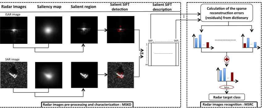
We illustrate inFigure 1the working mechanism of the proposed method (MSKD-MSRC). It is composed by three complementary steps. The first and the second steps include the pre-processing and the characterization using MSKD method. The last step is dedicated to the recognition task using the MSRC classifier. These steps are detailed in the next subsections.
Radar Images Saliency map Salient region
ISAR image
SKP1 ………... SKPk
…
.…………
..……
1
m
………
Radar images pre-processing and characteriza7on : MSKD Radar images recogni7on : MSRC
Calcula7on of the sparse reconstruc7on errors (residuals) from dic7onary
… …
………
…
Min
Radar target class OR
…
SAR image
Salient SIFT
detec7on Salient SIFT descrip7on
Figure 1.Flowchart of the proposed ATR approach: MSKD-MSRC.
2.1. Radar images pre-processing and characterization: MSKD
As mentioned above, we combine the saliency map and SIFT descriptor in order to compute the MSKD for the radar images.
2.1.1. Saliency Attention
The human visual system (HVS) can automatically locate the salient regions on visual images. Inspired by the HVS mechanism, several saliency models are proposed to better understand how the attentional parts regions on images are selected. The most used model in the literature is that proposed by Itti et al. [7]. It locates well the salient regions on an image that visually attract the observers. To achieve this goal, this model exploits three channels: intensity, color and orientation. In this work, we do not integrate the color information using this model due to the grayscale nature of SAR and ISAR images. Based on the intensity channel, this model creates a Gaussian pyramidI(σ), where 0≤σ≤8. To obtain the orientation channel from the intensity images, the model applies a pyramid of oriented Gabor filtersO(σ,θ), whereθ∈ {0◦, 45◦, 90◦, 135◦}is the orientation angles for each level of pyramid. After that, the feature maps (FM) of each channel are computed using the center-surround difference ( ) between a center fine scalec ∈ {2, 3, 4}and a surround coarser scales = c+µ,µ ∈ {3, 4}as following:
• Intensity:
I(c,s) =| I(c) I(s)| (1)
• Orientation:
2.1.2. Scale Invariant Feature Transform (SIFT)
The scale invariant feature transform (SIFT) is a local method proposed by Lowe [17] to extract a set of descriptors from an image. This method has found a widespread use in different image processing applications [34–36]. The SIFT algorithm mainly covers four complementary steps: • Scale space extrema detection: The image is transformed to a scale space by the convolution of
the imageI(x,y)with the Gaussian kernelG(x,y,σ):
L(x,y,σ) =G(x,y,σ)∗I(x,y) (3) whereσis the standard deviation of the Gaussian probability distribution function.
The difference of Gaussian (DOG) is computed as follows:
DOG(x,y,σ) =L(x,y,pσ)−L(x,y,σ) (4) wherepis a factor to control the subtraction between two nearby scales. A pixel in the DOG scale space is considered as local extremum if it is the minimum or maximum of its 26 neighbors pixels (8 neighbors in the current scale and 9 neighbors in the adjacent scale separately).
• Unstable keypoints filtering: The found keypoints in the previous step are filtered to preserve the best candidates. Firstly, the algorithm rejects the keypoints with a DOG value less than a threshold, because these keypoints are with low contrast. Secondly, to discard the keypoints that are poorly localized along an edge, this algorithm uses a Hessian matrix of size 2×2:
H=
"
Dxx Dxy Dxy Dyy
#
(5)
We noteγ2≥1 the ratio between the larger and the smaller eigenvalues of the matrixH. Then,
the method eliminates the keypoints that satisfying: Tr(H)2
Det(H) ≥
γ2+1
γ2 (6)
whereTr(.)is the trace andDet(.)is the determinant.
• Orientation assignment: By selecting a region, we calculate the magnitude and the orientation of each keypoint. After that, a histogram of 36 bins weighted by a Gaussian and the gradient magnitude is built covering the 360 degree range of orientations. The orientation that achieves the peak of this histogram is assigned to the keypoint.
• Keypoint description: To generate the descriptor of each keypoint, we consider a neighboring region around the keypoint. This region has a size of 16×16 pixels and are divided to 16 blocks of size 4×4 pixels. For each block, a weighted gradient orientation histogram of 8 bins are computed. The descriptor is therefore composed by 4×4×8=128 values.
2.1.3. Multi salient keypoints descriptors (MSKD)
background and target areas. An example of this segmentation is illustrated in the third column of the
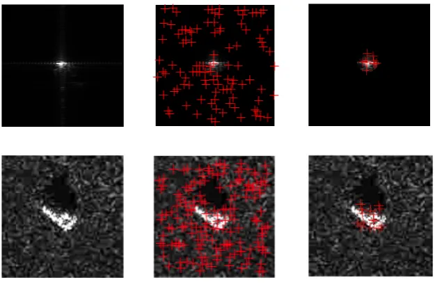
Figure 1. From the segmented radar image, we compute the SIFT keypoints. In this way, we filter out
the keypoints located in the background region as illustrated in the third column ofFigure 2. Finally, the descriptors matrix of one radar image is expressed as:
MSKD=
SKP1 . . . SKPk
1 v1,1 . . . vk,1
..
. ... . .. ... m v1,m . . . vk,m
(7)
wherekis the number of salient keypoints (SKP) in the radar image andmis the size of the descriptor of each SKP which is equals in our work to 128 values.
Figure 2.SIFT and MSKD keypoints distribution. First column: ISAR and SAR images. Second column: SIFT keypoints distribution. Third column: MSKD keypoints distribution.
2.2. Radar images recognition: MSRC
2.2.1. Dictionary construction
The dictionaryAis obtained by the concatenation of all computed MSKD of training radar images as follows:
A= [MSKD1, . . . , MSKDs]
=
SKP1 . . . SKPn
1 v1,1 . . . vn,1
..
. ... . .. ... m v1,m . . . vn,m
(8)
wheresis the number of training radar images. We mention that the number of salient keypoints (SKP) differs from a radar image to another. Assume thatnis the number of SKP in all training radar images, then, the size of the dictionaryAism×nvalues.
2.2.2. Recognition via multitask sparse framework
Given a radar image to recognize, we compute from it the set of local descriptors using the MSKD method:
Y= [y1, ...,yk] (9)
To recognizeYin sparse framework, we should compute the sparse reconstruction errors (residuals) for each taskyi. After that, its class is found according to its sparse linear representation with all training samples:
Y=A.X (10)
withX= (x1, . . . ,xn)∈Rn×kis the sparse coefficient matrix. To obtain it, the following optimization problem is solved as follows:
ˆ X=min
X k
∑
i=1
kxik1subject tokY−AXk2≤e (11)
wherek.k1andk.k2are respectively thel1-norm and thel2-norm.edenotes the error tolerance. The
Equation 11represents a multitask problem since X and Y have multiple atoms (columns). This can be
transformed tok l1-optimization problem, one for eachyi(each task): ˆ
xi=minx i
kxk1subject tokyi−Axik2≤e (12)
Equation 12can be efficiently solved via second-order cone programming (SOCP) [37]. After obtaining
the sparsest matrix ˆX = (xˆ1, . . . , ˆxk), the total reconstruction error of each task for each class is
computed as follows:
rc(yi) =kyi−yiˆk2 =kyi−Aδc(xiˆ)k2
(13)
wherec={1, . . . ,nc}is the labels of classes,ncrepresents the number of classes andδc:Rn→Rnis the characteristic function that selects only the coefficients associated with thec-thclass and set all others to be zero.
After that, the sum fusion is applied among all reconstruction residuals of all tasks according to thenc classes. Finally, the MSRC decides the class of the test sample as the class that produces the lowest total reconstruction error:
class(Y) =min c
k
∑
i=1
3. Experimental results
In this section, we demonstrate the effectiveness of the proposed approach by conducting numerical recognition results on two radar images databases. The first one is composed by ISAR images and the second contains SAR images. To the best of our knowledge, until now there is not a generic approach proposed in the literature having the ability to recognize with the same treatment the ISAR and SAR images except our previous work [16]. That is why aside from our MSKD-MSRC, we also implement two ART methods which are practically close to our method for a fair comparison. The first one uses the SIFT with matching (SIFT+matching). The second one consists on using the MSKD method in combination with the matching (MSKD+matching). We note that the performance of the ATR system is related to its capabilities to locate (ROI) containing the potential targets and its ability to provide a high recognition rate from the signature of the targets.
3.1. Experiment on ISAR images
3.1.1. Database description
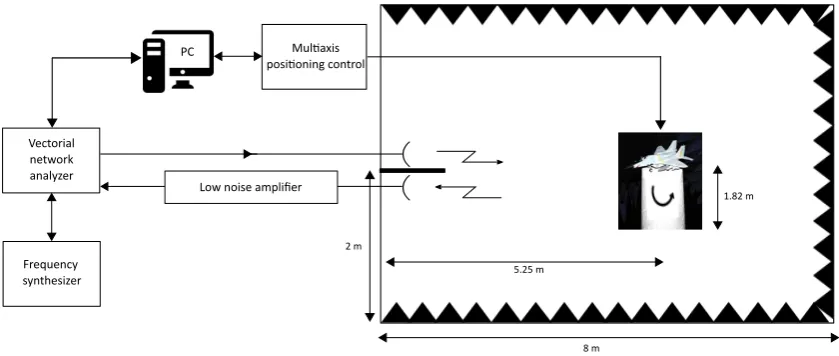
The ISAR images used in our work was acquired in the anechoic chamber of ENSTA Bretagne (Brest, France). The experimental setup of this chamber is depicted inFigure 3. The radar targets are illuminated with a frequency-stepped signal with a band varying between 11.65 GHz and 18 GHz. A sequence of pulses is emitted using a frequency increment∆f =50 MHz. By applying the inverse fast Fourier transform (IFFT), we obtain 162 grayscale images per class with a size of 256×256 pixels. To construct the ISAR database images, we have used 12 reduced aircraft models with 1/48 reduced scale. For each target class, 162 ISAR images are generated. Consequently, the total number of ISAR images in this database is 1944. For a rigorous details about the experiments conducted on the anechoic chamber, the reader is refereed to [1,38]. Samples of each aircraft target class of this dataset are displayed inFigure 4.
Mul�axis posi�oningcontrol
Vectorial network analyzer
Frequency synthesizer
PC
Lownoiseamplifier 1.82m
2m
5.25m
8m
Figure 3.Experimental setup of the anechoic chamber.
3.1.2. Target recognition results
A10 F4 F14 F15
F16 F18 F104 F117
Harrier Mig29 Rafale Tornado
Figure 4.Twelve classes of ISAR database.
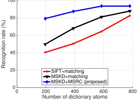
method outperforms the remaining ones under the different considered number of dictionary atoms. Additionally, comparing the matching and the MSRC to recognize the MSKD, it is observed that with the decreasing number of atoms, the recognition rate of MSKD+matching descends faster than that of the proposed method. In the upcoming experiments, we adopt 780 atoms. The comparison in term of the overall recognition rate is given inTable 1where the best accuracy are highlighted in bold. According to this table, some observations are concluded. First, the SIFT method provides the worst result. That is due to the location of keypoints in the background of the ISAR images which is not necessary for the recognition as illustrated inFigure 2. Contrary, the MSKD contributes to enhance the recognition rate thanks to its concentration of SIFT keypoints in the target area. Then, by considering the matching, with a little number of keypoints of 23559 that corresponds to 17.83% of the 420027 initial keypoints, the recognition rate is improved by 5.29%. This issue demonstrates the benefit of the adopted filtration of the SIFT keypoints. Second, the MSRC performs better than the matching. That can be explained by the fact that the multitask sparsity of the MSKD of ISAR images leads to an enhancement of recognition rate.
0 200 400 600 800
Number of dictionary atoms
0 20 40 60 80 100
Recognition rate (%)
SIFT+matching MSKD+matching MSKD+MSRC (proposed)
Figure 5.Recognition rate variation with the number of dictionary atoms on ISAR images database.
Table 1.Comparison between the recognition rate (%) of different methods on ISAR images database.
Methods SIFT+Matching MSKD+Matching MSKD+MSRC
(proposed)
Recognition 82.61 87.90 93.65
rate
Number of 420 027 23 559 23 559
keypoints
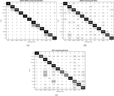
F104, A10, F14 and Mig29. The SIFT+matching gives a high recognition rate comparing to other methods for only one class which is the Rafale. The overall recognition rate of our method is 93.65% which is 11.04% and 5.75% better than SIFT+matching and MSKD+matching methods respectively. This improvement demonstrates the power of the combination of the MSKD and the multitask sparse classifier to recognize the ISAR images.
MSKD+MSRC (proposed) (93.65%)
100 0 0 0 0 0 0 0 0 0 0 0 4.12 95.88 0 0 0 0 0 0 0 0 0 0
0 11.34 88.66 0 0 0 0 0 0 0 0 0
0 0 2.06 95.88 0 0 0 1.03 0 0 0 1.03
0 0 0 0 100 0 0 0 0 0 0 0
0 0 0 0 0 100 0 0 0 0 0 0
0 0 0 0 0 0 100 0 0 0 0 0
0 0 0 0 0 0 28.57 71.43 0 0 0 0
0 0 0 0 0 0 0 3.09 96.91 0 0 0
0 0 0 0 0 0 0 0 0 100 0 0
0 0 0 0 0 0 0 0 0 23.71 76.29 0
0 0 0 0 0 0 0 0 0 1.03 0 98.97
F117 Harrier Rafale Tornado F104 A10 F14 F15 F16 Mig29 F18 F4 Prediction (%) F117 Harrier Rafale Tornado F104 A10 F14 F15 F16 Mig29 F18 F4 Truth (a) MSKD+matching (87.90%)
97.94 0 2.06 0 0 0 0 0 0 0 0 0 0 94.85 0 0 0 0 3.09 0 0 1.03 1.03 0 0 9.28 85.57 0 0 0 1.03 0 0 0 0 4.12 4.12 3.09 3.09 82.47 2.06 2.06 1.03 1.03 0 1.03 0 0
0 0 4.12 2.06 87.63 0 2.06 1.03 0 1.03 0 2.06 3.09 0 0 2.06 0 92.78 2.06 0 0 0 0 0
0 3.06 4.08 0 1.02 4.08 85.71 0 0 2.04 0 0 0 0 0 3.06 0 0 2.04 91.84 0 3.06 0 0 0 0 1.03 2.06 1.03 0 2.06 3.09 90.72 0 0 0 0 1.03 0 0 0 0 4.12 0 1.03 89.69 4.12 0 0 11.34 0 2.06 1.03 2.06 2.06 3.09 1.03 2.06 74.23 1.03 0 5.15 0 6.19 2.06 0 1.03 1.03 0 3.09 0 81.44
F117 Harrier Rafale Tornado F104 A10 F14 F15 F16 Mig29 F18 F4 Prediction (%) F117 Harrier Rafale Tornado F104 A10 F14 F15 F16 Mig29 F18 F4 Truth (b) SIFT+matching (82.61%)
100 0 0 0 0 0 0 0 0 0 0 0 2.74 74.66 2.74 2.05 0.68 0.68 1.37 1.37 1.37 6.85 0.68 4.79
0 0 98.62 0 0 0 0 0 0 0.69 0.69 0 0 0 0.68 93.84 0 0 0 0 1.37 4.11 0 0 0 0 2.05 0 94.52 0 0 0 0 0.68 2.74 0 0 0 2.74 0 5.48 86.30 2.05 0 0 3.42 0 0 0 0 19.18 0 7.53 0.68 64.38 0.68 0 0.68 0.68 6.16 0 0 23.97 0 7.53 1.37 0.68 53.42 0 3.42 2.05 7.53 0 0 0 0.68 0 0 0 0 99.32 0 0 0
0 0 0 0 21.23 0 0 0 0 64.38 4.79 9.59
0 0 0.69 0 2.76 1.38 1.38 0 0 11.72 80.00 2.07
0 0 4.14 2.76 1.38 0.69 0 0 0 8.97 0 82.07
F117 Harrier Rafale Tornado F104 A10 F14 F15 F16 Mig29 F18 F4 Prediction (%) F117 Harrier Rafale Tornado F104 A10 F14 F15 F16 Mig29 F18 F4 Truth (c)
Figure 6.Confusion matrix of the different methods on ISAR images database: : (a) MSKD+MSRC; (b)
3.2. Experiments on SAR images
3.2.1. Databases description
Regarding to the SAR images, the moving and stationary target acquisition and recognition (MSTAR) public dataset1is used. This last is developed by Air Force Research Laboratory (AFRL) and the Defense Advanced Research Projects Agency (DARPA). The SAR images in this dataset are gathered by the X-band SAR sensor in spotlight mode. The MSTAR dataset includes multiple ground targets. Samples of each military ground target class of this dataset are displayed inFigure 7. Two
T62 T72 BRDM2 BMP2
BTR60 BTR70 2S1 D7
ZIL131 ZSU234
Figure 7.Ten classes of MSTAR database: two tanks (T62 and T72), four armored personnel carriers (BRDM2, BMP2, BTR60 and BTR70), a rocket launcher (2S1), a bulldozer (D7), a truck (ZIL131), and an Air Defence Unit (ZSU234).
major versions are available for this dataset:
• SAR images under standard operating conditions (SOC, seeTable 2). In this version, the training SAR images are obtained at the 17◦depression angle and the test ones at 15◦depression angle. Then, there is a depression angle difference of 2◦.
• SAR images under extended operating conditions (EOC) including:
– The configuration variations (EOC-1, seeTable 3). The configuration refers to small structural modifications and physical difference. Similarly to the SOC version, the training and the test targets are captured at 17◦and 15◦depressions angles respectively.
– The depression variations (EOC-2, seeTable 4). The SAR images acquired at 17◦depression angle are exploited for training, while the ones taken at 15◦, 30◦and 45◦depressions angles are used for testing.
The main difference between the SOC and EOC versions is that in the SOC, the condition of training and test sets are very near contrary to the EOC. We note that in the opposite case of the ISAR images database, the MSTAR is already partitioned to training and test datasets.
3.2.2. Target recognition results
We provide inTable 5the quantitative comparison between the different methods on several version of MSTAR dataset. As can be seen from this table, the MSKD performs much better than the use of the whole SIFT keypoints. The reason is that not all SIFT keypoints are useful to characterize the SAR images, and it can be remedied by the the adopted filtration method as illustrated inFigure 2. This
Table 2.Number of SAR images in MSTAR database under SOC.
Target classes Depression angle
17◦(train) 15◦(test)
T62 299 273
T72 232 196
BRDM2 298 274
BMP2 233 195
BTR60 256 195
BTR70 233 196
2S1 299 274
D7 299 274
ZIL131 299 274
ZSU234 299 274
Total 2747 2425
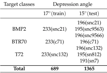
Table 3. Number of SAR images in MSTAR database under configuration variation: EOC-1. The content in bracket represents the serial number of configuration.
Target classes Depression angle
17◦(train) 15◦(test)
196(snc21)
BMP2 233(snc21) 195(snc9563)
196(snc9566)
BTR70 233(c71) 196(c71)
196(snc132)
T72 233(snc132) 195(sn812)
191(sn7)
Total 689 1365
Table 4.Number of SAR images in MSTAR database under depression variation: EOC-2.
Target classes Depression angle
Train Test
17◦ 15◦ 30◦ 45◦
2S1 299 274 288 303
BRDM2 298 274 420 423
ZSU234 299 274 406 422
Total 896 822 1114 1148
conclusion in an important motivation for coupling the saliency attention and the SIFT. Additionally, the use of the multitask SRC leads to an overwhelming superiority compared to the matching approach thanks to the sparse vectors extracted from each task in the MSKD.
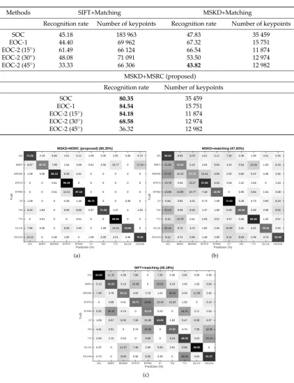
Considering the 10-class ground target (SOC), the recognition rate of the proposed method is 80.35% which is 35.17% and 32.52% better than the SIFT+matching and the MSKD+matching. The confusion matrix of all methods are displayed inFigure 8. The proposed method provides a confusion between the BMP2, BRDM2 and BTR70 targets because they have the same vehicle type which is the armored personnel carriers. It does not able to classify correctly the BMP2 target. However, it has the high recognition rates for all classes compared to the remaining methods.
Table 5.Comparison between the recognition rate (%) of different methods on MSTAR dataset.
Methods SIFT+Matching MSKD+Matching
Recognition rate Number of keypoints Recognition rate Number of keypoints
SOC 45.18 183 963 47.83 35 459
EOC-1 44.40 69 962 67.32 15 751
EOC-2 (15◦) 61.49 66 124 66.54 11 874
EOC-2 (30◦) 48.08 71 091 53.50 12 974
EOC-2 (45◦) 33.33 66 306 43.82 12 982
MSKD+MSRC (proposed)
Recognition rate Number of keypoints
SOC 80.35 35 459
EOC-1 84.54 15 751
EOC-2 (15◦) 84.18 11 874
EOC-2 (30◦) 68.58 12 974
EOC-2 (45◦) 36.32 12 982
MSKD+MSRC (proposed) (80.35%)
73.36 2.19 5.84 4.01 5.11 1.09 0.36 2.92 0.36 4.74 6.67 49.74 7.69 1.54 3.08 0.51 2.56 10.77 0 17.44 1.09 0.36 86.13 8.39 4.01 0 0 0 0 0
0 0 0.51 99.49 0 0 0 0 0 0
0 0 0.51 12.31 87.18 0 0 0 0 0
1.09 0 0 0.36 1.46 96.72 0 0 0.36 0 8.42 1.83 0 6.59 8.06 0.37 71.43 1.47 0 1.83
0 0.51 0 0 0.51 0 0 98.98 0 0
7.66 0.36 0 8.39 3.65 0 1.09 14.23 64.60 0
13.14 0 0.36 1.82 0 1.09 3.28 4.01 0.36 75.91
2S1 BMP2 BRDM2 BTR70 BTR60 D7 T62 T72 ZIL131 ZSU234 Prediction (%) 2S1 BMP2 BRDM2 BTR70 BTR60 D7 T62 T72 ZIL131 ZSU234 Truth (a) MSKD+matching (47.83%)
55.84 6.93 8.76 4.01 5.11 7.30 4.38 1.09 4.01 2.55 21.54 34.36 6.15 2.05 5.64 4.10 5.64 13.33 1.03 6.15 27.37 10.22 27.74 12.41 6.93 2.92 3.65 5.47 0.36 2.92 13.78 2.55 13.27 57.65 6.63 2.04 1.02 1.53 0 1.53 13.85 13.85 10.77 7.18 42.05 0 2.05 5.64 1.54 3.08 5.84 3.65 4.01 0.73 1.09 71.53 3.28 0.73 2.92 6.20 20.15 6.59 8.42 1.47 1.83 6.59 40.29 2.56 2.56 9.52 8.16 13.78 0.51 2.55 3.57 3.57 3.06 60.20 1.02 3.57 20.44 8.76 4.74 1.82 2.92 10.95 4.01 4.01 39.42 2.92 9.12 4.74 5.84 1.46 2.55 9.12 8.03 4.38 4.74 50.00
2S1 BMP2 BRDM2 BTR70 BTR60 D7 T62 T72 ZIL131 ZSU234 Prediction (%) 2S1 BMP2 BRDM2 BTR70 BTR60 D7 T62 T72 ZIL131 ZSU234 Truth (b) SIFT+matching (45.18%)
64.60 11.31 4.38 7.66 0 7.30 0.36 3.65 0.36 0.36 5.13 41.03 5.13 15.38 0 20.51 5.13 1.03 1.03 5.64 7.58 3.79 35.23 4.55 3.79 1.52 26.52 3.03 11.36 2.65 0 4.08 0.51 35.71 30.61 12.24 10.20 1.53 0 5.10 6.32 26.32 4.74 0 33.16 0.53 0 24.21 2.11 2.63 1.09 6.57 8.03 7.30 10.95 43.80 1.82 5.47 8.39 6.57
4.41 5.51 0 0.74 25.00 0 37.87 0.74 7.35 18.38
2.69 2.15 0.54 0 9.68 0 9.14 48.39 3.23 24.19 0.37 0 11.57 7.46 2.99 5.60 2.61 8.58 60.82 0
0.73 0 9.09 0.36 6.55 0.36 0 28.00 3.64 51.27
2S1 BMP2 BRDM2 BTR70 BTR60 D7 T62 T72 ZIL131 ZSU234 Prediction (%) 2S1 BMP2 BRDM2 BTR70 BTR60 D7 T62 T72 ZIL131 ZSU234 Truth (c)
Figure 8.Confusion matrix of the different methods on MSTAR dataset under SOC: (a) MSKD+MSRC;
(b) MSKD+matching; (c) MKD+matching
Table 6.Comparison between the confusion matrix (%) of different methods on MSTAR dataset under EOC-1 (configuration variation).
SIFT+Matching (44.40) MSKD+Matching (67.32) MSKD+MSRC (proposed) (84.54)
BMP2 BTR70 T72 BMP2 BTR70 T72 BMP2 BTR70 T72
BMP2 80.58 0 19.42 52.98 5.96 41.06 72.06 8.35 19.59
BTR70 53.57 0 46.42 10.20 82.14 7.65 1.02 98.98 0
T72 77.14 0 22.85 20.27 2.92 76.80 6.35 1.37 92.26
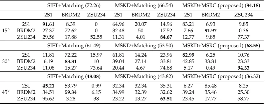
For the depression variations (EOC-2), the recognition rate is sharply degraded when the aspect angle increases for all methods. That is due to the variation between the aspect angles especially in the case of 30◦and 45◦which represent a change of 13◦and 28◦compared to the train targets captured at 17◦. For instance, using the proposed method drops from 84.18% to 68.58% to 36.32%. The recognition rate of MSKD-MSRC still achieves the highest recognition rate in 15◦ and 30◦ depression angles. Whereas, the SIFT+Matching and the MSKD+Matching work better in the case of 45◦ depression angle.Table 7records the confusion matrix of all methods under EOC-2 using different depression angles. The proposed method gives a balanced recognition rate per class with a low value of the misclassification. However, for the 45◦depression angle, we show a high confusion between BRDM2 and 2S1 which drastically degrades the overall recognition rate. Similarly, the 30◦depression angle enjoys the trend with a more moderation to 45◦depression angle.
Table 7.Comparison between the confusion matrix of different methods (%) on MSTAR dataset under EOC-2 (depression variation).
SIFT+Matching (72.26) MSKD+Matching (66.54) MSKD+MSRC (proposed) (84.18)
2S1 BRDM2 ZSU234 2S1 BRDM2 ZSU234 2S1 BRDM2 ZSU234
2S1 91.61 8.39 0 64.96 20.07 14.96 83.21 6.93 9.85
15◦ BRDM2 27.37 72.62 0 32.48 50 17.52 7.66 91.97 0.36
ZSU234 29.56 17.88 52.55 11.31 4.01 84.67 12.77 9.85 77.37
SIFT+Matching (61.49) MSKD+Matching (53.50) MSKD+MSRC (proposed) (68.58)
2S1 11.81 72.22 15.97 61.81 14.24 23.96 82.99 6.25 10.76
30◦ BRDM2 6.19 83.81 10 39.04 27.14 33.81 42.85 33.81 23.33
ZSU234 11.08 15.27 73.64 20.44 4.67 74.88 5.17 0.49 94.33
SIFT+Matching (48.08) MSKD+Matching (43.82) MSKD+MSRC (proposed) (36.32)
2S1 45.21 53.79 0.99 32.34 32.34 35.31 6.27 85.48 8.25
45◦ BRDM2 34.51 59.34 6.15 34.99 32.39 32.62 39.24 35.46 25.30
ZSU234 95.62 3.28 38 23.22 13.27 63.51 23.45 17.77 58.77
4. Conclusions and Future Work
classes, it achieves in most cases the high overall recognition rates with a balanced performance for all ISAR and SAR classes in a reasonable runtime. Additionally, it effectively deals with the challenge of target recognition under EOC with a slight degradation in the case of EOC-2 (45◦). Considering the minor flaws of the proposed method, the future work will focus on using other local descriptors as well as testing the proposed system in other radar images databases such as those acquired in the maritime environment.
Conflicts of Interest:The authors declare no conflict of interest
References
1. Toumi, A.; Khenchaf, A.; Hoeltzener, B. A retrieval system from inverse synthetic aperture radar images:
Application to radar target recognition. Information Sciences2012,196, 73–96.
2. El-Darymli, K.; Gill, E.W.; Mcguire, P.; Power, D.; Moloney, C. Automatic Target Recognition in Synthetic
Aperture Radar Imagery: A State-of-the-Art Review. IEEE Access2016,4, 6014–6058.
3. Toumi, A.; Hoeltzener, B.; Khenchaf, A. Hierarchical segmentation on ISAR image for target recongition.
International Journal of Computational research2009,5, 63–71.
4. Bolourchi, P.; Demirel, H.; Uysal, S. Target recognition in SAR images using radial Chebyshev moments.
Signal, Image and Video Processing2017,11, 1033–1040.
5. Ding, B.; Wen, G.; Ma, C.; Yang, X. Decision fusion based on physically relevant features for SAR ATR.IET
Radar, Sonar Navigation2017,11, 682–690.
6. Chang, M.; You, X. Target Recognition in SAR Images Based on Information-Decoupled Representation.
Remote Sensing2018,10.
7. Itti, L.; Koch, C.; Niebur, E. A model of saliency-based visual attention for rapid scene analysis. IEEE
Transactions on Pattern Analysis and Machine Intelligence1998,20, 1254–1259.
8. Kumar, N. Thresholding in salient object detection: a survey.Multimedia Tools and Applications2017.
9. Borji, A.; Itti, L. State-of-the-Art in Visual Attention Modeling.IEEE Transactions on Pattern Analysis and
Machine Intelligence2013,35, 185–207.
10. Gao, F.; You, J.; Wang, J.; Sun, J.; Yang, E.; Zhou, H. A novel target detection method for SAR images based
on shadow proposal and saliency analysis. Neurocomputing2017,267, 220 – 231.
11. Wang, Z.; Du, L.; Zhang, P.; Li, L.; Wang, F.; Xu, S.; Su, H. Visual Attention-Based Target Detection and
Discrimination for High-Resolution SAR Images in Complex Scenes.IEEE Transactions on Geoscience and
Remote Sensing2017,PP, 1–18.
12. Diao, W.; Sun, X.; Zheng, X.; Dou, F.; Wang, H.; Fu, K. Efficient Saliency-Based Object Detection in Remote
Sensing Images Using Deep Belief Networks. IEEE Geoscience and Remote Sensing Letters2016,13, 137–141.
13. Song, H.; Ji, K.; Zhang, Y.; Xing, X.; Zou, H. Sparse Representation-Based SAR Image Target Classification
on the 10-Class MSTAR Data Set. Applied Sciences2016,6.
14. Dong, G.; Kuang, G. A Soft Decision Rule for Sparse Signal Modeling via Dempster-Shafer Evidential
Reasoning.IEEE Geoscience and Remote Sensing Letters2016,13, 1567–1571.
15. Dong, G.; Kuang, G.; Wang, N.; Zhao, L.; Lu, J. SAR Target Recognition via Joint Sparse Representation
of Monogenic Signal.IEEE Journal of Selected Topics in Applied Earth Observations and Remote Sensing2015,
8, 3316–3328.
16. Karine, A.; Toumi, A.; Khenchaf, A.; Hassouni, M.E. Target Recognition in Radar Images Using Weighted
Statistical Dictionary-Based Sparse Representation. IEEE Geosci. Remote Sensing Lett.2017,14, 2403–2407.
17. Lowe, D. Distinctive Image Features from Scale-Invariant Keypoints. International Journal of Computer
Vision2004,60, 91–110.
18. Zhu, X.; Ma, C.; Liu, B.; Cao, X. Target classification using SIFT sequence scale invariants.Journal of Systems
Engineering and Electronics2012,23, 633–639.
19. Agrawal, A.; Mangalraj, P.; Bisherwal, M.A. Target detection in SAR images using SIFT. 2015 IEEE
International Symposium on Signal Processing and Information Technology (ISSPIT), 2015, pp. 90–94.
20. Karine, A.; Toumi, A.; Khenchaf, A.; Hassouni, M.E. Target detection in SAR images using SIFT. 2017
21. Jdey, I.; Toumi, A.; Khenchaf, A.; Dhibi, M.; Bouhlel, M. Fuzzy fusion system for radar target recognition.
International Journal of Computer Applications & Information Technology2012,1, 136–142.
22. Sun, Y.; Liu, Z.; Todorovic, S.; Li, J. Adaptive boosting for SAR automatic target recognition. IEEE
Transactions on Aerospace and Electronic Systems2007,43, 112–125.
23. Huang, Z.; Pan, Z.; Lei, B. Transfer learning with deep convolutional neural network for SAR target
classification with limited labeled data. Remote Sensing2017,9, 907.
24. El Housseini, A.; Toumi, A.; Khenchaf, A. Deep Learning for target recognition from SAR images. Detection
Systems Architectures and Technologies (DAT), Seminar on. IEEE, 2017, pp. 1–5.
25. Wright, J.; Yang, A.Y.; Ganesh, A.; Sastry, S.S.; Ma, Y. Robust face recognition via sparse representation.
IEEE transactions on pattern analysis and machine intelligence2009,31, 210–227.
26. Li, W.; Du, Q. A survey on representation-based classification and detection in hyperspectral remote
sensing imagery. Pattern Recognition Letters2016,83, 115 – 123. Advances in Pattern Recognition in Remote
Sensing.
27. Xing, X.; Ji, K.; Zou, H.; Chen, W.; Sun, J. Ship Classification in TerraSAR-X Images With Feature Space
Based Sparse Representation. IEEE Geoscience and Remote Sensing Letters2013,10, 1562–1566.
28. Samadi, S.; Cetin, M.; Masnadi-Shirazi, M.A. Sparse representation-based synthetic aperture radar imaging.
IET Radar, Sonar Navigation2011,5, 182–193.
29. Chang, M.; You, X. Target Recognition in SAR Images Based on Information-Decoupled Representation.
Remote Sensing2018,10, 138.
30. Yu, M.; Dong, G.; Fan, H.; Kuang, G. SAR Target Recognition via Local Sparse Representation of
Multi-Manifold Regularized Low-Rank Approximation.Remote Sensing2018,10, 211.
31. Wang, X.; Shao, Z.; Zhou, X.; Liu, J. A novel remote sensing image retrieval method based on visual salient
point features.Sensor Review2014,34, 349–359.
32. Liao, S.; Jain, A.K.; Li, S.Z. Partial Face Recognition: Alignment-Free Approach. IEEE Transactions on
Pattern Analysis and Machine Intelligence2013,35, 1193–1205.
33. Zhang, L.; Ding, Z.; Li, H.; Shen, Y.; Lu, J. 3D face recognition based on multiple keypoint descriptors and
sparse representation. PloS one2014,9, e100120.
34. Zhou, D.; Zeng, L.; Liang, J.; Zhang, K. Improved method for SAR image registration based on scale
invariant feature transform. IET Radar, Sonar Navigation2017,11, 579–585.
35. Bai, C.; nan Chen, J.; Huang, L.; Kpalma, K.; Chen, S. Saliency-based multi-feature modeling for semantic
image retrieval. Journal of Visual Communication and Image Representation2018,50, 199 – 204.
36. Yuan, J.; Liu, X.; Hou, F.; Qin, H.; Hao, A. Hybrid-feature-guided lung nodule type classification on CT
images. Computers & Graphics2018,70, 288 – 299. CAD/Graphics 2017.
37. Candes, E.; Romberg, J. l1-magic: Rrrecovery of sparse signals via convex programming. Technical Report
(California Institute of Technology)2007.
38. Bennani, Y.; Comblet, F.; Khenchaf, A. RCS of Complex Targets: Original Representation Validated by
Measurements-Application to ISAR Imagery. IEEE Transactions on Geoscience and Remote Sensing2012,