New Mathematical Approach for Economic Power Dispatch Problem with Quadratic Objective Function

ISSN (e): 2250-3021, ISSN (p): 2278-8719

Vol. 09, Issue 6 (June. 2019), ||S (IV) || PP 25-30

New Mathematical Approach for Economic Power Dispatch

Problem with Quadratic Objective Function

S. Kavitha

1

, Nirmala P. Ratchagar

2

1

Assistant Professor, Department of Mathematics, Annamalai University, Chidambaram-608001, India

2_{Professor, Department of Mathematics, Annamalai University, Chidambaram-608001, India}

Corresponding Author: S. Kavitha

Abstract: A new mathematical approach is proposed for the solution of optimization problem with quadratic

objective function subject to satisfying equality and inequality constraints. The convergence of the conventional lambda iteration method is improved by the superlinear bracketing method. Lambda value is updated in each iteration by the superlinear bracketing method. The practical application of the proposed method is illustrated with economic power dispatch problem. Economic power dispatch problem is one of the fundamental issues in an electrical power system operation. It is a nonlinear optimization problem and their objective is to minimize the total fuel cost of a thermal power generating units subject to satisfying various operating constraints. The proposed mathematical approach is implemented for the solution of economic power dispatch problem. The result shows that the proposed method provides the optimal solution and it requires lesser number of iterations for the convergence.

--- --- Date of Submission: 11-06-2019 Date of acceptance: 27-06-2019

---I.

INTRODUCTION

The numerous mathematical methods are developed in the literature to find solution for the optimization problem with quadratic objective function. There are several disadvantages of these methods for finding solution for the non-linear optimization problem. In λ-iteration method, suitable initial value must be selected and this method needs more number of iterations for the convergence.

Similarly, gradient, dynamic programming and quadratic programming have certain difficulties to solve this problem. The computational difficulty is prominent in dynamic programming approach which is referred as the curse of dimensionality[1-4]. Mullers method[5], Brent’s method[6], Bisection method[7], Regula-falsi[8], Bracketing method[9] were developed in the literature to solve the nonlinear equations. Recently, Superlinear bracketing method[10] is reported in the literature to solve the nonlinear equations. The Superlinear bracketing method is able to find the roots for the nonlinear equations on the given interval.

A new method based on superlinear bracketing approach is proposed to find the solution of quadratic objective function with equality and inequality constraints. The lambda value of lagragian multiplier method is updated using the superlinear bracketing method[10]. The problem considered in this paper resembles the practical economic power scheduling problem in an electrical power system[11]. Economic power dispatch is the important optimization problem in thermal power stations. The solution of this problem gives the optimal power generation schedule of the committed electrical generators that minimize the total fuel cost subject to satisfying the equality and inequality constraints[12]. The equality constraint is the total power generation should be equal to total power demand and transmission losses. The inequality constraints are the power generation of the committed generating units should lie within the operating limits.

II.

PROBLEM FORMULATION

The objective function of the optimization problem is formulated by Min ZF(X), the objective is expressed as the sum of n single-variable function F1(x1), F2(x2), …, Fn(xn). i .e, F(x1, x2, … ,xn) =

F1(x1)+F2(x2)+ … + Fn(xn ). The minimization objective function is stated as



  n 1 i

i F Z

Min (xi) (1)

where Fi(xi) is quadratic function. It is defined as

_F

₍

x

₎



a

_i

x

_i2



b

_i

x

_i



c

_i i

i (2)

ai, bi, and ci are coefficients of decision variable xi, and n is the total number of variables. The above objective is

(i) Equality constraint _{X X} L n 1 i T 



 i

x (3)

where XT is fixed value and nonlinear equation XL is given by

00 n 1 i 0i ij n 1 i n 1 j

L A A A

X





  

 

 x_i x_j x_i (4)

The coefficients Aij, A0i and A00 are constants and Aij is a symmetrical matrix.

(ii) Inequality constraint

x

_imin



x

_i



x

_imax, for i = 1, 2, … , n (5)

where

x

_im inand

x

_imaxare the lower and upper limits of the ith decision variable.

(iii) Non negativity constraint

_xi_0, for i = 1, 2, … , n (6)

III. COMPUTATIONAL PROCEDURE

The equality constraint is added with objective function using lagrangian multiplier λ,

_{(x ) x )}

i i L n 1 i T n 1 i

i -λ ( X X F

Z





 

 

(7)

Therefore

_{(ax bx c) x )}

i i i i i i L n 1 i T n 1 i X X ( λ

-Z



 



 

 

2 (8)

Differentiating the equation (8) with respect to control variable xi and then equated to zero.

That is, _0  

i

x

Z ₍₉₎

₂

₍

_2A

_A

₎

_λ

0i j n 1 j ij









 

x

x

a

b

_{i i i}



(10)

₂

₂

_A

₍

_2A

_A

₎

_λ

0i j n i j 1 j ij i

ii











  

x

x

x

a

b

_{i i i}





(11)

By rearranging, we get

λ

A

2A

λ

-λ

)

A

(

2

n _{j 0i}

i j1 j ij

ii













 i

i

i

a

x

b

x



(12)

Hence ) A ( 2 A λ 2 ) A 1 ( ii j n i j 1 j ij 0i           i i i a x b x

for i = 1, 2, … , n (13) and ) A 2A λ 0i j n 1 j ij    



 x ( x a bi i i

1

2 (14)

The computational procedure to calculate the limits of λ for

x

_im in, is given below:

1. Determine the λ value using eqn. (14). In eqn. (14), xi is substituted by

m in

i

x

and xj is substituted by

m in

j

x

.

2. Fix the iteration number k=0. The initial value of of

x

_ik is calculated by

,

2

)

(

_imin _imax k

i

x

x

x





for i = 1, 2, … , n. (15) 3. Calculate

x

_ik1 from the equation (13).

4. Verify the convergence by calculating



x

from the current and previous iterations, i.e. k

i k i

x

x

x





5. Increase the iteration by 1, that is k=k+1. The decision variables calculated in step-3 will be taken as an initial value and new values are calculated using step-3 and check the convergence using step-4.

6. Using equation (14), calculate the λ-value, calculate XT from the following equation,

L n

1 i

T X

X 





 i

x (16)

The computational steps given above is repeated for

x

_imax. Therefore for n-variables, 2n λ-values and their

corresponding XT are computed. The lookup table is prepared by arranging these values in ascending order.

Using the superlinear bracketing method [10], the optimal value of lambda is calculated.

The steps involved to solve the optimization problem described in equations(1) to (6) are detailed below: Step1: For the given value of XT , determine the limits of λ from the look-up Table.

Step 2: Determine the values of variable xi for λ1 and for λ2 using eqn. (13).

Step 3: Calculate the function values f1=f(λ1) using variables xi corresponding to λ1,

i.e

L T n

1 i

1) X X

f( 



 

 i

x

 (17)

and f2=f(λ2) using variables xi corresponding to λ2,

i.e

L T n

1 i

2) X X

f( 



   i

x

 (18)

Step 4: If sign(f1) is equal to sign(f2) then adjust the values of λ1 and λ2 such that sign of f(λ1) is negative and

sign of f(λ2) is positive. Check the initial condition. If sign(f1) == sign(f2) then adjust the values of λ1 and λ2

such that sign of f(λ1) is –ve and sign of f(λ2) is +ve.

Step 5: Set maximum number of iteration ITmax, tolerance ε and iteration counter k1=0. Calculate the initial

mid-point

2

2 1 0







  and the function value f0=f(λ0). Set λm=λ0.

Step 6: Calculate

) -)( -(

f -f )

-)( -(

f -f A

2 1 0 2

2 0 2

1 0 1

0 1

1 _{   }  _{   } (19)

) -)( -(

) -)( f -(f ) -)( -(

) -)( f -(f B

2 1 0 2

0 1 2 0 2 1 0 1

0 2 1 0

1 _{   }

  

  

 



 (20)

0 1 f

C  (21)

Step 7: Determine

1 1 2 1 1 1

1 0

p

C A 4 B ) sgn(B B

C 2

 

 

 (22)

Step 8: If λp>λ2 or λp < λ1 then

1

1 1 2 1 1 1

0 p

A 2

C A 4 B ) sgn(B

B  





 (23)

Step 9: For λp, calculate the values of variables xi using eqn. (13), if xi violates its maximum or minimum then

fix the value of xi to upper or lower limit, repectively, and find the function value fp = f(λp).

Step10: If f1f0 < 0 then λ2 = λ0, f2 = f0 else λ1 = λ0, f1 = f0.

Step 11: Set λ0 = λp, f0 = fp, If k1 > ITmax. then stop.

Step 12: If k1 is greater than 1 and

λ

_m



λ

₀



ε

then print the results λ0, decision variables xi, and f0, and stop.

Step14: Increase the iteration by 1, that is k1= k1 + 1 and update λm=λ0.

Step 15: Go to Step 6.

IV. ECONOMIC POWER DISPATCH PROBLEM

The economic dispatch problem is formulated as

$/h

c P b P a ) (P F Min F

n

i

i i i i i i

n

i i

T





 

  



1 2 1

(24)

subject to

(i) power balance constraints

At a particular dispatch interval (usually 1h), the total generation of committed units must be equal to system load demand PD plus transmission loss PL are met

MW

L D

n

i

i P P

P 



1

(25)

The transmission loss PL is a function of generator’s power output and is calculated using B- matrix loss

formula. The general form of the loss formula using B-coefficients is

MW 00 1 1

0 1 1

B P B P

B P P

n

i n

j i i j

ij n

i n

j i

L 









   

(26)

(ii) generating capacity constraints

The physical restrictions on the real power output of generating units constitute the following constraint

n , , , i i

P i P i

Pmin   max MW 123..., (27)

where min i

P and Pimax are the minimum and maximum power outputs of the ith unit.

V.

RESULT AND DISCUSSION

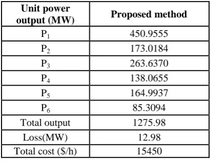
In order to verify the effectiveness of the proposed mathematical approach, a six-generating units sample test system including transmission loss is considered[13]. The operating ranges of all committed generating units are restricted by their minimum and maximum power generation limits. The sample system contains of six thermal generating units. The total load demand of the system is 1263 MW. The cost coefficients, generation limits of each generating unit and transmission loss coefficient are given in Appendix. The proposed approach is applied to sample test system using Matlab 6.5 programming language. The optimal generation schedule obtained through the proposed method minimizes the total fuel cost and satisfies power balance constraint i.e. total output minus loss should be equal to total load demand of the system and other operating constraints. The number of iterations taken by the method for the convergence is four. The optimal solution obtained through the proposed mathematical method is Table 1.

Table 1: Optimal solution obtained through proposed recursive method for the Load demand 1263 MW

Unit power

output (MW) Proposed method

P1 450.9555

P2 173.0184

P3 263.6370

P4 138.0655

P5 164.9937

P6 85.3094

Total output 1275.98

Loss(MW) 12.98

Total cost ($/h) 15450

VI. CONCLUSION

REFERENCES

[1]. C.L.Wadhwa, Electrical Power System. New age international publisher. 2005. [2]. Hadi Sadaat, Power system analysis. Tata McGraw-Hill. 2016.

[3]. R.M.S.Danaraj, F.Gajendran, Quadratic programming solution to emission and economic dispatch problems. Institution of Engineer Journal.2005; 86.

[4]. H.A.Taha, Operation Research: An introduction. Prentice Hall of India. 1997

[5]. R.P.Brent, Algorithms for Minimization Without Derivatives. Englewood Cliffs. NJ: Prentice-Hall. 1973 [6]. I.Barrodale and K.B.Wilson, A Fortran program for solving a nonlinear equation by Muller’s method.

Journal of Computational and Applied Mathematics. 1978; 4(2):159-166

[7]. Xinyuan Wu, Improved Muller method and Bisection method with global and asymptotic superlinear convergence of both point and interval for solving nonlinear equations. Applied Mathematics and Computation. 2005;166(2): 299-311.

[8]. Jinhai Chen, New modified regula falsi method for nonlinear equations, Applied Mathematics and Computation. 2007;184(2):965-971.

[9]. Alojz Suhadolnik, Combined bracketing methods for solving nonlinear equations. Applied Mathematics Letters. 2012; 25(11):1755-1760.

[10]. Alojz Suhadolnik, Superlinear bracketing method for solving nonlinear equations. Applied Mathematics and Computation. 2013;219(14): 7369-7376.

[11]. K.Chandram, N.Subrahmanyam, M.Sydulu, Equal embedded algorithm for economic load dispatch problem with transmission losses. Electrical Power and Energy Systems, 2011;33(3):500-507.

[12]. R.Balamurugan, S.Subramanian, Differential evolution based dynamic economic dispatch of generating units with valve-point effects. Electric Power Components and Systems. 2008;36(8):

[13]. Z.L.Gaing, Particle swarm optimization to solving the economic dispatch considering the generator constraints. IEEE Transactions on Power System. 2003;18:1187-1195.

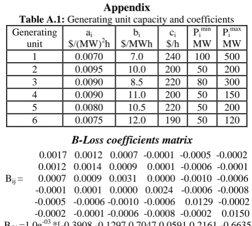
Appendix

Table A.1: Generating unit capacity and coefficients Generating

unit

ai

$/(MW)2h bi

$/MWh ci

$/h Pimin

MW Pimax

MW

1 0.0070 7.0 240 100 500

2 0.0095 10.0 200 50 200

3 0.0090 8.5 220 80 300

4 0.0090 11.0 200 50 150

5 0.0080 10.5 220 50 200

6 0.0075 12.0 190 50 120

B-Loss coefficients matrix

0.0017 0.0012 0.0007 -0.0001 -0.0005 -0.0002 0.0012 0.0014 0.0009 0.0001 -0.0006 -0.0001 Bij = 0.0007 0.0009 0.0031 0.0000 -0.0010 -0.0006

-0.0001 0.0001 0.0000 0.0024 -0.0006 -0.0008 -0.0005 -0.0006 -0.0010 -0.0006 0.0129 -0.0002 -0.0002 -0.0001 -0.0006 -0.0008 -0.0002 0.0150 BOi =1.0e-03 *[-0.3908 -0.1297 0.7047 0.0591 0.2161 -0.6635]