Scholarship & Creative Works @ Digital UNC
Scholarship & Creative Works @ Digital UNC
Dissertations Student Research
12-2019
Model Selection for Longitudinal Data With Time-Dependent
Model Selection for Longitudinal Data With Time-Dependent
Covariates Using Generalized Method of Moments
Covariates Using Generalized Method of Moments
Maryann Nishimura ShaneFollow this and additional works at: https://digscholarship.unco.edu/dissertations
Recommended Citation Recommended Citation
Shane, Maryann Nishimura, "Model Selection for Longitudinal Data With Time-Dependent Covariates Using Generalized Method of Moments" (2019). Dissertations. 643.
https://digscholarship.unco.edu/dissertations/643
This Text is brought to you for free and open access by the Student Research at Scholarship & Creative Works @ Digital UNC. It has been accepted for inclusion in Dissertations by an authorized administrator of Scholarship & Creative Works @ Digital UNC. For more information, please contact [email protected].
MARYANN NISHIMURA SHANE
Greeley, Colorado The Graduate School
MODEL SELECTION FOR LONGITUDINAL DATA WITH TIME-DEPENDENT COVARIATES USING
GENERALIZED METHOD OF MOMENTS
A Dissertation Submitted in Partial Fulfillment of the Requirements of the Degree of
Doctor of Philosophy
Maryann Nishimura Shane
College of Education and Behavioral Sciences School of Applied Statistics
and Research Methods
Entitled: Model Selection for Longitudinal Data with Time-Dependent Covariates Using Generalized Method of Moments
has been approved as meeting the requirement for the Degree of Doctor of Philosophy in College of Education and Behavioral Sciences in School of Applied Statistics and Research Methods, Program of Applied Statistics
Accepted by the Doctoral Committee
____________________________________________________ Trent Lalonde, Ph.D., Research Advisor
____________________________________________________ Han Yu, Ph.D., Committee Member
____________________________________________________ Khalil Shafie, Ph.D., Committee Member
____________________________________________________ James Kole, Ph.D., Faculty Representative
Date of Dissertation Defense __________________________________________
Accepted by the Graduate School
____________________________________________________________ Cindy Wesley, Ph.D.
Interim Associate Provost and Dean
iii
Shane, Maryann Nishimura Model Selection for Longitudinal Data with Time-Dependent Covariates Using Generalized Method of Moments. Published Doctor of
Philosophy dissertation, University of Northern Colorado, 2019.
The purpose of this dissertation was to establish measures that could be used to assess the relative fit of nested models with parameters estimated using the Generalized Method of Moments for longitudinal data with time-dependent covariates. A secondary data set collected from Filipino children was used as an example of model fitting to evaluate the quality of the assessment of fit of the Kullback-Leibler Information Criterion (KLIC) and a chi-squared statistic derived from the difference in the minimums of the quadratic forms of two candidate nested models. A simulation involving randomly-generated data sets was also used to evaluate the performance of the proposed statistics. Several variations of nested models were considered in the simulation, and the KLIC was used to compare the relative fit of these models.
Overall, the performance of the KLIC as a model selection criterion showed that it achieved good detection proportion in identifying the correct model when it was
compared to underfit models. On the contrary, it tended to favor overfit models over the correct model, and non-detection proportions were high when extraneous predictors were introduced to candidate models. Ignoring the feedback loop introduced by time-varying covariates and relying on the regular use of the Generalized Estimating Equations (GEE) for the analysis of longitudinal data could compromise model parameter consistency,
iv
with the routine use of GMM to properly account for feedback in the data is highly encouraged. The KLIC would be a helpful tool to select an appropriate model among a collection of candidate GMM models, especially when there are time-varying predictors in the data.
Keywords: model selection, fit statistic, information criterion, Generalized Method of Moments, time-dependent covariates, longitudinal data
v
This research would not have been possible without all the support I received. I dedicate this dissertation to my parents: to my mother, the most patient and caring person whose love always gets me through the hardest times; to my father, who always believed I would make something of my life and pushed me beyond my abilities. I want to thank my sister, Tina Shane, for encouraging me and making me believe in myself, and my partner in crime, Garrett Banks, for teaching me to see things through to the end.
To my friends Karen Traxler and Ben Overholt, who constantly reached out to me throughout the dissertation process, reminding me that I had someone to lean on if I ever needed help with anything: thank you both for your friendship and support. To my mentors Ron Filadelfo and Jim Jondrow: thank you for your endless support with my personal and professional development--you believed in me from Day 1, took me under your wings, and helped me become a better person through leading by example.
To my adviser, Trent Lalonde, for guiding me through a long and windy road; this research could not have happened without your support. I would also like to thank my committee members, other friends from the Department of Applied Statistics and Research Methods, my editor Judieth Hillman, and anyone else not included in this acknowledgement who have encouraged me throughout this dissertation. An astounding number of people in my life helped me in different ways and cheered for my success throughout this research. This dissertation would not have been possible without each and every one of you. Thank you all for your endless encouragement.
vi CHAPTER
I. INTRODUCTION ...1
The Purpose and Focus of the Study...4
The Need for the Study ...5
The Rationale for the Study ...6
Research Questions ...7
Overview of the Methodology ...7
Example Data Analysis ...8
The Proposed Simulation ...9
II. REVIEW OF THE LITERATURE ...12
Linear Regression ...12
Logistic Regression ...13
Longitudinal Data Models ...14
The Marginal Model ...15
The Conditional Model ...16
Time-Dependent Covariates ...17
Exogenous and Endogenous Covariate Processes ...18
Types of Time-Dependent Covariates ...19
Generalized Estimating Equations ...21
Generalized Estimating Equations and Time-Dependent Covariates ...23
Generalized Method of Moments ...25
Statistics to Assess Model Goodness-of-Fit ...29
Model Deviance ...29
Akaike’s Information Criterion ...32
Corrected Akaike’s Information Criterion ...35
Bayesian Information Criterion ...35
Quasi-Likelihood Information Criterion ...37
vii
Goodness-of-Fit of Models Estimated Using Generalized Method
of Moments ...42
Distributions of Differences in Minimands of Quadratic Forms… ...43
Hypothesis Tests for Selection of Moment Conditions ...44
Rationale for Research ...45
III. METHODOLOGY ...47
Research Questions ...48
Moment-Based Goodness-of-Fit Statistics ...48
Minimum of the Generalized Method of Moments Quadratic Form ...48
Kullback-Leibler Information Criterion ...50
Real Data ...54
Real Data: A Study on the Health of Filipino Children ...54
The Models for the Filipino Child Mortality Data...54
The Process for the Filipino Child Mortality Data ...56
Results to be Reported: The Filipino Child Mortality Data ...57
The Simulation ...58
Simulation Data ...59
Models for the Simulation Data ...61
The Process for the Simulation Data ...62
Results Reported for the Simulation Data ...63
IV. RESULTS ...66
Analysis of the Filipino Child Mortality Data ...68
Binary Response Analysis ...68
Chi-squared tests for the binary response analysis ...73
Continuous Response Analysis ...77
viii
Simulation ...85
Data Generation Process ...85
Simulation Cases ...88
Model Kullback-Leibler Information Center (KLIC) Averages ...89
Detection Proportion and Non-Detection Proportion ...93
Discussion of detection proportion ...93
Discussion of non-detection proportion ...96
Comparisons of the Simulation and Data Analysis ...98
V. CONCLUSIONS...101
Overall Findings...102
Limitations and Suggestions for Further Research ...103
Penalty for Model Complexity...103
Small-Sample Correction ...105
Performance Under Non-Binary and Non-Gaussian Responses ...106
Performance in the Presence of Type IV Time-Dependent Covariates ...107
Time-Dependent Covariate Feedback Loop Correlations ...108
Binary Time-Dependent Covariates ...109
Further Discussions ...110
Applications for Applied Research ...111
Final Remarks ...112
REFERENCES ...114
APPENDICES A. Chapter II Definitions ...123
B. Chapter IV Kullback-Leibler Information Criterion Statistics of All 31 Models for the Binary Outcome Analysis of the Filipino Child Mortality Data ...125
C. Chapter IV Kullback-Leibler Information Criterion Statistics of All 31 Models for the Continuous Outcome Analysis of the Filipino Child Mortality Data ... 128
ix
x Table
1. Kullback-Leibler Information Criterion of the Top Five
Candidate Models for the Binary Data ...70 2. The p-values of the Chi-squared Comparisons for the Binary
Data Models ...75 3. Kullback-Leibler Information Criterion of the Top Five
Candidate Models for the Continuous Data ...79 4. The p-values of the Chi-squared Comparisons for the Continuous
Data Models ...83 5. Average Kullback-Leibler Information Criterion (KLIC) of the
Models Estimated in the Simulation ...90 6. Detection and Non-Detection Proportions of the Models Estimated
in the Simulation ...94 7. Kullback-Leibler Information Criterion of All 31 Models for
the Binary Data Analysis ...126 8. Kullback-Leibler Information Criterion of All 31 Models for the
xi Figure
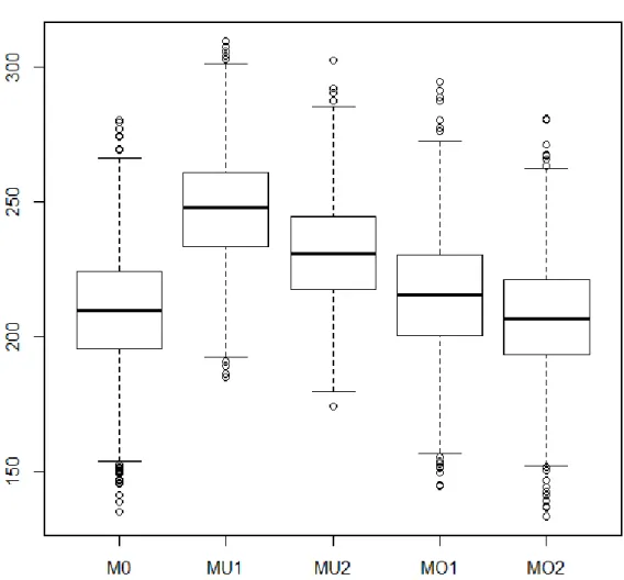
1. Kullback-Leibler Information Criterion of the 5 Models Estimated in the Simulation for the Small-Sample Binary Outcome Case
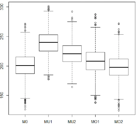
(Case 1). ...133 2. Kullback-Leibler Information Criterion of the 5 Models Estimated
in the Simulation for the Large-Sample Binary Outcome Case
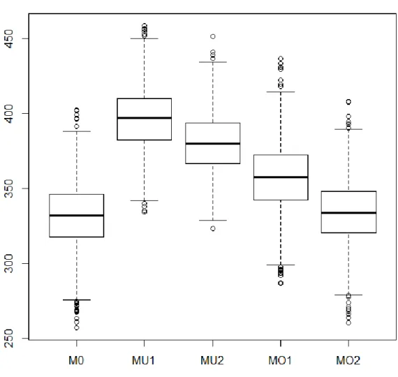
(Case 2). ...134 3. Kullback-Leibler Information Criterion of the 5 Models Estimated
in the Simulation for the Small-Sample Continuous Outcome Case
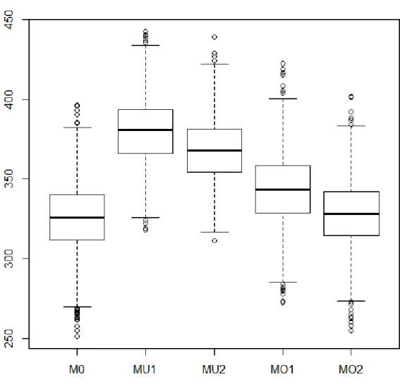
(Case 3). ...135 4. Kullback-Leibler Information Criterion of the 5 Models Estimated
in the Simulation for the Large-Sample Continuous Outcome Case
CHAPTER I INTRODUCTION
Change is an inevitable phenomenon in the natural and physical world. The concept of change has motivated human beings to study science to better understand the underlying elements that drive it. The Baltimore Longitudinal Study of Aging, conducted by the National Institute of Health, has been one of the lengthiest studies on human aging. Its objective was to understand the process of aging and the biological changes associated with aging, as well as behavioral, genetic, and external factors that impact these changes.
In the analysis of independently observed data, classical Maximum Likelihood estimation has been the most common approach. Maximum Likelihood requires knowledge of the response distribution and employs the use of the likelihood function. Maximum Likelihood estimation has oftentimes been used to estimate canonical parameters due to its property to always yield consistent estimators; moreover, if unbiased, they often have minimum variance of all unbiased estimators (McCullagh & Nelder, 1989; Mendenhall, Scheaffer, & Wackerly, 1981; Wackerly, Mendenhall, & Scheaffer, 2008).
In longitudinal studies, data are repeatedly collected from the same subjects over time. These types of studies have been frequently used in medical, educational, and environmental practices to assess the impact of a treatment or intervention over time. Compared to using the more traditional cross-sectional studies, in which observations
are made on subjects at a single point in time, longitudinal designs have the ability to detect change over time using repeated measurements of the same variables on the same subjects. Zeger and Liang (1992) support the use of longitudinal designs to analyze and better understand change over time, emphasizing their two major advantages: robustness to model selection and increased power, due to increased sample size and subjects serving as their own baseline (Zeger & Liang, 1992).
However, with more complicated designs come more complex issues involving the analysis of such data. Unlike the methods available for handling independently observed data, such as maximum likelihood, the correlation inherent in longitudinal data must be properly accounted for during analysis to prevent consequences involving modeling issues, including bias, inconsistency, and inefficiency of parameter estimates (Diggle, Heagerty, Liang, & Zeger, 2002; Fitzmaurice, 1995; Fitzmaurice, Laird, & Ware, 2011; Hedeker & Gibbons, 2006; Pepe & Anderson, 1994).
In the analysis of longitudinal data, marginal and conditional models are available. In the marginal model, the modeling of the mean and the within-subject correlation are conducted separately (Zeger & Liang, 1992), whereas the conditional model--also commonly known as the random-effects model--conditions the average response on the covariates and additional variables (Diggle et al., 2002). Marginal models focus on modeling the population average of the response, the marginal mean, whereas conditional models focus on the assumption of a level of homogeneity of repeated observations on the same subject and heterogeneity across different subjects (Diggle et al., 2002; Fitzmaurice et al., 2011). As a result, marginal models involve population-averaged conclusions, while conditional models yield subject-specific conclusions.
One of the most popular marginal methods of obtaining model parameter estimates for correlated data has been the Generalized Estimating Equations (GEE) approach (Liang & Zeger, 1986; Zeger & Liang, 1986), which employs the use of the quasi-likelihood of the response, rather than the full likelihood, as assumed in classical maximum likelihood estimation. The quasi-likelihood requires specification of only the mean and mean-variance relationship rather than the full specification of the response distribution. Similar to the popular Akaike Information Criterion, or AIC (Akaike, 1973, 1974), an information-based measure used to assess the global fit of models constructed using a likelihood-based approach, the quasi-likelihood information criterion, QIC, and its adjustment, QICu, have been used to assess the overall fit of models obtained using a quasi-likelihood approach (Pan, 2001a).
Generalized Estimating Equations (GEE) has been widely used in the handling of longitudinal data in many disciplines; however, it has encountered challenges in the presence of covariates that introduce a time-dependency to the data structure. These variables, known as time-dependent covariates (TDCs), could compromise model parameter consistency and efficiency, sometimes introduce bias when longitudinal data with TDCs are modeled using GEE, and may result in misleading inferences about the parameter estimates (Diggle et al., 2002; Fitzmaurice, 1995; Fitzmaurice et al., 2011; Pepe & Anderson, 1994). To evade some of these issues posed by GEE, the Generalized Method of Moments (GMM) has been proposed for statistical model building of
correlated data (Hansen, 1982, 2007; Lai & Small, 2007). Rather than employing the use of the quasi-likelihood of the model parameters as with GEE, the algorithm underlying
GMM uses moment conditions with zero expectation to build a quadratic form that is minimized over all parameters for model construction (Hansen, 1982).
Although GMM may improve the efficiency of model parameter estimates in the presence of TDCs (Lai & Small, 2007), one of its major disadvantages has been the lack of a universally accepted fit statistic for model selection. This research study presents two measures that could be used to compare the fit of nested models using a moment-based estimation procedure in the presence of TDCs. The focus of the first fit statistic was on an information criterion, similar in application to the popular Akaike Information Criterion (AIC; Akaike, 1973), and could be used to compare multiple nested models for the purpose of variable selection in the presence of time-dependent covariates. The second fit statistic was based on the existing quadratic form from GMM: the difference in the quadratic forms of two candidate models fit using GMM could be used to compare them inferentially using hypothesis tests.
The Purpose and Focus of the Study
The purpose of this study was to establish measures that could be used to assess the relative fit of nested models with parameters estimated using the Generalized Method of Moments for longitudinal data with time-dependent covariates. The current literature was sparse in its discussion of variable selection for correlated models involving time-dependent covariates. Model selection is important from a general modeling standpoint, and it is especially critical when different nested models require the use of different amounts and levels of resources, including time, cost, and manpower.
The focus of this study was on establishing measures to assess model fit using a moment-based method. For independently observed data, classical estimation procedures,
such as maximum likelihood, are used to construct models in which the overall goodness-of-fit or relative fit of nested models could be evaluated using statistics like the Akaike Information Criterion (AIC), model deviance, and the Bayesian Information Criterion (BIC). In using the Generalized Estimating Equations (GEE) to build models for correlated response data, the Quasi-likelihood Information Criterion (QIC) and its adjustment, QICu, could be used to assess model fit. However, when model parameters are estimated using an approach that does not involve the likelihood or quasi-likelihood functions, there was no universally accepted statistic that was used to assess model fit and compare nested models. The goal of this study was to establish such a statistic; moreover, focus was placed on an information-based measure that is analogous to the more common AIC and QIC information-based statistics. Further, a second statistic that follows a
known distribution was presented, allowing researchers to compare the fit of two specific models. The process is similar to the comparison of two candidate models using the model deviance, in which the difference of the log-likelihoods of the two models is distributed as a chi-squared statistic with degrees of freedom equal to the difference in the number of parameters of the two models.
The Need for the Study
Measures to compare nested models fit using a moment-based estimation procedure with time-dependent covariates were investigated in this study. The current literature was sparse in its discussions of model fit involving the Generalized Method of Moments and other methods that do not involve the likelihood or quasi-likelihood functions; moreover, the literature lacked discussions about the selection of
1973, 1974) has been used popularly by researchers when applying likelihood-based estimation posed with the issue of model selection. New statistics to assess GMM model fit should benefit researchers interested in moment-based estimation techniques in obtaining model parameter estimates for correlated data with time-dependent covariates.
With the era of information technology expansion and availability of bigger and more extensive data, more research has been conducted using longitudinal designs to understand change over time. However, there was very little discussion of model selection for longitudinal data involving time-dependent covariates in the current
literature, which placed a strain on the credibility of inference made by analysts who rely on the use of moment-based estimation for building correlated response models. This research was necessary in order to address the issue of model selection involving candidate nested models that are constructed using a moment-based procedure, such as the Generalized Method of Moments, when time-dependent covariates are present.
The Rationale for the Study
The statistics proposed in this research filled a gap in the current literature
pertaining to the practice of model selection for longitudinal designs with time-dependent covariates. Model selection has been important to statistical model building, and debate has continued over the traditional methods and appropriate measures for model selection. When model-based inference is at stake, the dispute over which statistic to use--even with sophisticated measures, such as the Akaike Information Criterion (AIC) and Bayes
Information Criterion (BIC)--appeared ceaseless (Buckland, Burnham, & Augustin, 1997; Burnham & Anderson, 2004; Chaurasia & Harel, 2013). Inferential results are
valid only if the selected model meets all the necessary assumptions underlying appropriate statistical modeling practices.
When multiple predictor variables are available to model the outcome of interest, and hence, several nested models are under consideration, one of the key factors that influences the decision to select a given model is the parsimony of the model relative to the amount of information lost from the data in modeling the response outcome
(Burnham & Anderson, 2004). This concern has historically been addressed with
techniques involving the use of information-based criteria for model selection (e.g., AIC, BIC, QIC, Kullback-Leibler divergence principle, etc.).
Until this research, there has been no universal statistic used to assess the fit of nested models constructed using the Generalized Method of Moments in the presence of time-dependent covariates. Measures were presented in this research study addressing the issue involving moment-based model selection.
Research Questions
The research questions answered in this study were:
Q1 How can information associated with the fit of model parameters estimated using the Generalized Method of Moments be expressed or measured?
Q2 What is the detection proportion of the model selection process of such measures in their ability to detect poor fit of underfit models?
Q3 What are the non-detection proportions of such measures in suggesting poor fit for appropriate models?
Overview of the Methodology
In order to evaluate the quality of the assessment of fit of the proposed statistics, a secondary data set collected from Filipino children to understand the relationship
between nutrition and diarrheal diseases (Bhargava, 1994; Bouis & Haddad, 1990) was used as an example of model fitting. A simulation involving randomly-generated data sets was also used to evaluate the performance of the proposed statistics. Several
variations of nested models were considered, and the proposed statistics were constructed to compare the relative fit of these models.
The simulation was not the main focus of the methods presented in this
dissertation research. Its purpose was to allow the simulation of additional data sets for the sake of evaluating the performance of the proposed statistics in assessing model fit.
Example Data Analysis
Researchers of the International Food Policy Research Institute (IFPRI) collected data from Filipino children, aged 1-10 years, from the island of Mindanao between 1984 and 1985 to study the relationship between nutrition and health (Bhargava, 1994; Bouis & Haddad, 1990). Age, gender, height, weight, food consumed, illnesses suffered, the duration of illnesses, as well as descriptive information about the parents, were collected from 448 households using 4 surveys each 4 months apart. These primary data were used as secondary data in this research study. As correlation in nutritional quality was
expected from siblings or from children within the same household, data from only the youngest child were kept. Additionally, observations with missing values were omitted, resulting in balanced longitudinal data containing information from 370 children at 3 time points (Bhargava, 1994; Bouis & Haddad, 1990).
From these longitudinal data, five variables were selected as potential predictors, as well as a binary response, to estimate a logistic regression model. In addition, a variation of the response defined by a transformation of the illness-related variables was
used as a continuous response variable for a multiple linear regression model. The information-based measure to assess fit was obtained and compared for all possible models that could be constructed from different combinations of five predictors. This measure was used to determine the most “ideal” candidate model to predict the probability of illness for the logistic regression model and to predict morbidity for the multiple linear regression models. Then, these models were compared to those obtained in the study by Lai and Small (2007).
Using the models that yielded the five smallest values of the information criterion, the statistic based on the difference in the minimums of two GMM quadratic forms from pairs of candidate models was obtained to assess significant departure of the candidate model from a model with adequate fit. The model selected as most ideal using the information-based measure of fit was compared to the remaining four models, for a total of four pairwise comparisons.
The Proposed Simulation
As only one set of models could be constructed from the real data, only one set of statistics could be obtained to assess the quality of fit of the candidate models for each of the two proposed statistics. Therefore, there was a need for a simulation to generate additional data sets for the sake of evaluating the performance of the proposed information criterion. A simulation was used to obtain more estimates of the two proposed statistics--the information-based statistic and the measure based on the minimums of two GMM quadratic forms--to assess their performance in analyzing fit. The software environment R version 3.1.0 was used to produce these data and perform all necessary analysis.
For the data simulation, both binary and continuous correlated responses were randomly generated to estimate logistic regression and multiple linear regression models. Continuous predictors, including time-dependent covariates (TDCs) of Types II and III, were also randomly generated, to keep the data structure consistent with that of the Filipino child study. A true model was defined as one that included three predictors, two of which were TDCs of Types II and III. The third predictor in the true model was a Type I TDC, to simplify the data analysis procedure. Two unnecessary predictors that were TDCs of Types II and III were also randomly generated. With attention paid to the
performance of the proposed fit statistics when TDCs of Types II and III were improperly included or omitted, two overfit and two underfit models were examined in comparison to the true model. One of the overfit models included an additional unnecessary Type II TDC, and the other overfit model included an unnecessary Type III TDC. These models were used to assess the non-detection proportions of the proposed fit statistics, or the proportion of times in the simulation that an incorrect predictor was not detected by the KLIC. Similarly, one of the underfit models omitted a necessary Type II TDC, and the second underfit model omitted a necessary Type III TDC, and these models were used to evaluate the detection proportion of the proposed statistics in assessing adequate model fit, or the proportion of times that an incorrect predictor was correctly detected by the KLIC.
In the simulation, 2000 data sets (Lai & Small, 2007) were randomly generated for both small-sample and large-sample situations, as well as for the binary and
continuous response cases. Following the simulation study by Lai and Small (2007), the small sample included a total of 500 observations, and the large sample included a total
of 2,500 observations. For these data to be balanced in longitudinal structure with T = 5 repeated observations per subject, the small sample included I = 100 subjects, and the large sample included I = 500 subjects. A discussion of the issues presented by the use of unbalanced data was included in the Limitations section in Chapter V. For each of the sample size conditions, the proposed fit statistics were obtained for each replicate.
The organization of this research follows: Chapter II provides an extensive review of the current literature involving the subject matter, and Chapter III delineates the
methods used in evaluating the performance of the proposed statistics in assessing model fit. The analysis of the real data and the details of the simulation are described in Chapter IV, and a discussion of the results and conclusions that could be drawn from this research study are included in Chapter V.
CHAPTER II
REVIEW OF THE LITERATURE
In the literature review, various fit statistics were discussed for different
estimation methods of parameters for longitudinal data models, with a focus on logistic regression models. For classical maximum likelihood estimation of independent data, the most common statistics used in assessing model fit was the deviance, the Akaike
Information Criterion (AIC), and the Bayes Information Criterion (BIC), also known as the Schwarz Information Criterion (Cavanaugh & Neath, 1999). When using Generalized Estimating Equations (GEE) to estimate model parameters for correlated data,
modifications of the AIC, known as the quasi-likelihood information criterion (QIC) and its adjustment, QICu, were used. There has been no popular method yet in assessing goodness-of-fit (GOF) for models derived from the Generalized Method of Moments (GMM) process. A review of the literature highlighted the need for such a GOF statistic, and details are given in the subsequent chapter.
Linear Regression
A linear regression model assumes the equation:
𝑌𝑖𝑡 = 𝛽0+ 𝛽1𝑥𝑖𝑡1 + 𝛽2𝑥𝑖𝑡2+. . . +𝛽𝑘𝑥𝑖𝑡𝑘+ 𝜀𝑖𝑡,
where i = 1,..., N denotes subjects; t = 1,..., T denotes observation time; the mean response Yit = g−1(0+1xit1 +2xit2 +...+k xitk)for subject i is a function of the
parameters (β0, β1,..., βk); g is the identity-link function;xitjis the j
time t for subject i for j =(1,…, k), and ɛit is random error. For independent data, the i
index is maintained to identify subjects, but there is no time index (t), denoting different observation times.
Logistic Regression
The primary focus was on a logistic regression model:
k it k it it it it it p x x x p p it = + + + + − = ... 1 ln ) ( log 2 1 2 1 0 , (1)
where i = 1,..., N denotes subjects; t = 1,..., T denotes observation time; the mean
response pit = ( ... ) 2 1 2 1 0 1 k it k it it x x x
g− + + + + for subject i is a function of the
parameters (β0, β1,..., βk); g is the logit-link function; and xitjis the jth covariate value at
time t for subject i for j =(1,…, k).
For independent data, the t index in Equation (1), denoting different observation times, was omitted; the i index was maintained to identify subjects. In matrix notation, the logistic regression model in Equation (1) could be written as:
( ) iT
g pit =X , (2)
where g is the logit-link function; pi is the vector of mean responses for subject i, which is equivalent to the probability of success for binary responses; Xi =
it it it
Tk x x x , ,..., , 1 2 1 is
the vector of covariates for subject i; and β =
0,1,...,k
Tis the vector of parameters. Additionally, a binomial response distribution was assumed:(
it)
it Bin n p
Y = ,
As with ordinary regression models, logistic regression was used to model the mean response--in this case, the probability of success. The conditional mean, E Y
it|Xi
,was modeled, rather than modeling the expected response, E
Yit (Hosmer & Lemeshow,2000):
it|
0 1 it1 2 it2 ... k itkE Y Xi = + x + x + + x . (3)
A link function was used to link pit, the probability of success, with the
parameters of the model. In the case of a logistic regression model, the logit-link
function, logit(pit) = − it it p p 1
ln , is commonly used to link pit with the model
parameters (Hosmer & Lemeshow, 2000; Hosmer, Lemeshow, & Sturdivant, 2013).
Longitudinal Data Models
Longitudinal data, by definition, are data that are collected from the same individuals, or objects, multiple times using the same measure(s). Examples of longitudinal studies included the National Health and Nutrition Examination Survey (NHANES) and the National Education Longitudinal Study (NELS). The NHANES is an annual survey research study conducted by the National Center for Health Statistics (NCHS) to assess the health and nutritional status of Americans between the ages of 1 and 74. Fifteen participants have been followed annually since 1999 to maintain repeated observations of the same subjects, and the longitudinal database focuses on repeated measurements from these 15 individuals. National Education Longitudinal Study (NELS) is an education survey conducted by the National Center for Education Statistics (NCES) to assess the achievement and learning of eighth graders. A sample of the original group of eighth graders was followed four times at irregular intervals since 1988, and the main focus of these data was on the longitudinal information obtained from this subgroup.
In the handling of longitudinal data, the assumption of independently and identically distributed (i.i.d.) observations is not maintained due to the correlation inherent in repeated observations of subjects. As a result, an estimation method that accounts for correlated data, a process that could detect changes in the mean response over time, must be employed. To do this, two types of models were commonly used in the existing literature: the marginal model and the conditional model. For the sake of this research, a balanced design was assumed. A balanced design is one in which the
responses of every subject are observed an equal number of times at equal intervals apart. A logistic regression model was still considered, as described at the beginning of this chapter.
The Marginal Model
In the marginal model, the mean and the within-subject correlation are modeled separately (Zeger & Liang, 1992). The marginal mean is the average response,
conditioned on the covariates of subject i (Diggle et al., 2002), as represented by
Equation (3). The marginal model links the marginal mean to covariates via the relation in Equation (2) using a known link function, g (Diggle et al., 2002; Fitzmaurice, 1995; Fitzmaurice et al., 2011; Hedeker & Gibbons, 2006; Zeger & Liang, 1992). As the focus of this research was in dealing with binary responses, g was the logit-link function.
In the marginal model, the focus is on modeling the within-subject correlation separately from the marginal regression of the response on the predictor variables (Diggle et al., 2002). In other words, the primary focus of marginal models is to model the
systematic variation associated with the mean separately from the random variation that arises as a result of the repeated observations (Fitzmaurice et al., 2011). Assumptions are
made about the mean response, E
Yi , as well as the covariance of the responses,( )
Var Yi , and estimates are obtained for both the vector of parameters, β, and the vector
of within-subject correlations, α (Diggle et al., 2002). Additionally, the marginal variance is a function of the marginal mean such that:
( ) ( )
it itVar Y = v p φ,
where v is a known function and φ is the over-dispersion parameter which accounts for the variation in Yit not explained by v(pit). The covariance between Yit and Yis, for a time
point s ≠ t, is a function of the marginal means and possibly additional parameters α,
(
is it) (
is it)
Cov Y ,Y = c p , p ;α ,
where c is a known function and the values of α are the parameters in the correlation or covariance matrix. In a marginal model, the correlation between two repeated
observations from the same subject is assumed to depend only on the time between the two measurements, represented by α (Zeger & Liang, 1986).
Marginal models yield population-averaged conclusions (Zeger, Liang, & Albert, 1988). For logistic regression scenarios, the results of population-averaged models involve comparisons between two populations, or a reference group and a compared group, using odds ratios. Comparisons between the populations are expressed as the average change in the expected transformed response for a unit change in the value of a predictor of interest, holding all other predictors constant (Hosmer & Lemeshow, 2000; Hosmer et al., 2013; Menard, 2002).
The Conditional Model
In contrast to the marginal mean, the conditional mean is the average response conditioned on the covariates Xi and additional variables Bi:
it
0 1 it1 2 it2 k itkE Y |X Bi, i = β + β x + β x + ...+ β x +Bi.
The conditional model links the conditional mean to both the covariates Xi and the additional variables Bi using the conditional regression parameters β and additional parameters γ (Diggle et al., 2002; Fitzmaurice et al., 2011; Hedeker & Gibbons, 2006):
( )
T= T +γ
i i i
g p X β B .
This is akin to a random-effects model, in which the correlation among responses for a given subject is assumed to arise from natural heterogeneity in regression
coefficients across different individuals (Zeger & Liang, 1986, 1992). The additional variables, Bi, are assumed to contain information about this homogeneity within and heterogeneity across subjects: the conditional model assumes that there are unobserved factors underlying the homogeneity of responses within a subject, thus inducing
correlation within repeated observations on the same subjects, but that those factors vary across different individuals (Diggle et al., 2002).
Conclusions drawn from conditional models differ from the population-averaged conclusions made from marginal models. Conditional models are associated with subject-specific conclusions (Zeger et al., 1988). Parameter coefficients of conditional models are interpreted as the average change in the expected transformed response associated with a change in the predictor variable for a specific subject, holding all other predictors
constant. However, conditional models were not the primary focus of this research; the marginal model was used in this study.
Time-Dependent Covariates
Time-dependent covariates (TDCs) are predictors whose values change over time, within a group, subject, or cluster. Weight, height, age, and study cohort are all variables
that could be TDCs. Any covariate that changes in value over time or changes over the course of repeated observations could be a time-dependent covariate (Diggle et al., 2002; Lai & Small, 2007; Neuhaus & Kalbfleisch, 1998). The age of a participant in a
longitudinal study to assess hypertension is an example of a time-dependent covariate because the participant’s age would increase over time. Annual glacial coverage in an ongoing study to assess causation and impact of global climate change, as well as the amount of chemical substance present in the half-life of a radioactive material, are also examples of time-dependent covariates. These special types of covariates introduce correlation among variables over time, and this correlation must be accounted for when constructing models for longitudinal data. Failure to account for this correlation when constructing models may result in loss of efficiency and increase the possibility of biased parameter estimates (Fitzmaurice, 1995; Lai & Small, 2007; Pepe & Anderson, 1994).
The importance of accounting for the temporal nature of time-dependent
covariates and the subsequent impact on the analysis of longitudinal data is highlighted by the difference between endogenous and exogenous covariate processes. The following section differentiates these processes and provides an explanation in the context of a data feedback loop.
Exogenous and Endogenous Covariate Processes
Diggle et al. (2002) defined an exogenous process as one in which the covariate at a given time, t, was conditionally independent of response measurements prior to that time. In other words, a covariate process is exogenous if there is no response feedback to the covariate. Exogeneity implies that the mean response for subject i at time t,
conditioned on all covariate values (at other times) xi1, xi2,..., xiT, only depends on the
covariates prior to time t:
Yit|xi1,xi2,...,xit
=E
Yit|xi1,xi2,...,xi,t−1
E .
Exogeneity also implies that the response for subject i at time t is conditionally independent of all future covariates, given both the past response and covariate values (Diggle et al., 2002). Any variable external to a study is an exogenous covariate. In the previously mentioned example of a study in which age was examined to assess a participant’s risk of hypertension, weather was a possible exogenous variable.
On the other hand, an endogenous process is one in which feedback may be present: the response for subject i at time t could be associated with the covariate value at future time points. Diggle et al. (2002) described an endogenous covariate as both a predictor of the outcome of interest, as well as a measure that was predicted by the outcome at an earlier time. Hence, an endogenous process could involve a complex feedback loop in which the covariate influences the response, and the response influences the covariate (Diggle et al., 2002; Zeger & Liang, 1991).
Types of Time-Dependent Covariates
Recent literature has defined four types of time-dependent covariates (TDCs), and distinctions were made based on the nature of their feedback (Lai & Small, 2007;
Lalonde, Wilson, & Yin, 2014). Covariate types were defined as follows. Consider a model defined as:
(
)
= g T
i i
p X β ,
where pi is the mean response for subject i, g is a known link function, Xi is the vector of covariates for subject i, and β is the vector of model parameters. The four types of TDCs
were defined by the combinations of s and t that maintain the equality in the expression (Lai & Small, 2007; Lalonde et al., 2014):
( )
0 ( 0)
=0 − it it j is y p p E , (4)where pis is the mean response for subject i at time s, βj is the jth covariate, yit is the
response for subject i at time t, pit is the mean response for subject i at time t, β0 is the
vector of true parameters, and s and t are different observation times, where s (1,…,T) and t (1,…,T).
A Type I time-dependent covariate satisfies the zero expectation of Equation (4) for all values of s and t, s (1, …, T) and t (1, …, T). Type II TDCs satisfy the zero expectation of Equation (4) for all combinations of s and t such that s ≥ t. Type III TDCs satisfy Equation (4) for s = t. Lastly, a Type IV TDC satisfies the zero expectation of Equation (4) for all combinations of s and t such that s ≤ t. Association between the derivative term at time s and the residual term at time t violates the equality in Equation (4), resulting in a non-zero expectation. In order for the zero expectation to be held, the assumption:
it
it
E y |Xit = E y |Xi1,...,XiT ,
must be maintained for all s and t, for s (1, …, T) and t (1, …, T). When time-varying covariates are present in the data, this assumption is oftentimes violated. Details are discussed in the Generalized Estimating Equations and Time-Dependent Covariates section.
A Type I TDC involves no feedback; the current covariate affects only the current response. A covariate that affects both the current and future responses is a Type II TDC.
The nature of the feedback involved in the presence of Type III TDCs creates a complex feedback loop in which the current response affects the covariate at some future time, and the current covariate affects the response at some future time. Type IV TDCs are often thought of as the “opposite” of Type II TDCs; when Type IV TDCs are present, the current response is associated with the current covariate, and the current response could also be associated with the covariate at some future time (Lai & Small, 2007; Lalonde et al., 2014).
Due to the nature of the time-dependence imposed by TDCs on the data structure, the analysis of longitudinal data in the presence of TDCs could become challenging very quickly (Diggle et al., 2002; Neuhaus & Kalbfleisch, 1998). Moreover, depending on the method of analysis chosen, algorithm non-convergence of parameter estimation may be an additional hurdle in the process of obtaining model parameter estimates (Kleiber & Zeileis, 2008).
Generalized Estimating Equations
One of the most popular techniques for marginal model parameter estimation in the analysis of correlated data has been the Generalized Estimating Equations (GEE) approach (Liang & Zeger, 1986; Zeger & Liang, 1986). The GEE method uses an assumed working correlation structure for the data under investigation. A working correlation structure (e.g., compound symmetry, order-m auto-regressive, exponential, etc.) that likely characterizes the nature of the correlation prevalent among repeated response measurements for each subject is proposed. Generalized Estimating Equations (GEE) uses estimating equations of the form:
( )
1( )(
)
1 cov 0 N i S − = = − =
i i i i p y y p ,where pi is the vector of mean responses for subject i, β is the vector of parameters, and yi is the vector of observed responses for subject i, for a total of N subjects (Liang & Zeger, 1986; Zeger & Liang, 1986). The covariance term, cov(yi), is calculated using the
working correlation structure.
An advantage of using Generalized Estimating Equations in the analysis of longitudinal data could be that, regardless of whether or not the “correct” working correlation structure is selected, GEE parameter estimates are consistent (Diggle et al., 2002; Fitzmaurice, 1995; Liang & Zeger, 1986; Neuhaus & Kalbfleisch, 1998).
Additionally, the GEE approach does not require full specification of the response distribution. It only requires information involving the mean and mean-variance relationship of the response, hence only assuming a quasi-likelihood instead of the full likelihood (Liang & Zeger, 1986; Zeger & Liang, 1986).
The covariance matrix used in the GEE process depends on the selection of the working correlation structure, Ri(α) (Fitzmaurice, 1995; Hin & Wang, 2009; Liang, Zeger, & Qaqish, 1992; Zeger & Liang, 1986), where the parameters α are part of the structure of Ri. If the compound symmetry structure is assumed, then the correlation αs,t
among pairs of time points s and t is equivalent regardless of the combination of times; hence, only one value (i.e., α) need be estimated. The estimating equations for the vector
α have the form:
( )(
)
0 cov ) ( 1 1 = − = − =
i i i N i i w w S ,where α is the vector of parameters from the specified working correlation structure, wi is the vector of covariances for pairs of responses at different combinations of time points s
and t (s, tT), and ηi is the vector of expected covariances, or ηi = E[wi] (Liang et al., 1992).
In order to obtain the GEE estimators, the estimating equations would iteratively be solved for the regression coefficients, β, and the correlation parameters, α. Given an estimate of the working correlation structure,Ri
( )
ˆ , iteratively reweighted least squares is applied to obtain an updated ˆ (McCullagh & Nelder, 1983). Once ˆ is obtained, a second set of estimating equations is used to obtain consistent estimates of α. This process is repeated until convergence is achieved (Liang et al., 1992).Generalized Estimating Equations and Time-Dependent Covariates
Oftentimes in longitudinal designs, time-dependent covariates are present in the data structure. The Generalized Estimating Equations method was often applied to obtain parameter estimates in the presence of time-dependent covariates. Pepe and Anderson (1994) and Fitzmaurice (1995) advised that, when TDCs were present in the data, a critical assumption behind the Generalized Estimating Equations process should be confirmed when using it for parameter estimation. Specifically, GEE relies on the assumption of the marginal expectation,
Y x
E Y x s T
E it| it = it| is, =1,..., , (5)
where Yit is the response for subject i at time t (t = 1, …, T), xit is the covariate value for
subject i at time t, and xis is the covariate value for subject i at time s (s = 1, …, T). This
assumption states that for subject i, the expected response at time t, given the covariate value at that same time, should be equal to the expected response at time t, given the covariate value at all times (Fitzmaurice, 1995; Pepe & Anderson, 1994). In other words,
for a given subject, the covariate values at other times would not affect the conditional expected response at time t.
The marginal expectation represented by Equation (5) was an assumption that was necessary for the zero expectation of the Generalized Estimating Equations. As an
alternative to checking this assumption, using a diagonal working correlation--such as the independent working correlation structure--ensures that the expectation of the generalized estimating equations is 0 (Diggle et al., 2002; Fitzmaurice, 1995; Pepe & Anderson, 1994):
1( )(
)
1 ( ) cov N i E S E − = = − =
0 i i i i p y y p .Evaluating the expectation is equivalent to integrating over all ℝT,
( )(
)
1 1 1 cov T N i d N − = − =
i 0 i i i i p y y p y .The only random components of S(β) are the response values; the derivative and covariance matrices are composed of fixed values, so they could be brought outside of the integration process, provided that the derivative of the systematic component is independent of the raw residuals:
( )(
)
0 cov 1 1 1 = −
= − i N i i i i i y y p dy p N T .Using a diagonal covariance matrix such as the independent structure, IT, ensures that the derivative terms and residual terms at only the same times are matched, satisfying the assumption of independence for a correctly specified model (Diggle et al., 2002; Fitzmaurice, 1995; Pepe & Anderson, 1994). The use of a diagonal covariance matrix
maintains the zero expectation, and the assumption in Equation (5) is no longer relevant, and the integral simplifies to a scalar:
(
)
0 1 1 1 = −
= = it T t it it j it N i dy p y p N T .However, if the covariance matrix is not diagonal, derivative and residual terms from various time points are matched, and the expectation may not equal 0 (Diggle et al., 2002; Pepe & Anderson, 1994).
Oftentimes when time-dependent covariates are present, the equality in Equation (5) does not hold (Fitzmaurice, 1995; Pepe & Anderson, 1994). Moreover, Fitzmaurice (1995) warned that the efficiency of an Independent GEE estimator that was associated with TDCs depended on the strength of the correlation between the responses; efficiency decreased drastically as the ignored correlation among responses increased. Although the use of the independent working correlation structure was recommended, in general, when time-dependent covariates were present, assuming independence between responses for subject i at different times could result in decreased efficiency of parameter estimates associated with that covariate (Fitzmaurice, 1995). In other words, the more significant the information being ignored, the greater the loss in efficiency.
Generalized Method of Moments
An alternate approach that could be taken in estimating parameters for marginal models of correlated data was to implement Generalized Method of Moments estimation (Hansen, 2007). The Generalized Method of Moments (GMM), like the Generalized Estimating Equations, is a method that accounts for correlation inherent in the data due to repeated measurements taken on the same subjects. Unlike GEE, GMM relies on the use
of moment conditions, expressions with zero expectation, rather than on the derivation of the likelihood or quasi-likelihood functions.
The process behind GMM involves minimizing a quadratic form, QN, over the
parameters β (Hansen, 1982, 2007; Lai & Small, 2007):
( )
( )
T( )
N
Q =GN W GN N , (6)
where WN is a weight matrix. The vector GN in Equation (6) is the average of moment conditions for all N subjects:
(
)
1 1 , , N i i g N = =
0 N i G Y X β ,where Yi is the vector of responses for subject i, Xi is the vector of covariates for subject
i, β0 is the vector of true parameters, and g(Yi, Xi, β0) would be denoted gi(Yi, Xi) for short.
When time-dependent covariates are present, the vector gi(Yi, Xi) is composed of only the moment conditions that are considered “valid” for subject i, defined by Lai and Small (2007) as satisfying the expression:
E [gi(Yi, Xi)] = 0 .
Lai and Small (2007) proposed using moment conditions that were products of derivative and residual terms at different times:
(
it it)
j is i y p p g − = ,where pis is the mean response for subject i at time s (s = 1, ..., T), yit is the response value
for subject i at time t (t = 1, ..., T), pit is the mean response for subject i at time t, βj is the
jth covariate, i (i = 1, ..., N) denotes the subject, and gi denotes the vector of valid moment conditions for subject i. Moment conditions are selected based on the type of
time-dependent covariates included in an analysis. For continuous data, pis and pit are replaced
by the average response at time s and at time t, µis and µit, respectively. Further, it has
been shown that the optimal choice for the weight matrix, WN, in Equation (6) is to use the inverse of the covariance matrix of the moment conditions (Hansen, 1982):
( )
1 1 ˆ − Cov− = = N N i W V g .There have been several variations of the Generalized Method of Moments procedure, such as the Continuously Updating GMM, 2-Step GMM, and Iterative GMM (Chaussé, 2010; Hall, 2005; Hansen, 1982, 2007; Nielsen, 2005; Zivot, 2015). The difference in these types is determined by the choice of the weight matrix applied in the quadratic form that is minimized to obtain parameter estimates, and hence, the standard errors vary slightly. The quadratic forms minimized in the process behind the two most commonly used GMM types, Continuously Updating GMM (CUGMM) and 2-Step GMM (2SGMM), are:
( )
1( ) ( )
: T CUGMM QF GN VN− GN ( )
1( )
( )
2 : ˆ ˆ T SGMM QF GN VN− GN .To obtain a 2SGMM estimator, an arbitrary initial weight matrix is selected, such as the identity matrix. This weight matrix is used to obtain the initial inefficient GMM estimator, ˆinitial. Using this inefficient estimator, an optimal weight matrix could be found, and this optimal weight matrix is used to obtain an efficient GMM estimator,
ˆ
efficient
(Hansen, 1982; Mátyás, 1999; Nielsen, 2005). Due to its dependence on the choice of the initial weight matrix, the 2SGMM estimator is not unique. Continuously Updating GMM (CUGMM) estimators, on the other hand, do not depend on the initial
weight matrix; rather, the weight matrix depends on the parameters (Nielsen, 2005; Zivot, 2015). The CUGMM estimation process simultaneously estimates the parameters, β, and the weight matrix as a function of the parameters, W(β) (Mátyás, 1999; Zivot, 2015).
Hence, with 2SGMM, VˆN−1
( )
ˆ is fixed during the minimization of the quadratic form; whereas with CUGMM, the weighting matrix changes when β is changed in theminimization process (Chaussé, 2010; Mátyás, 1999; Nielsen, 2005; Zivot, 2015). In obtaining the covariance matrix used to construct the quadratic form, QN, for
obtaining GMM parameter estimates, Hansen (2007) additionally suggested the use of an iterative procedure in which an initial consistent GEE estimator % is used to obtain cov{g(Yi, xit, β0)}-1, then estimating βGMM using
1 ˆ −
N
V , yielding an estimator that is as
asymptotically efficient as the traditional 2-Step GMM estimator and has consistent asymptotic variance (Hansen, 2007; Lai & Small, 2007), given by:
(
)
(
) (
)
1(
)
1 1 1 1 , , , , 1 1 1 , , , , T N N T N it it i it i it i i i x x x g Y x N N N − − = = =
% % i i g Y g Y g Y where (
i,xit,)
g Y is evaluated at β = ˆGMM (Hansen, 2007). This research focused on
the use of the 2-Step GMM.
In comparison to using the Independent GEE approach, the use of GMM estimation improved efficiency when time-dependent covariates were present. Results from the simulation study by Lai and Small (2007) showed that GMM estimators were more efficient than Independent GEE estimators when time-dependent covariates of types I or II were involved, and they were equally as efficient as Independent GEE estimators when a TDC of Type III was present. Moreover, in general, GMM estimators were
equally as efficient as GEE estimators when the working correlation structure was correctly specified, and they were asymptotically more efficient than GEE estimators when the working correlation structure was misspecified (Lai & Small, 2007). For these reasons, GMM estimation was a superior method when compared to Independent GEE when estimating parameters of a longitudinal study involving time-dependent covariates.
Statistics to Assess Model Goodness-of-Fit
For classical maximum likelihood estimation of independently observed data, some common statistics used in assessing model fit include the model deviance (Agresti, 1990; Dobson & Barnett, 2008; Pregibon, 1981), Akaike’s Information Criterion, or AIC (Akaike, 1973, 1974), and Schwarz’s Bayesian Information Criterion, or BIC (Schwarz, 1978). When using the Generalized Estimating Equations to estimate model parameters for correlated data, a modification of the AIC, known as the quasi-likelihood information criterion, or QIC (Pan, 2001a), and its adjustment, QICu, are used.
Model Deviance
To assess the fit of any generalized linear model, statisticians commonly use a goodness-of-fit measure known as the model deviance. Deviance gives a measure of the deviation of a specific model from the data. The likelihood evaluated using the data yields a model of “perfect fit” (Agresti, 1990). For discrete predictors, the model has as many parameters as observations. Deviance is a useful tool in assessing the goodness-of-fit of a model in that it could be used to compare a specific model to the full data, and it could also be used to compare two nested models.
When comparing a specific model to the data, deviance is given by:
(
; ˆ)
2( ) (
; ˆ;)
where L
(
ˆ ;y)
is the maximum value of the log-likelihood under the given model, and L(y; y) is the maximum of the log-likelihood under the full data (Agresti, 1990). In other words, the deviance of a specific model, compared to the saturated model (i.e., the full data), is the difference in likelihoods under these two models. Because the log-likelihood is used, deviance could also be thought of as the log of the ratio of the likelihoods under the two models.It is also known that:
(
; ˆ)
D y ~ χ2 (N – k) ,
where N denotes the number of observations in the data and k denotes the number of parameters in the specified model (Agresti, 1990). The sampling distribution for the deviance results directly from the difference in log-likelihoods of two candidate models (Dobson & Barnett, 2008). For example, if ˆ is the maximum likelihood estimator for the parameters β0 of a “true” model M0, the difference in log-likelihoods of ˆ and β0 could be written approximately:
(
)
( )
ˆ 1(
ˆ) ( ) (
ˆ ˆ)
; ;
2
T
l β y0 −l y = − β0− β0− ,
where ℑ is Fisher’s information matrix.
For linear models, Fisher’s information matrix is equivalent to:
2
1 T
= X X
,
For nonlinear models, Fisher’s information matrix is equivalent to: 2 l = β βi j .
Then, the following statistic:
( )
ˆ(
)
(
ˆ) ( ) (
ˆ ˆ)
2l ;y −l β y0; = β0− T β0−
is distributed as a chi-squared distribution χ2(p – k) with p = number of parameters in the
“true” model, and k = number of parameters in the candidate model.
When comparing two nested models, models M1 and M2, where M2 is nested
within M1, the deviance is given by:
(
; ˆ)
(
; ˆ)
2(
ˆ ;)
(
ˆ ;)
D y μ2 −D y 1 = L 2 y − L 1 y ~ χ2
(p1 – p2) ,
where p1 - p2 denotes the difference in the number of parameters in the two models
(Agresti, 1990). Since model M2 is nested within M1, the parameters of the vector β2 for
M2, is a subset of the parameter vector β1 for M1.
No matter the models being compared--whether it be two nested models or a specific model compared to the saturated model--deviance is calculated as the difference in the log-likelihood of two models, or the likelihood ratio of two models (Agresti, 1990). It is the information not explained by the smaller model. It is similar to the Mean Squared Error (MSE) of a regression model, which gives an estimate of unexplained random error in the model. Moreover, model deviance is always distributed as a chi-squared
distribution with degrees of freedom equal to the difference in the number of model parameters of the two models being compared.
Because the distribution of the model deviance is always known, hypothesis tests could be formed to assess model fit. The null hypothesis assumes the model fit for the
smaller model to be “sufficient.” Smaller values of the chi-squared statistic suggest less deviation of overall goodness-of-fit of the candidate model from the “null” model (i.e., the data). In general, a small value of the deviance suggests that the smaller model is just as informative as the “null” model. The alternative, evidence to reject the null hypothesis, indicated by a large chi-squared test statistic, assumes poor fit for the smaller model.
Akaike’s Information Criterion
To assess the fit of models derived using maximum likelihood estimation, researchers oftentimes rely on an information-based fit statistic known as Akaike’s Information Criterion (AIC), proposed by Akaike (1973). Akaike’s Information Criterion assumes no distribution; rather, it is a single value that is used descriptively to represent the amount of information lost from fitting a specific model to the data. It does not require the comparison of two nested models but rather compares a model to the actual data (Akaike, 1973).
Due to the asymp