Research Article
Pixel Intensity Clustering Algorithm for
Multilevel Image Segmentation
Oludayo O. Olugbara, Emmanuel Adetiba, and Stanley A. Oyewole
ICT and Society Research Group, Durban University of Technology, P.O. Box 1334, Durban 4000, South Africa Correspondence should be addressed to Oludayo O. Olugbara; [email protected]
Received 20 May 2015; Accepted 12 July 2015 Academic Editor: Mar´ıa I. Herreros
Copyright © 2015 Oludayo O. Olugbara et al. This is an open access article distributed under the Creative Commons Attribution License, which permits unrestricted use, distribution, and reproduction in any medium, provided the original work is properly cited.
Image segmentation is an important problem that has received significant attention in the literature. Over the last few decades, a lot of algorithms were developed to solve image segmentation problem; prominent amongst these are the thresholding algorithms. However, the computational time complexity of thresholding exponentially increases with increasing number of desired thresholds. A wealth of alternative algorithms, notably those based on particle swarm optimization and evolutionary metaheuristics, were proposed to tackle the intrinsic challenges of thresholding. In codicil, clustering based algorithms were developed as multidimensional extensions of thresholding. While these algorithms have demonstrated successful results for fewer thresholds, their computational costs for a large number of thresholds are still a limiting factor. We propose a new clustering algorithm based on linear partitioning of the pixel intensity set and between-cluster variance criterion function for multilevel image segmentation. The results of testing the proposed algorithm on real images from Berkeley Segmentation Dataset and Benchmark show that the algorithm is comparable with state-of-the-art multilevel segmentation algorithms and consistently produces high quality results. The attractive properties of the algorithm are its simplicity, generalization to a large number of clusters, and computational cost effectiveness.
1. Introduction
Image segmentation remains an important problem in the fields of digital image processing, pattern analysis, image understanding, and computer vision. It is the process of subdivision of an image into homogeneous and disjoint sets sharing similar properties such as intensity, color, and contour [1]. Applications of image segmentation cut across disciplines as diverse as pattern recognition, image compres-sion, content-based image retrieval, image processing, micro-scopic imaging, automatic image analysis, image and video understanding, video security, computer-aided surgery, auto-mated medical diagnosis, human-machine interface, mov-ing object trackmov-ing, image enhancement, biometric access control, computer vision, deoxyribonucleic acid sequencing, automatic vehicle recognition, optical character recognition, remote sensing, land cover classification, and machine learn-ing [2–10]. Image segmentation is not a trivial problem because the majority of images are affected by factors such
as noise content, occlusion, weak object boundary, inho-mogeneous object region, weak contrast, nonuniformity of
illumination, and reflectance [4, 11]. Different algorithms
have been proposed over the years for image segmentation and two important properties commonly employed to cat-egorize various segmentation algorithms are homogeneity and discontinuity of pixel properties. Edge-based methods are based on pixel discontinuity properties and they segment images by detecting pixels with rapid transition in intensities
between regions [12,13]. The image segmentation methods
based on the property of homogeneity include thresholding, clustering, and region growing as well as region splitting and
merging [14,15]. These methods segment images based on
the predefined objective functions and characteristics such as texture, shape, color, intensity, and other domain specific
features [11,16].
Image thresholding is very popular because it offers intrinsic benefits such as compact storage space, fast execu-tion speed, simplicity, low computaexecu-tional cost, and real-time
Volume 2015, Article ID 649802, 19 pages http://dx.doi.org/10.1155/2015/649802
applicability [17,18]. Thresholding attempts to identify and extract an object from its background on the basis of the distribution of gray levels or texture in the image object [19]. The prime objective of gray level image thresholding is to
divide a gray level image into a𝐾-number of predetermined
partitions or clusters based on𝐾−1different thresholds [20].
Image thresholding can be appositely classified into paramet-ric and nonparametparamet-ric methods. In parametparamet-ric approach, a statistical model and a histogram are employed to obtain a set of parameters that control the fitness of the model. In the nonparametric approach, thresholds are chosen through the optimization of certain objective functions such as between-cluster variance, within-between-cluster variance, two-dimensional
entropy, and cross entropy [21, 22]. Nonparametric
thresh-olding can be realized either globally or locally. In the global implementation, object and background pixels are discrimi-nated by comparing them with a chosen threshold and binary partitioning is used to segment the image. On the other hand, local thresholding finds a local threshold by examining the intensity values of the local neighborhood of each pixel. The Otsu algorithm [21] is one of the most widely used for global nonparametric thresholding. It provides a threshold by maximizing the between-cluster variance in the histogram of a gray level image. The algorithm is not complicated because it assumes the image histogram to be bimodal, meaning that there are two clusters or one threshold. However, bimodal thresholding cannot always achieve satisfactory results when
the histogram of the image gray level is nonbimodal [20,23].
Despite the position of Otsu that extending his algorithm to multilevel thresholding is a straightforward problem, he affirmed that “the selected thresholds become less credible as the number of levels increases” [21]. This is because the choice of appropriate thresholds is germane; making this choice manually or automatically is often complicated and several iterations are required to compute the zeroth and the first-order moments of multiple clusters [24].
Clustering techniques were described in [25] as multi-dimensional extensions of thresholding concepts and they are reputed in the literature to be very popular for image segmentation [26]. Clustering is an unsupervised learning task in which a finite set of clusters is identified so as to classify the pixels in a digital image. In clustering, the number of clusters is known a priori and image pixels are grouped into appropriate clusters based on the principle of intracluster similarity maximization or intercluster similarity minimiza-tion [27]. Clustering based segmentaminimiza-tion algorithms can be divided into two broad categories, which are hard clustering and soft clustering. Hard clustering methods are used for datasets with sharp boundaries between clusters and a pixel
belongs to only one cluster. 𝐾-means clustering is one of
the most prevalent hard clustering algorithms because of its implementation simplicity and low computational costs [28].
The conventional𝐾-means algorithm assigns each pixel in an
image to the respective clusters on the basis of the minimum Euclidean distance. Meanwhile, one of the shortcomings of this algorithm is that poor assignment of pixels often occurs in situations where the pixel has the same minimum Euclidean distance to two or more clusters. An improper initialization procedure also gets the cluster centers in the
conventional𝐾-means algorithm trapped in local minimal or
stuck to the initial values so that they are unable to represent any group of data effectively. These scenarios often result in some clusters becoming dead centers, a situation in which clusters have no members [29].
In this study, we develop a new multilevel image segmen-tation method named Pixel Intensity Clustering Algorithm (PICA). Firstly, we utilized the set of image pixel intensities, the number of desired clusters, and a linear partitioning scheme to perform the initialization of cluster centroids. This initialization strategy is a notable departure from the use of randomization to determine initial cluster centroids, which is the custom in conventional clustering based segmentation algorithms. Our initialization scheme fulfills an important purpose of eliminating the incidence of dead centers, which is a common problem in conventional clustering based image segmentation algorithms [29]. Secondly, we adopted Otsu’s between-cluster variance criterion function [21] frequently used in multilevel thresholding to place pixel intensities into suitable clusters. Thirdly, in order to obtain the segmented image output, the input image is reconfigured based on the outcome of the clustering procedures in the preceding steps. The reconfiguration process uses the input image as a reference to generate the segmented image; the pixel intensity at each spatial location in the output image is assigned the centroid of the cluster to which the pixel intensity in the input image belongs. The number of pixel intensities in an input image histogram is generally far smaller than the size of the image; therefore, the use of pixel intensities of the image histogram (here called pixel intensity set) both for centroid initialization and for pixel clustering is a strong strategy for the computational cost reduction in PICA. The use of this approach obviously implies that the time complexity of PICA is proportionate to the size of the input image. PICA does not utilize spatial information as widely suggested [30], yet it achieves remarkable performance in segmentation result and computational time. Moreover, PICA satisfies survivability and recoverability principles because it can work for any number of clusters from 2 up to the maximum number of pixel intensities in the input image without breaking down. It also satisfies the principle of simplicity because it does not have to perform complex mathematical operations to achieve the desired result.
2. Relevant Literature
In recent years, a number of improved Otsu algorithms for multilevel thresholding were credited with the capability to reduce computational inefficiency. For instance, a Two-Stage Multithreshold Otsu (TSMO) algorithm was developed to improve the performance of the original Otsu algorithm [31]. The principle employed in TSMO for finding multilevel thresholds of an image is similar to that of the original
Otsu method. It utilizes the statistical groups 𝑀𝑧 (16, 32,
64) with each group containing𝑁𝑧 (=256/𝑀𝑧) gray levels
to determine thresholds in two stages by applying Otsu criterion twice. Low classification errors were reported in the application of TSMO for test images with five thresholds. However, as reported, the TSMO algorithm cannot always
guarantee a satisfactory performance for many complex images. The TSMO algorithm was later extended by Huang et al. [23], wherein they used the valley estimation scheme for automatic cluster determination. The experimental results of their study showed that the speed of computation is about 19000 times faster than the original Otsu algorithm when the number of clusters is seven. However, real-time performance was achieved when the number of clusters is fewer than six or five thresholds.
Besides the TSMO algorithm and its extensions, other algorithms have utilized different objective functions for multilevel thresholding. For example, Dong et al. [18] devel-oped a linear iterative algorithm to determine thresholds that minimize a weighted sum-of-squared error objective function. The technique employed is mathematically tan-tamount to the Otsu algorithm, but 200 times faster in computational time. The algorithm may predictably not produce satisfactory results in large clusters because it was not extended to segment images beyond three clusters. Metaheuristic methods, such as Genetic Algorithm (GA), Artificial Bee Colony (ABC), Differential Evolution (DE), electromagnetism optimization (EMO), Bat Algorithm (BA), particle swarm optimization (PSO), Darwinian PSO (DPSO),
and Fractional-Order DPSO (FODPSO) [1,7,17,32–36], have
also been applied for multilevel thresholding. One of the best algorithms known amongst these metaheuristic algorithms is the PSO. It was illustrated in [37] that the PSO-based segmentation method acted better than other metaheuristic methods in terms of precision, robustness of results, and runtime. Nevertheless, a general problem with the PSO and similar optimization methods is that they may be trapped in local optimum points which consequently imply that the algorithm may work for some problems but may fail in others. DPSO and FODPSO were later proposed to solve this problem and it was proved that the FODPSO is faster than
the PSO and more efficient than the DPSO [38,39]. However,
since all metaheuristic algorithms are random and stochastic, the outputs of FODPSO algorithm are not always the same in each run and, for large data, the efficiency of the method is constrained to a great extent [36].
There are several improvements of the conventional𝐾
-means algorithm in the literature, which include moving𝐾
-means (MKM), adaptive moving𝐾-means (AMKM),
adap-tive fuzzy moving𝐾-means (AFMKM), and enhanced
mov-ing𝐾-means (EMKM) [29,40,41]. The MKM, AMKM, and
AFMKM methods homogeneously segment images, but they are still extremely sensitive to the poor initialization problem which is the major defect of clustering based segmentation methods. The EMKM, which is an improved version of AMKM, is nevertheless less sensitive to the initialization problem. However, the literature is replete with the fact that MKM, AMKM, AFMKM, and even EMKM cannot satisfactorily differentiate between dead centers and clusters with zero intracluster variance. Consequently, these methods fail to adequately distribute the pixels in an image into the appropriate clusters [29]. Soft clustering was later introduced to solve some of the inherent problems in hard clustering methods. Soft clustering algorithms are used when there are no hard boundaries amongst objects in an image and they
introduce fuzziness by partly allocating pixels to all clusters with different degrees of membership. Examples of soft
clus-tering methods are fuzzy𝐶-means (FCM), Gustafson-Kessel,
Gaussian mixture decomposition, and fuzzy𝐶-varieties, but
one of the most popular of all is the FCM algorithm [28, 29]. When compared with its hard clustering counterpart, conventional FCM is able to preserve more information from the original image. Nevertheless, the conventional FCM algorithm does not consider spatial information in the original image and because of this negligence, the algorithm is very sensitive to noise and outliers in the image. This shortcoming has led to the development of several other algorithms [42] that incorporated spatial information to enhance the conventional FCM algorithm. It is however reported in the literature that the computational time of many of these enhanced FCM algorithms is dependent on the size of the image and, therefore, the larger the image size, the more the segmentation time [42].
The foregoing review of existing studies generally shows that both thresholding and clustering based multilevel image segmentation algorithms in the literature are laden with
research gaps [6,26]. These gaps served as a strong motivation
for this study.
3. Methodology
3.1. Proposed Algorithm. There are three main steps involved in PICA, initialization of cluster centroids, allocation of pixel intensities into clusters, and computation of output image. PICA fulfills the essential properties of clustering, which
implies that, given an𝑀×𝑁input image, the algorithm finds
𝐾clusters𝐶 = (𝑐0, 𝑐1, . . . , 𝑐𝐾−1)such that the similarity of the
pixel intensities in the same cluster𝑐𝑗,𝑗 =0,1, . . . , 𝐾 −1, is
high while pixel intensities from different clusters are highly dissimilar and the clusters fulfill the following desirable properties [43]:
(a)𝐶𝑗 ̸= {}, ∀𝑗 = 0,1, . . . , 𝐾 −1; every cluster has at least one pixel intensity and there is no dead center syndrome.
(b)𝐶𝑖∩ 𝐶𝑗 ̸= {},∀𝑖, 𝑗 = 0,1, . . . , 𝐾 −1; a pixel intensity cannot belong to more than one cluster.
The formulation of PICA proceeds as follows, assuming inputs to the algorithm are 2-dimensional grayscale image and the number of desired clusters is specified.
Step 1(initialization of cluster centroids). The initialization of cluster centroids begins with the estimate of cluster weight. Cluster weight is the cumulative probabilities of pixel intensities in a cluster. If the input image is represented in
𝐿pixel intensities(0,1,2, . . . , 𝐿 −1), the number of pixels at
intensity level𝑖is denoted by𝑓𝑖and the total number of pixels
equals𝑓 = 𝑓0+ 𝑓1+ ⋅ ⋅ ⋅ + 𝑓𝐿−1. The occurrence probability
𝑝(𝑖)for a given pixel intensity𝑖is given by
𝑝 (𝑖) =𝑓𝑖 𝑓, 𝑝 (𝑖) ≥0, 𝐿−1 ∑ 𝑖=0𝑝 (𝑖) = 1. (1)
The linear partitioning of a set of image pixel intensities is a useful strategy to guess the initial cluster centroids. Let
𝑆 = {𝑒0, 𝑒1, . . . , 𝑒𝑄−1}, 𝑄 ≤ 𝐿, be the set of image pixel
intensities such that for every element𝑒𝑡 ∈ 𝑆the condition
𝑝(𝑒𝑡) > 0 is satisfied. The purpose of the linear partitioning
strategy is to guess the initial𝐾cluster centroids from the
set𝑆. This set partitioning strategy provides a mechanism to
avoid the incidence of dead centers when guessing the initial cluster centroids. The dead center syndrome is a common
problem often associated with clustering methods [30,43–
45]. In codicil, the set partitioning strategy provides an easy
generalization of our algorithm to the case of𝑄number of
clusters with lower computational costs. The generalization of multilevel image segmentation portrays the recoverability property of our algorithm. The set partitioning strategy of PICA replaces the random selection strategy, which is the usual practice in the conventional clustering algorithms [29].
Supposing the pixel intensity𝑒𝑡 ∈ 𝑆is to be selected as
the initial centroid of the cluster𝑗,𝑗 = 0,1,2, . . . , 𝐾 −1, the
weight of this cluster can be estimated as follows:
𝑤𝑗= 𝑝 (𝑒𝑡) . (2)
The variable𝑗is interpreted in this work as the cluster label,
which is a number that associates a given image pixel intensity with its cluster. This implies that two or more image pixel intensities belonging to the same cluster would have the same
cluster label for the purpose of easy grouping. The index𝑡of
the pixel intensity𝑒𝑡∈ 𝑆is obtained as follows:
𝑡 = (int) (𝑗 ∗ 𝑄
𝐾 ) , 𝑄, 𝐾 =2,3, . . . , 𝐿. (3)
The cluster centroid (𝜇𝑗), which is widely known as the center
of gravity or center of mass of the𝑗th cluster, is defined as
𝜇𝑗= 𝑤
𝑗
𝑤𝑗. (4)
The parameter𝑤𝑗is defined as follows:
𝑤𝑗= 𝑒𝑡∗ 𝑝 (𝑒𝑡) . (5)
Step 2 (allocation of pixel intensities into clusters). The
remaining 𝑄 − 𝐾 number of image pixel intensities in 𝑆
not already allocated in clusters inStep 1has to be allocated
to suitable clusters based on the maximization of between-cluster variance. The between-cluster labels are then assigned to the allocated image pixel intensities and cluster centroids are updated accordingly. The maximization of the generalized between-cluster variance in allocating pixel intensities to suitable clusters, as used in PICA, is a departure from the minimization of Euclidean distance objective function that has hitherto been the norm in the clustering based image segmentation methods. In conventional clustering based image segmentation methods, cases in which a pixel has the same minimum Euclidean distance to two or more clusters have been reported to result in poor allocation of pixel
intensities, which consequently lead to poor segmentation
result [29, 46]. The between-cluster variance is defined as
the sum of weighted squared distances (variances) between cluster centroids and grand or global centroid [22]:
max{{ { 𝜎2𝐵=𝐾−∑1 𝑗=0𝑤𝑗(𝜇𝑗− 𝜇𝑔) 2} } } , (6)
where the parameter𝜇𝑔is the global centroid of the image
pixel intensities and it can be estimated as
𝜇𝑔=𝐿−∑1
𝑖=0
𝑖𝑝𝑖. (7)
If𝑖(𝑥, 𝑦)is the pixel intensity at the spatial location(𝑥, 𝑦)in
𝑀×𝑁(𝑀is the height and𝑁is the width) of the input image,
the global centroid can also be estimated directly from the image data, instead of from the image histogram as follows:
𝜇𝑔= 1 𝑀 ∗ 𝑁 𝑀−1 ∑ 𝑥=0 𝑁−1 ∑ 𝑦=0 𝑙 (𝑥, 𝑦) . (8) The weight and centroid of the cluster that the pixel intensity
𝑒𝑖,𝑖 = 𝐾, 𝐾 +1, . . . , 𝑄 −1, is allocated to have to be updated according to the following update rules:
𝑤𝑗 = 𝑤𝑗+ 𝑝 (𝑒𝑖) , 𝑤𝑗= 𝑤𝑗+ 𝑒𝑖∗ 𝑝 (𝑒𝑖) , 𝜇𝑗 = 𝑤 𝑗 𝑤𝑗. (9)
This update mechanism ensures that the weights of all clusters add up to unity, following the probability theory; that is,
𝐾−1
∑
𝑗=0
𝑤𝑗=1. (10)
Step 3(computation of output image). The output image is generated by assigning to the pixel intensity at the spatial
location (𝑥, 𝑦) in the output image the cluster centroid of the
corresponding pixel intensity at the spatial location (𝑥, 𝑦) in
the input image. Given a pixel intensity at location (𝑥, 𝑦) from
an input image, the cluster label of this pixel intensity has to be determined. Using this cluster label, the centroid of the cluster that this pixel was allocated to can be determined. The implementation of PICA could be compactly outlined based
on the above description as inAlgorithm 1.
3.2. Estimated Time Complexity. The analysis of time com-plexity of PICA can be performed for each step of the
algo-rithm. InStep 1, the number of instructions can be executed
in𝑂(𝑀𝑁), which is linear with respect to the number of pixel
𝑀 × 𝑁in the input image. The total number of instructions
executed inStep 1is the number of instructions to create an
Input:𝑀 × 𝑁grayscale image,𝐾number of clusters.
Output:𝑀 × 𝑁grayscale image.
Let𝑆 = (𝑒0, 𝑒1, . . . , 𝑒𝑄−1),𝑄 ≤ 𝐿represents the set of image pixel intensities and assuming BCV is the between cluster variance.
(1) for all𝑗 = 0, 1, . . . , 𝐾 − 1do
(2) 𝑡 = (int)((𝑗 ∗ 𝑄)/𝐾)
(3) estimate the𝑗th cluster centroid using the pixel intensity𝑒𝑡 (4) assign cluster label𝑗to the pixel intensity𝑒𝑡
(5) swap the pixel intensity𝑒𝑡with the pixel intensity𝑒𝑗 (6) end for
(7) for all𝑖 = 𝐾, 𝐾 + 1, . . . , 𝑄 − 1do
(8) for all𝑗 = 0, 1, . . . , 𝐾 − 1do
(9) tentatively allocate pixel intensity𝑒𝑖to the𝑗th cluster (10) BCV =𝑤𝑗∗(variance of the𝑗th cluster centroid) (11) for all𝑘 = 0, 1, . . . , 𝐾 − 1and𝑗not equal to𝑘do
(12) BCV = BCV +𝑤𝑘∗(variance of the𝑘th cluster centroid) (13) end for
(14) end for
(15) permanently allocate𝑒𝑖to the cluster that gives maximum BCV (16) assign cluster label to the allocated pixel intensity𝑒𝑖
(17) update cluster centroid (18) end for
(19) compute output image (20) stop
Algorithm 1: PICA of𝑂(𝑀𝑁 + 𝑄𝐾2).
determine set of image pixel intensities, compute global centroid, estimate initial cluster weight, determine initial cluster centroids, assign cluster labels to pixel intensities, and swap pixel intensities. All of these instructions can be
executed in time complexity of𝑂(𝑀 × 𝑁), provided𝑀 ×
𝑁 ≫ 𝐿. The number of instructions required to compute
the output image inStep 3also can be executed in𝑂(𝑀𝑁).
The instructions inStep 2are only executed whenever𝐾 ̸= 𝑄
and they can be executed in𝑂(𝑄𝐾2− 𝐾3) < 𝑂(𝑄𝐾2). The
time complexity of PICA can therefore be approximated by
𝑂(𝑀𝑁 + 𝑄𝐾2).
The computational time complexity of PICA is compared
to that of conventional𝐾-means algorithm and optimized
𝐾-means algorithm to strengthen the illustration of the
computational speed advantage of the algorithm. We decided
to select these algorithms because the conventional𝐾-means
algorithm was proven to have a shorter processing time
with complexity of𝑂(𝑛𝑑𝑘𝑡)and also the optimized𝐾-means
algorithm was reputed to have time complexity of𝑂(𝑛𝑑𝑘𝑡𝑏)
[29, 47]. These parameters,𝑛(which corresponds to𝑀𝑁),
𝑑,𝑘(which corresponds to𝐾),𝑡, and𝑏, are, respectively, the
number of pixels in an input image, the number of attribute dimensions, the number of clusters, the number of iterations, and the number of intensity values of the conflict pixels to be assigned to their respective clusters. PICA outperforms these algorithms in computational time complexity as parameter values become large. In fact, practical experience shows that KM, PSO, DPSO, and FDPSO took longer time to process
and broke down when𝐾 > 180on the selected images from
Berkeley Segmentation Dataset and Benchmark.
4. Experiments and Results
The experimental setup for this study and the numerical results obtained for the proposed algorithm are reported. Furthermore, empirical results of segmentation using the proposed algorithm were compared both qualitatively and quantitatively with state-of-the-art algorithms. The following subsections contain details of the experimental setup, the numerical results, and the comparative results.
4.1. Experimental Setup. All the experiments in this study were performed on an Intel Core i7 processor @ 3.5 GHz with 64 GB of RAM running the Windows XP operating system. The algorithm was implemented in C/C++. The program is very compact, well-structured, and easy to follow, which is one of the bases of the intrinsic simplicity of the algorithm. The input image to the program was in grayscale, but the program can as well process color images by processing each RGB channel separately and then combine the results. The ITU-R recommendation (ITU-R BT.709-5) was applied to convert a color image to a grayscale image before the program was executed. We collected twelve images from the Berkeley Segmentation Dataset and Benchmark with identification numbers “45077,” “157055,” “78098,” “42049,” “253027,” “169012,” “210088,” “208001,” “10081,” “155060,” “25098,” and “35070” [48].
4.2. Numerical Results. In this section, we report the results of the computations carried out by the proposed algorithm to determine some salient parameters, which are initial cluster
Table 1: Initial cluster centroids. Image Cluster Initial cluster centroids
45077 3 9, 89, 169 4 9, 69, 129, 189 5 9, 57, 105, 153, 201 6 9, 49, 89, 129, 169, 209 7 9, 43, 77, 111, 146, 180, 214 8 9, 39, 69, 98, 129, 159, 189, 219 9 9, 35, 62, 89, 114, 142, 169, 195, 222 10 9, 33, 57, 81, 105, 129, 153, 177, 201, 225 11 9, 30, 52, 74, 96, 118, 139, 161, 183, 205, 227 12 9, 29, 49, 69, 89, 109, 129, 149, 169, 189, 209, 229 157055 3 31, 106, 180 4 31, 87, 143, 199 5 31, 76, 120, 165, 210 6 31, 69, 106, 143, 180, 217 7 31, 63, 95, 127, 159, 191, 223 8 31, 59, 87, 115, 143, 171, 199, 227 9 31, 56, 81, 106, 131, 155, 180, 205, 230 10 31, 54, 76, 98, 120, 143, 165, 188, 210, 232 11 31, 52, 72, 92, 113, 133, 153, 173, 193, 214, 233 12 31, 50, 69, 87, 106, 124, 143, 162, 180, 199, 217, 236 78098 3 0, 84, 168 4 0, 63, 126, 189 5 0, 50, 101, 151, 202 6 0, 42, 84, 126, 168, 210 7 0, 36, 72, 107, 144, 180, 216 8 0, 31, 63, 94, 126, 158, 189, 221 9 0, 28, 56, 84, 112, 140, 168, 196, 224 10 0, 25, 50, 75, 101, 126, 151, 177, 202, 227 11 0, 23, 46, 69, 92, 115, 138, 161, 184, 207, 230 12 0, 21, 42, 63, 84, 105, 126, 147, 168, 189, 210, 231 42049 3 10, 87, 165 4 10, 68, 126, 184 5 10, 56, 102, 149, 196 6 10, 48, 87, 126, 165, 204 7 10, 42, 76, 109, 143, 176, 209 8 10, 38, 68, 97, 126, 155, 184, 213 9 10, 35, 61, 87, 113, 139, 165, 191, 217 10 10, 33, 56, 79, 102, 126, 149, 173, 196, 219 11 10, 31, 52, 73, 94, 115, 137, 158, 179, 200, 221 12 10, 29, 48, 68, 87, 107, 126, 145, 165, 184, 204, 223 253027 3 32, 107, 181 4 32, 88, 144, 199 5 32, 77, 121, 166, 210 6 32, 70, 107, 144, 181, 218 7 32, 64, 96, 128, 159, 191, 223 8 32, 60, 88, 116, 144, 171, 199, 227 9 32, 57, 82, 107, 131, 156, 181, 204, 230 10 32, 55, 77, 99, 121, 144, 166, 187, 210, 232 11 32, 52, 73, 93, 113, 133, 154, 174, 194, 214, 234 12 32, 51, 70, 88, 107, 124, 144, 162, 181, 199, 218, 236 Table 1: Continued.
Image Cluster Initial cluster centroids
169012 3 20, 98, 176 4 20, 78, 137, 196 5 20, 67, 114, 161, 208 6 20, 59, 98, 137, 176, 215 7 20, 53, 87, 120, 154, 187, 221 8 20, 49, 78, 108, 137, 166, 196, 225 9 20, 46, 72, 98, 124, 150, 176, 202, 228 10 20, 43, 67, 90, 114, 137, 161, 184, 208, 231 11 20, 41, 62, 84, 105, 126, 148, 169, 190, 212, 233 12 20, 39, 59, 78, 98, 117, 137, 157, 176, 196, 215, 235 210088 3 33, 106, 180 4 33, 88, 143, 198 5 33, 77, 121, 165, 209 6 33, 69, 106, 143, 180, 217 7 33, 64, 96, 127, 159, 190, 222 8 33, 60, 88, 115, 143, 171, 198, 225 9 33, 57, 82, 106, 131, 155, 180, 204, 229 10 33, 55, 77, 99, 121, 143, 165, 187, 209, 231 11 33, 53, 73, 93, 113, 133, 153, 173, 193, 213, 233 12 33, 51, 69, 88, 106, 125, 143, 161, 180, 198, 217, 234 208001 3 4, 87, 169 4 4, 66, 128, 190 5 4, 54, 103, 153, 202 6 4, 46, 87, 128, 169, 209 7 4, 40, 75, 110, 146, 181, 216 8 4, 35, 66, 97, 128, 159, 190, 221 9 4, 32, 58, 87, 114, 142, 169, 197, 224 10 4, 29, 54, 79, 103, 128, 153, 177, 202, 226 11 4, 27, 49, 72, 94, 117, 139, 162, 184, 207, 229 12 4, 25, 46, 66, 87, 107, 128, 149, 169, 190, 209, 231 10081 3 5, 89, 172 4 5, 68, 130, 191 5 5, 55, 105, 155, 205 6 5, 47, 89, 130, 172, 213 7 5, 41, 77, 111, 148, 183, 219 8 5, 37, 68, 99, 130, 161, 191, 223 9 5, 33, 61, 89, 116, 144, 172, 199, 227 10 5, 29, 55, 80, 105, 130, 155, 180, 205, 230 11 5, 28, 51, 73, 96, 119, 141, 164, 187, 209, 232 12 5, 26, 47, 68, 89, 109, 130, 151, 172, 191, 213, 234 155060 3 1, 85, 169 4 1, 64, 127, 190 5 1, 51, 102, 152, 203 6 1, 43, 85, 127, 169, 211 7 1, 37, 73, 109, 145, 181, 217 8 1, 32, 64, 95, 127, 159, 190, 222 9 1, 29, 57, 85, 113, 141, 169, 197, 225 10 1, 26, 51, 76, 102, 127, 152, 178, 203, 228 11 1, 24, 47, 70, 93, 116, 139, 162, 185, 207, 231 12 1, 22, 43, 64, 85, 106, 127, 148, 169, 190, 211, 232
Table 1: Continued.
Image Cluster Initial cluster centroids
35070 3 18, 86, 154 4 18, 69, 120, 171 5 18, 58, 99, 140, 180 6 18, 52, 86, 120, 154, 188 7 18, 47, 76, 105, 134, 163, 192 8 18, 43, 69, 94, 120, 145, 171, 196 9 18, 40, 63, 86, 108, 131, 154, 176, 199 10 18, 37, 58, 79, 99, 120, 140, 160, 180, 201 11 18, 36, 55, 73, 92, 110, 129, 147, 166, 184, 203 12 18, 35, 52, 69, 86, 103, 120, 137, 154, 171, 188, 205 25098 3 3, 87, 171 4 3, 66, 129, 192 5 3, 53, 103, 154, 203 6 3, 45, 87, 129, 171, 213 7 3, 39, 75, 111, 147, 183, 219 8 3, 34, 66, 97, 129, 160, 192, 223 9 3, 31, 59, 87, 115, 143, 171, 199, 226 10 3, 28, 53, 78, 103, 129, 154, 179, 203, 229 11 3, 25, 48, 71, 94, 117, 140, 163, 186, 209, 232 12 3, 23, 45, 66, 87, 108, 129, 150, 171, 192, 213, 234
centroids, updated cluster centroids, and cluster weights. The values of these parameters for the twelve images selected from the Berkeley Segmentation Dataset and Benchmark
are shown in Tables1,2, and3. In particular,Table 1shows
the initial cluster centroids computed for each of the twelve
images from clusters 3 to 12 using (1) to (5). The values
that are reported inTable 1clearly indicate orderly sequences
of numbers across the different clusters of many of the test images. This result illustrates the merit of the linear partitioning scheme for the initialization step of PICA. It can
also be seen inTable 1that the more the number of clusters,
the better the spread of the initial cluster centroids towards the highest pixel intensity value in the input image. This apparently explains why better segmentation is achieved at a higher number of clusters for the proposed PICA because of the better representation of the pixel intensity in the input image.
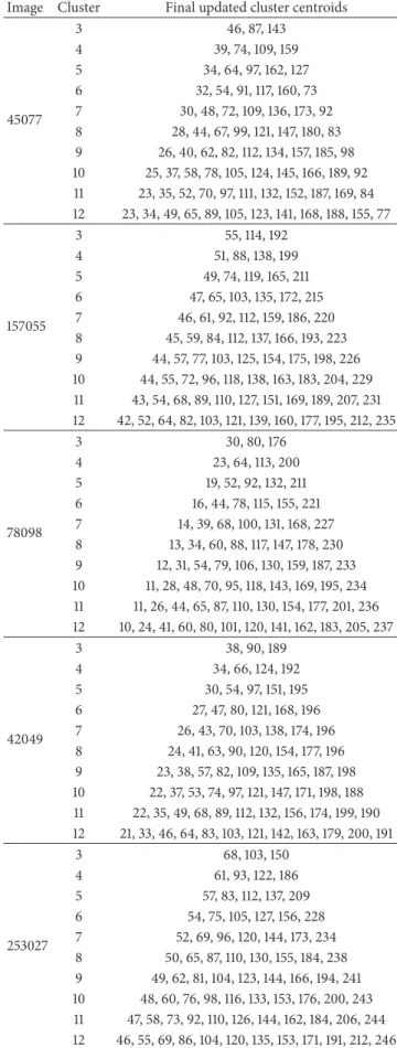
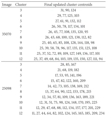
Table 2 shows the final updated cluster centroids for
clusters 3 to 12 for all the test images used in this study. These
values were computed based on (9). The cluster centroid
update procedure based on these equations can be deemed successful as reflected in the visual result of the segmentation.
For instance, in Table 2, the initial centroids of the image
“45077” for four clusters, which were 9, 69, 129, and 189, were updated to the final values of 39, 74, 109, and 159, showing that an update was actually performed. Similar results were obtained for all the other test images used in this study
as shown in Table 2. The updated cluster centroids finally
computed by the proposed algorithm tend towards the higher pixel intensity value in the input as the number of clusters is increased. This significantly contributes to the enhancement of the segmentation result in higher clusters. These values of
Table 2: Final updated cluster centroids. Image Cluster Final updated cluster centroids
45077 3 46, 87, 143 4 39, 74, 109, 159 5 34, 64, 97, 162, 127 6 32, 54, 91, 117, 160, 73 7 30, 48, 72, 109, 136, 173, 92 8 28, 44, 67, 99, 121, 147, 180, 83 9 26, 40, 62, 82, 112, 134, 157, 185, 98 10 25, 37, 58, 78, 105, 124, 145, 166, 189, 92 11 23, 35, 52, 70, 97, 111, 132, 152, 187, 169, 84 12 23, 34, 49, 65, 89, 105, 123, 141, 168, 188, 155, 77 157055 3 55, 114, 192 4 51, 88, 138, 199 5 49, 74, 119, 165, 211 6 47, 65, 103, 135, 172, 215 7 46, 61, 92, 112, 159, 186, 220 8 45, 59, 84, 112, 137, 166, 193, 223 9 44, 57, 77, 103, 125, 154, 175, 198, 226 10 44, 55, 72, 96, 118, 138, 163, 183, 204, 229 11 43, 54, 68, 89, 110, 127, 151, 169, 189, 207, 231 12 42, 52, 64, 82, 103, 121, 139, 160, 177, 195, 212, 235 78098 3 30, 80, 176 4 23, 64, 113, 200 5 19, 52, 92, 132, 211 6 16, 44, 78, 115, 155, 221 7 14, 39, 68, 100, 131, 168, 227 8 13, 34, 60, 88, 117, 147, 178, 230 9 12, 31, 54, 79, 106, 130, 159, 187, 233 10 11, 28, 48, 70, 95, 118, 143, 169, 195, 234 11 11, 26, 44, 65, 87, 110, 130, 154, 177, 201, 236 12 10, 24, 41, 60, 80, 101, 120, 141, 162, 183, 205, 237 42049 3 38, 90, 189 4 34, 66, 124, 192 5 30, 54, 97, 151, 195 6 27, 47, 80, 121, 168, 196 7 26, 43, 70, 103, 138, 174, 196 8 24, 41, 63, 90, 120, 154, 177, 196 9 23, 38, 57, 82, 109, 135, 165, 187, 198 10 22, 37, 53, 74, 97, 121, 147, 171, 198, 188 11 22, 35, 49, 68, 89, 112, 132, 156, 174, 199, 190 12 21, 33, 46, 64, 83, 103, 121, 142, 163, 179, 200, 191 253027 3 68, 103, 150 4 61, 93, 122, 186 5 57, 83, 112, 137, 209 6 54, 75, 105, 127, 156, 228 7 52, 69, 96, 120, 144, 173, 234 8 50, 65, 87, 110, 130, 155, 184, 238 9 49, 62, 81, 104, 123, 144, 166, 194, 241 10 48, 60, 76, 98, 116, 133, 153, 176, 200, 243 11 47, 58, 73, 92, 110, 126, 144, 162, 184, 206, 244 12 46, 55, 69, 86, 104, 120, 135, 153, 171, 191, 212, 246
Table 2: Continued.
Image Cluster Final updated cluster centroids
169012 3 48, 92, 183 4 44, 73, 125, 201 5 41, 64, 104, 148, 211 6 39, 58, 90, 127, 166, 218 7 37, 54, 79, 112, 145, 178, 222 8 35, 51, 72, 100, 129, 159, 188, 227 9 34, 49, 67, 91, 117, 142, 169, 195, 230 10 33, 46, 62, 84, 107, 131, 154, 178, 202, 233 11 32, 44, 59, 77, 99, 120, 141, 163, 185, 206, 235 12 31, 43, 56, 73, 92, 112, 132, 151, 171, 191, 210, 237 210088 3 68, 99, 175 4 62, 89, 125, 186 5 56, 80, 105, 149, 196 6 53, 74, 97, 130, 168, 207 7 50, 70, 92, 115, 149, 178, 213 8 48, 66, 85, 104, 133, 162, 187, 220 9 47, 63, 81, 98, 120, 147, 173, 195, 224 10 46, 60, 77, 94, 112, 135, 159, 180, 200, 227 11 45, 58, 73, 89, 104, 123, 146, 167, 186, 205, 230 12 45, 55, 70, 85, 100, 117, 136, 156, 174, 191, 208, 232 208001 3 40, 81, 157 4 35, 69, 109, 181 5 32, 59, 91, 130, 195 6 30, 51, 80, 113, 152, 211 7 28, 45, 72, 99, 130, 164, 218 8 26, 39, 64, 88, 116, 147, 176, 224 9 24, 35, 58, 80, 104, 130, 158, 185, 229 10 21, 33, 52, 74, 95, 119, 143, 167, 191, 231 11 20, 31, 48, 68, 88, 109, 130, 154, 176, 197, 233 12 19, 31, 46, 64, 81, 100, 120, 141, 162, 182, 203, 235 10081 3 48, 104, 164 4 38, 74, 122, 166 5 32, 60, 107, 152, 181 6 27, 54, 89, 127, 177, 153 7 25, 48, 75, 110, 148, 185, 163 8 23, 43, 66, 95, 127, 153, 187, 167 9 21, 40, 61, 87, 115, 146, 171, 193, 159 10 20, 36, 55, 78, 100, 125, 150, 177, 205, 164 11 19, 34, 50, 69, 93, 117, 142, 164, 178, 208, 154 12 18, 31, 48, 65, 86, 105, 126, 148, 169, 181, 211, 159 155060 3 43, 83, 187 4 35, 68, 111, 212 5 29, 56, 91, 131, 220 6 23, 49, 80, 113, 150, 223 7 19, 44, 70, 99, 129, 168, 226 8 17, 39, 62, 89, 117, 145, 185, 228 9 15, 36, 56, 80, 105, 129, 156, 194, 229 10 14, 33, 51, 72, 95, 119, 142, 169, 201, 231 11 13, 31, 48, 67, 88, 109, 129, 151, 179, 208, 232 12 12, 29, 44, 61, 80, 100, 119, 139, 161, 186, 211, 233 Table 2: Continued.
Image Cluster Final updated cluster centroids
35070 3 31, 90, 124 4 29, 77, 125, 103 5 27, 61, 91, 132, 112 6 26, 50, 78, 117, 134, 101 7 26, 45, 77, 108, 135, 120, 95 8 26, 43, 68, 100, 121, 138, 112, 82 9 25, 40, 65, 85, 108, 128, 144, 118, 98 10 25, 39, 58, 78, 96, 117, 135, 151, 125, 108 11 25, 37, 52, 72, 89, 109, 127, 149, 136, 117, 101 12 25, 37, 49, 68, 84, 103, 119, 135, 150, 127, 111, 94 25098 3 28, 85, 167 4 21, 68, 119, 182 5 17, 53, 93, 141, 196 6 15, 47, 82, 122, 160, 209 7 14, 42, 73, 105, 138, 169, 212 8 13, 37, 64, 90, 122, 153, 178, 215 9 12, 34, 57, 81, 109, 136, 163, 189, 221 10 12, 31, 51, 75, 98, 124, 148, 170, 195, 225 11 12, 29, 47, 68, 88, 112, 134, 157, 177, 201, 229 12 11, 27, 44, 64, 82, 102, 124, 145, 165, 185, 209, 234
the updated cluster centroids are ultimately used to compute the output images in the final step of PICA.
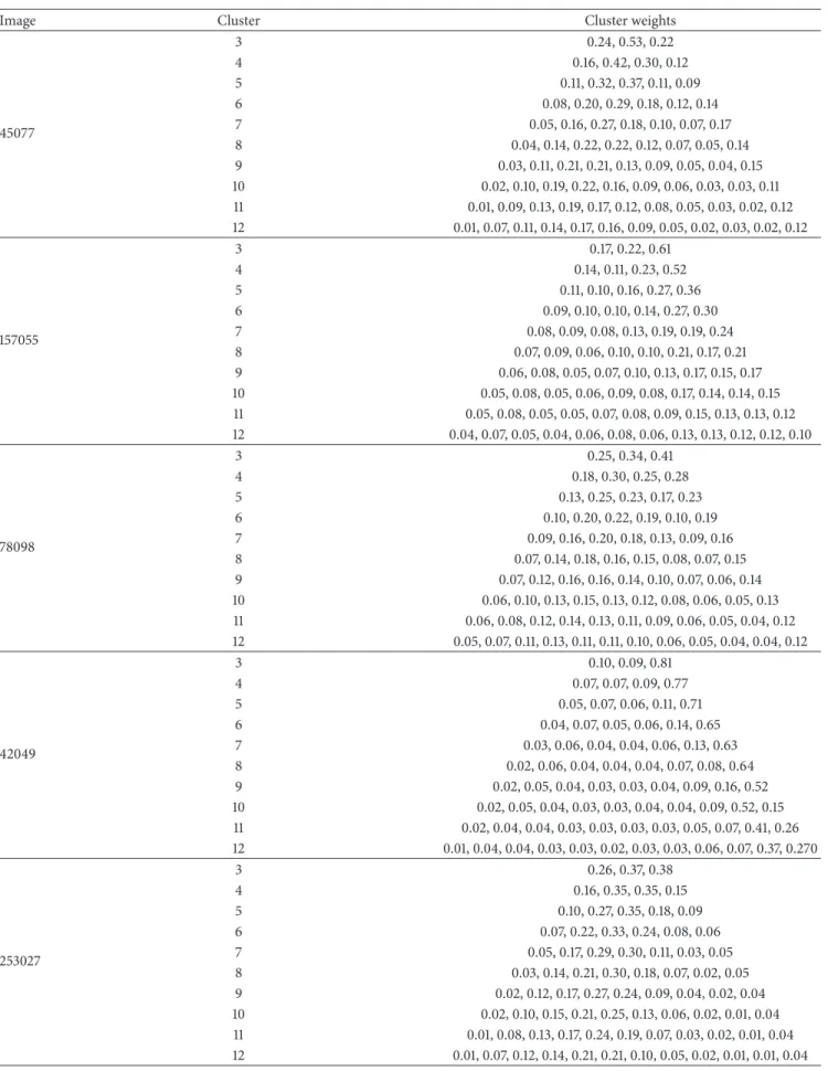
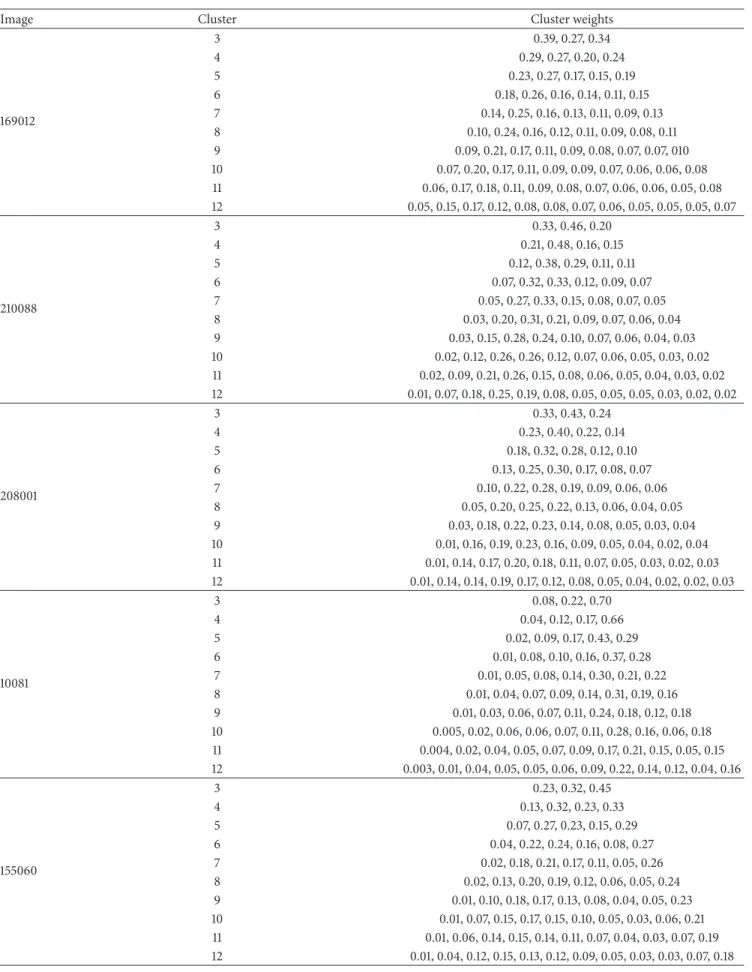
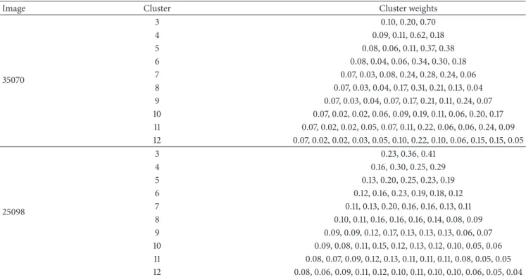
Table 3shows the weights of clusters from 3 to 12 for all
the test images in this study. It can be noted inTable 3for
all the images that cluster weights for a particular image add up to unity. This is in perfect agreement with the probability
theory in(10). In codicil, it can be observed inTable 3that
no cluster weight for all the test images is equal to zero. This implies that there is no possibility for the algorithm to break down at any number of clusters and there is no incidence of empty clusters, which can result in the dead centers syndrome using the proposed algorithm.
4.3. Comparative Results. In this section, we adopted both qualitative (subjective) and quantitative (objective) evalua-tions to compare the segmentation results of the proposed algorithm with KM, PSO, DPSO, and FODPSO segmentation algorithms. These existing algorithms were selected because KM clustering is reported to be one of the most prevalent clustering algorithms due to its implementation simplicity and low computational costs. The PSO-based segmentation methods (PSO, DPSO, and FODPSO) were also shown in the literature to act better than other metaheuristic methods in
terms of precision, robustness of results, and runtime [28,37].
4.3.1. Qualitative. Qualitative evaluation on the basis of human visual perception is a widely used strategy in the literature to carry out performance assessment of image segmentation algorithms [29]. The original grayscale images selected from the Berkeley Segmentation Dataset and
Bench-mark for evaluations are labelled as (a) in Figures1–12while
Table 3: Cluster weights.
Image Cluster Cluster weights
45077 3 0.24, 0.53, 0.22 4 0.16, 0.42, 0.30, 0.12 5 0.11, 0.32, 0.37, 0.11, 0.09 6 0.08, 0.20, 0.29, 0.18, 0.12, 0.14 7 0.05, 0.16, 0.27, 0.18, 0.10, 0.07, 0.17 8 0.04, 0.14, 0.22, 0.22, 0.12, 0.07, 0.05, 0.14 9 0.03, 0.11, 0.21, 0.21, 0.13, 0.09, 0.05, 0.04, 0.15 10 0.02, 0.10, 0.19, 0.22, 0.16, 0.09, 0.06, 0.03, 0.03, 0.11 11 0.01, 0.09, 0.13, 0.19, 0.17, 0.12, 0.08, 0.05, 0.03, 0.02, 0.12 12 0.01, 0.07, 0.11, 0.14, 0.17, 0.16, 0.09, 0.05, 0.02, 0.03, 0.02, 0.12 157055 3 0.17, 0.22, 0.61 4 0.14, 0.11, 0.23, 0.52 5 0.11, 0.10, 0.16, 0.27, 0.36 6 0.09, 0.10, 0.10, 0.14, 0.27, 0.30 7 0.08, 0.09, 0.08, 0.13, 0.19, 0.19, 0.24 8 0.07, 0.09, 0.06, 0.10, 0.10, 0.21, 0.17, 0.21 9 0.06, 0.08, 0.05, 0.07, 0.10, 0.13, 0.17, 0.15, 0.17 10 0.05, 0.08, 0.05, 0.06, 0.09, 0.08, 0.17, 0.14, 0.14, 0.15 11 0.05, 0.08, 0.05, 0.05, 0.07, 0.08, 0.09, 0.15, 0.13, 0.13, 0.12 12 0.04, 0.07, 0.05, 0.04, 0.06, 0.08, 0.06, 0.13, 0.13, 0.12, 0.12, 0.10 78098 3 0.25, 0.34, 0.41 4 0.18, 0.30, 0.25, 0.28 5 0.13, 0.25, 0.23, 0.17, 0.23 6 0.10, 0.20, 0.22, 0.19, 0.10, 0.19 7 0.09, 0.16, 0.20, 0.18, 0.13, 0.09, 0.16 8 0.07, 0.14, 0.18, 0.16, 0.15, 0.08, 0.07, 0.15 9 0.07, 0.12, 0.16, 0.16, 0.14, 0.10, 0.07, 0.06, 0.14 10 0.06, 0.10, 0.13, 0.15, 0.13, 0.12, 0.08, 0.06, 0.05, 0.13 11 0.06, 0.08, 0.12, 0.14, 0.13, 0.11, 0.09, 0.06, 0.05, 0.04, 0.12 12 0.05, 0.07, 0.11, 0.13, 0.11, 0.11, 0.10, 0.06, 0.05, 0.04, 0.04, 0.12 42049 3 0.10, 0.09, 0.81 4 0.07, 0.07, 0.09, 0.77 5 0.05, 0.07, 0.06, 0.11, 0.71 6 0.04, 0.07, 0.05, 0.06, 0.14, 0.65 7 0.03, 0.06, 0.04, 0.04, 0.06, 0.13, 0.63 8 0.02, 0.06, 0.04, 0.04, 0.04, 0.07, 0.08, 0.64 9 0.02, 0.05, 0.04, 0.03, 0.03, 0.04, 0.09, 0.16, 0.52 10 0.02, 0.05, 0.04, 0.03, 0.03, 0.04, 0.04, 0.09, 0.52, 0.15 11 0.02, 0.04, 0.04, 0.03, 0.03, 0.03, 0.03, 0.05, 0.07, 0.41, 0.26 12 0.01, 0.04, 0.04, 0.03, 0.03, 0.02, 0.03, 0.03, 0.06, 0.07, 0.37, 0.270 253027 3 0.26, 0.37, 0.38 4 0.16, 0.35, 0.35, 0.15 5 0.10, 0.27, 0.35, 0.18, 0.09 6 0.07, 0.22, 0.33, 0.24, 0.08, 0.06 7 0.05, 0.17, 0.29, 0.30, 0.11, 0.03, 0.05 8 0.03, 0.14, 0.21, 0.30, 0.18, 0.07, 0.02, 0.05 9 0.02, 0.12, 0.17, 0.27, 0.24, 0.09, 0.04, 0.02, 0.04 10 0.02, 0.10, 0.15, 0.21, 0.25, 0.13, 0.06, 0.02, 0.01, 0.04 11 0.01, 0.08, 0.13, 0.17, 0.24, 0.19, 0.07, 0.03, 0.02, 0.01, 0.04 12 0.01, 0.07, 0.12, 0.14, 0.21, 0.21, 0.10, 0.05, 0.02, 0.01, 0.01, 0.04
Table 3: Continued.
Image Cluster Cluster weights
169012 3 0.39, 0.27, 0.34 4 0.29, 0.27, 0.20, 0.24 5 0.23, 0.27, 0.17, 0.15, 0.19 6 0.18, 0.26, 0.16, 0.14, 0.11, 0.15 7 0.14, 0.25, 0.16, 0.13, 0.11, 0.09, 0.13 8 0.10, 0.24, 0.16, 0.12, 0.11, 0.09, 0.08, 0.11 9 0.09, 0.21, 0.17, 0.11, 0.09, 0.08, 0.07, 0.07, 010 10 0.07, 0.20, 0.17, 0.11, 0.09, 0.09, 0.07, 0.06, 0.06, 0.08 11 0.06, 0.17, 0.18, 0.11, 0.09, 0.08, 0.07, 0.06, 0.06, 0.05, 0.08 12 0.05, 0.15, 0.17, 0.12, 0.08, 0.08, 0.07, 0.06, 0.05, 0.05, 0.05, 0.07 210088 3 0.33, 0.46, 0.20 4 0.21, 0.48, 0.16, 0.15 5 0.12, 0.38, 0.29, 0.11, 0.11 6 0.07, 0.32, 0.33, 0.12, 0.09, 0.07 7 0.05, 0.27, 0.33, 0.15, 0.08, 0.07, 0.05 8 0.03, 0.20, 0.31, 0.21, 0.09, 0.07, 0.06, 0.04 9 0.03, 0.15, 0.28, 0.24, 0.10, 0.07, 0.06, 0.04, 0.03 10 0.02, 0.12, 0.26, 0.26, 0.12, 0.07, 0.06, 0.05, 0.03, 0.02 11 0.02, 0.09, 0.21, 0.26, 0.15, 0.08, 0.06, 0.05, 0.04, 0.03, 0.02 12 0.01, 0.07, 0.18, 0.25, 0.19, 0.08, 0.05, 0.05, 0.05, 0.03, 0.02, 0.02 208001 3 0.33, 0.43, 0.24 4 0.23, 0.40, 0.22, 0.14 5 0.18, 0.32, 0.28, 0.12, 0.10 6 0.13, 0.25, 0.30, 0.17, 0.08, 0.07 7 0.10, 0.22, 0.28, 0.19, 0.09, 0.06, 0.06 8 0.05, 0.20, 0.25, 0.22, 0.13, 0.06, 0.04, 0.05 9 0.03, 0.18, 0.22, 0.23, 0.14, 0.08, 0.05, 0.03, 0.04 10 0.01, 0.16, 0.19, 0.23, 0.16, 0.09, 0.05, 0.04, 0.02, 0.04 11 0.01, 0.14, 0.17, 0.20, 0.18, 0.11, 0.07, 0.05, 0.03, 0.02, 0.03 12 0.01, 0.14, 0.14, 0.19, 0.17, 0.12, 0.08, 0.05, 0.04, 0.02, 0.02, 0.03 10081 3 0.08, 0.22, 0.70 4 0.04, 0.12, 0.17, 0.66 5 0.02, 0.09, 0.17, 0.43, 0.29 6 0.01, 0.08, 0.10, 0.16, 0.37, 0.28 7 0.01, 0.05, 0.08, 0.14, 0.30, 0.21, 0.22 8 0.01, 0.04, 0.07, 0.09, 0.14, 0.31, 0.19, 0.16 9 0.01, 0.03, 0.06, 0.07, 0.11, 0.24, 0.18, 0.12, 0.18 10 0.005, 0.02, 0.06, 0.06, 0.07, 0.11, 0.28, 0.16, 0.06, 0.18 11 0.004, 0.02, 0.04, 0.05, 0.07, 0.09, 0.17, 0.21, 0.15, 0.05, 0.15 12 0.003, 0.01, 0.04, 0.05, 0.05, 0.06, 0.09, 0.22, 0.14, 0.12, 0.04, 0.16 155060 3 0.23, 0.32, 0.45 4 0.13, 0.32, 0.23, 0.33 5 0.07, 0.27, 0.23, 0.15, 0.29 6 0.04, 0.22, 0.24, 0.16, 0.08, 0.27 7 0.02, 0.18, 0.21, 0.17, 0.11, 0.05, 0.26 8 0.02, 0.13, 0.20, 0.19, 0.12, 0.06, 0.05, 0.24 9 0.01, 0.10, 0.18, 0.17, 0.13, 0.08, 0.04, 0.05, 0.23 10 0.01, 0.07, 0.15, 0.17, 0.15, 0.10, 0.05, 0.03, 0.06, 0.21 11 0.01, 0.06, 0.14, 0.15, 0.14, 0.11, 0.07, 0.04, 0.03, 0.07, 0.19 12 0.01, 0.04, 0.12, 0.15, 0.13, 0.12, 0.09, 0.05, 0.03, 0.03, 0.07, 0.18
Table 3: Continued.
Image Cluster Cluster weights
35070 3 0.10, 0.20, 0.70 4 0.09, 0.11, 0.62, 0.18 5 0.08, 0.06, 0.11, 0.37, 0.38 6 0.08, 0.04, 0.06, 0.34, 0.30, 0.18 7 0.07, 0.03, 0.08, 0.24, 0.28, 0.24, 0.06 8 0.07, 0.03, 0.04, 0.17, 0.31, 0.21, 0.13, 0.04 9 0.07, 0.03, 0.04, 0.07, 0.17, 0.21, 0.11, 0.24, 0.07 10 0.07, 0.02, 0.02, 0.06, 0.09, 0.19, 0.11, 0.06, 0.20, 0.17 11 0.07, 0.02, 0.02, 0.05, 0.07, 0.11, 0.22, 0.06, 0.06, 0.24, 0.09 12 0.07, 0.02, 0.02, 0.03, 0.05, 0.10, 0.22, 0.10, 0.06, 0.15, 0.15, 0.05 25098 3 0.23, 0.36, 0.41 4 0.16, 0.30, 0.25, 0.29 5 0.13, 0.20, 0.25, 0.23, 0.19 6 0.12, 0.16, 0.23, 0.19, 0.18, 0.12 7 0.11, 0.13, 0.20, 0.16, 0.16, 0.13, 0.11 8 0.10, 0.11, 0.16, 0.16, 0.16, 0.14, 0.08, 0.09 9 0.09, 0.09, 0.12, 0.17, 0.13, 0.13, 0.13, 0.06, 0.07 10 0.09, 0.08, 0.11, 0.15, 0.12, 0.13, 0.12, 0.10, 0.05, 0.06 11 0.08, 0.07, 0.09, 0.12, 0.13, 0.11, 0.11, 0.11, 0.08, 0.05, 0.05 12 0.08, 0.06, 0.09, 0.11, 0.12, 0.10, 0.11, 0.10, 0.10, 0.06, 0.05, 0.04 (a) (b) (c) (d) (e) (f)
Figure 1: Segmentation results in 3 clusters/levels of image “45077” after applying different algorithms: (a) original image, (b) KM, (c) PSO, (d) DPSO, (e) FODPSO, and (f) proposed.
DPSO, FODPSO, and the proposed algorithm are labelled as (b) to (f), respectively. The number of clusters for segmenting each of the test images varied from 3 to 14. Worthy of note is the fact that, based on visual appeal, the segmentation outputs of all the conventional algorithms and our proposed algorithm are only fairly acceptable at cluster/level 3. In
general, there were improvements in the visual appeal of the outputs of the conventional algorithms and the proposed algorithm as we increased the number of clusters/levels from 4 up to 14. However, it can be observed that there are several white patches in the outputs of the KM algorithm
(a) (b) (c)
(d) (e) (f)
Figure 2: Segmentation results in 4 clusters/levels of image “157055” after applying different algorithms: (a) original image, (b) KM, (c) PSO, (d) DPSO, (e) FODPSO, and (f) proposed.
(a) (b) (c)
(d) (e) (f)
Figure 3: Segmentation results in 5 clusters/levels of image “78098” after applying different algorithms: (a) original image, (b) KM, (c) PSO, (d) DPSO, (e) FODPSO, and (f) proposed.
11. The segmentation outputs of PSO, DPSO, and FODPSO algorithms also have a lot of black patches as noticeably
shown in Figures 2, 3, 4, 5, 6, 7, 8, 11, and 12. Conversely,
the output of the proposed algorithm is shown across the entire test images and from clusters 4 to 14 to be more visually appealing because no white or black patches are found in any of the results. This qualitative evaluation clearly shows that our algorithm achieved more homogeneous segmenta-tion outputs than the other comparative algorithms in this study. Quantitative evaluation is further carried out for the
selected test images using the conventional algorithms and the proposed algorithm.
4.3.2. Quantitative. Quantitative evaluation objectively com-putes the performance of segmentation algorithms with appropriate similarity metrics and it is not subject to human errors like in the qualitative evaluation method. Conse-quently, for the quantitative aspect of this study, we employed some metrics to compare the proposed algorithm with the
(a) (b) (c)
(d) (e) (f)
Figure 4: Segmentation results in 6 clusters/levels of image “42049” after applying different algorithms: (a) original image, (b) KM, (c) PSO, (d) DPSO, (e) FODPSO, and (f) proposed.
(a) (b) (c)
(d) (e) (f)
Figure 5: Segmentation results in 7 clusters/levels of image “253027” after applying different algorithms: (a) original image, (b) KM, (c) PSO, (d) DPSO, (e) FODPSO, and (f) proposed.
and the Structural Similarity Measure (SSIM). The maximum Jaccard index and SSIM of 1 are only achieved if the two images are identical. These similarity metrics (Jaccard and SSIM) can be mathematically defined in terms of two images
𝑥 = {𝑥𝑖| 𝑖 = 1, . . . 𝑀}and y= {𝑦𝑖| 𝑖 = 1, . . . 𝑁}.
Given that|𝑥|denotes the cardinality of image𝑥, which
is a count of the number of elements that are present in x, the
Jaccard similarity index between the two images𝑥and𝑦is
given as [49]
𝐽 (𝑥, 𝑦) = 𝑥 ∩ 𝑦𝑥 ∪ 𝑦, (11)
where𝑥 ∩ 𝑦denotes the intersection between the two images
(a) (b) (c)
(d) (e) (f)
Figure 6: Segmentation results in 8 clusters/levels of image “169012” after applying different algorithms: (a) original image, (b) KM, (c) PSO, (d) DPSO, (e) FODPSO, and (f) proposed.
(a) (b) (c)
(d) (e) (f)
Figure 7: Segmentation results in 9 clusters/levels of image “210088” after applying different algorithms: (a) original image, (b) KM, (c) PSO, (d) DPSO, (e) FODPSO, and (f) proposed.
denotes the union between the two images and represents all elements that are in either of them.
The SSIM index was proposed to predict human pref-erences in image quality assessment. To compute SSIM,
the means (𝜇𝑥, 𝜇𝑦), the variances (𝜎𝑥2, 𝜎𝑦2), and the
cross-covariance (𝜎𝑥𝑦) of images x and y are first computed and are
based on these values, and the SSIM between images x and y is given as [50]
𝑆 (𝑥, 𝑦) = (2𝜇𝑥𝜇𝑦+ 𝐶1) (2𝜎𝑥𝑦+ 𝐶2) (𝜇2
𝑥+ 𝜇𝑦2+ 𝐶1) (𝜎𝑥2+ 𝜎2𝑦+ 𝐶2)
(a) (b) (c)
(d) (e) (f)
Figure 8: Segmentation results in 10 clusters/levels of image “208001” after applying different algorithms: (a) original image, (b) KM, (c) PSO, (d) DPSO, (e) FODPSO, and (f) proposed.
(a) (b) (c)
(d) (e) (f)
Figure 9: Segmentation results in 11 clusters/levels of image “10081” after applying different algorithms: (a) original image, (b) KM, (c) PSO, (d) DPSO, (e) FODPSO, and (f) proposed.
where𝐶1and𝐶2are small positive constants,𝜇𝑥is the mean
of𝑥, and𝜎𝑥2is the variance.
The values obtained for these metrics in (11) and (12)
when applied to the test images for clusters 3 to 14 are shown
in Table 4. As shown in the table, both the Jaccard index
and the SSIM index for the proposed algorithm improved progressively from cluster 3 up to cluster 14 for the different test images. In addition, the results of the two metrics for the proposed algorithm are better than the values obtained for the other algorithms compared from clusters/levels 3 up to
14 across all the test images (Table 4). These results further consolidate the qualitative comparison result, which earlier established that our proposed algorithm performs better than KM, PSO, DPSO, and FODPSO. The computed evaluation metrics also indicate that the values of the SSIM indices are consistently higher than the values of Jaccard indices for all the test images from clusters/levels 3 up to 14. For instance,
at cluster 3 in Table 4, the Jaccard index for the proposed
algorithm is 0.8639 while that of the SSIM index is 0.8979 and at cluster 14, the value of the Jaccard index is 0.9603
(a) (b) (c)
(d) (e) (f)
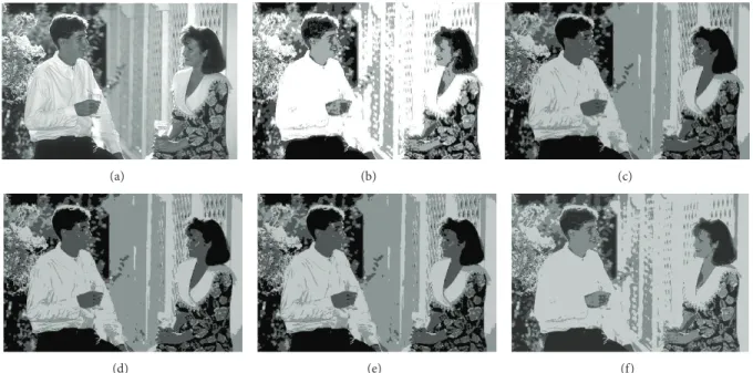
Figure 10: Segmentation results in 12 clusters/levels of image “155060” after applying different algorithms: (a) original image, (b) KM, (c) PSO, (d) DPSO, (e) FODPSO, and (f) proposed.
(a) (b) (c)
(d) (e) (f)
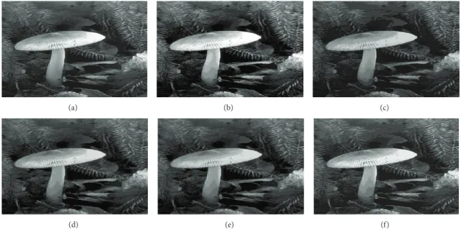
Figure 11: Segmentation results in 13 clusters/levels of image “35070” after applying different algorithms: (a) original image, (b) KM, (c) PSO, (d) DPSO, (e) FODPSO, and (f) proposed.
while that of the SSIM index is 0.9965. A similar trend was observed for all the conventional algorithms, even though the values obtained from the two metrics were lower for the conventional algorithms than the proposed algorithm. Apparently, the SSIM index value of 0.9965 obtained for the proposed algorithm at cluster 14 is a better quantitative representation of the visual appeal of the segmented image than the Jaccard index value of 0.9603. We can therefore safely infer that, based on the evaluations carried out in this study, the SSIM index is a better measure of similarity between an
input image and a segmented image than the Jaccard index. Hence, the SSIM evaluation metric is highly promising for many other post-image segmentation processing tasks such as object features extraction and content retrieval.
5. Conclusion
In this study, a new clustering algorithm was proposed and applied to multilevel image segmentation problem. The objectives of the proposed algorithm were to improve the
(a) (b) (c)
(d) (e) (f)
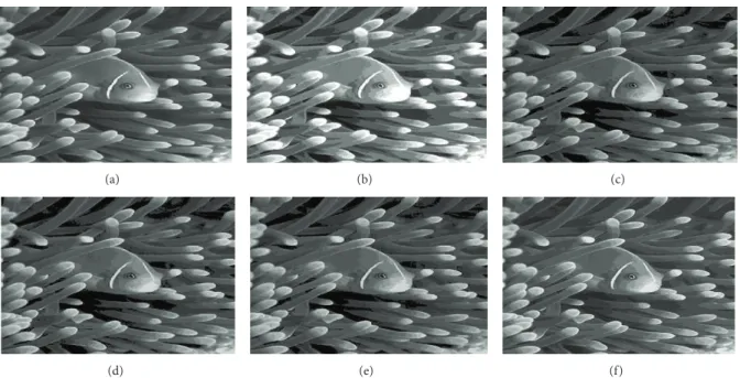
Figure 12: Segmentation results in 14 clusters/levels of image “25098” after applying different algorithms: (a) original image, (b) KM, (c) PSO, (d) DPSO, (e) FODPSO, and (f) proposed.
Table 4: Comparative results.
Image 𝑄 Clusters Metrics KM PSO DPSO FODPSO Proposed
45077 240 3 Jaccard 0.5560 0.6257 0.5963 0.6251 0.8639 SSIM 0.7682 0.6917 0.6756 0.7220 0.8979 157055 223 4 Jaccard 0.8081 0.7881 0.7889 0.7889 0.9004 SSIM 0.8204 0.8091 0.8082 0.8082 0.9418 78098 253 5 Jaccard 0.8303 0.7682 0.7682 0.7685 0.8802 SSIM 0.8569 0.7324 0.7324 0.8229 0.9669 42049 233 6 Jaccard 0.8465 0.9212 0.9213 0.9213 0.9646 SSIM 0.9082 0.9238 0.9237 0.9237 0.9894 253027 222 7 Jaccard 0.7956 0.8427 0.8347 0.8573 0.9410 SSIM 0.8791 0.9113 0.8997 0.9356 0.9787 169012 235 8 Jaccard 0.8272 0.8391 0.8307 0.8306 0.9377 SSIM 0.7983 0.8530 0.8312 0.8311 0.9910 210088 221 9 Jaccard 0.8214 0.8876 0.8778 0.8960 0.9521 SSIM 0.9655 0.9329 0.9183 0.9643 0.9894 208001 247 10 Jaccard 0.8210 0.8581 0.8624 0.8581 0.9383 SSIM 0.8272 0.8814 0.8940 0.8806 0.9911 10081 249 11 Jaccard 0.9157 0.9350 0.9395 0.9401 0.9681 SSIM 0.9765 0.9872 0.9761 0.9766 0.9881 155060 253 12 Jaccard 0.9080 0.9257 0.9246 0.9229 0.9592 SSIM 0.9465 0.9797 0.9751 0.9760 0.9965 35070 204 13 Jaccard 0.7240 0.8411 0.9133 0.9093 0.9770 SSIM 0.8501 0.9606 0.9176 0.9167 0.9937 25098 252 14 Jaccard 0.8218 0.8071 0.8320 0.8324 0.9603 SSIM 0.8845 0.9335 0.9188 0.9523 0.9965
initialization of cluster centroids and the allocation of pixel intensities into clusters. This is to eliminate the dead center problem and inappropriate pixel allocation to clusters as commonly encountered in many of the existing clustering based multilevel segmentation methods. The simple math-ematical concepts utilized in achieving the objectives are linear partitioning of the pixel intensity set and between-cluster variance criterion function. The new multilevel seg-mentation algorithm is conceptually simple, robust, and computationally cost effective. The algorithm was compared with KM, PSO, DPSO, and FODPSO on 12 real images from the Berkeley Segmentation Dataset and Benchmark. The qualitative results show that the proposed algorithm consistently produced patch-free segmentation, unlike the other existing algorithms. The quantitative results using the Jaccard index and the SSIM show that the segmentation results of our algorithm improve with increasing number of clusters across different images without a corresponding increase in computational cost, unlike the other algorithms. Our experiments further showed that when the number of
clusters 𝐾 is equal to the number of pixel intensities 𝑄,
(𝐾 = 𝑄 and 𝑄 ≤ 256), the value of SSIM becomes 1, which is a confirmation of the survivability and recoverability capabilities of the algorithm. On the contrary, the other comparative algorithms in this study either break down or
become unbearably slow for𝐾 > 180. This study opens new
perspective on multilevel image segmentation because mul-tilevel thresholding algorithms were previously considered suitable for solving multilevel image segmentation problem. Future work will involve a search for better initialization schemes and pixel intensities allocation concepts to further enhance the performance of the algorithm.
Conflict of Interests
The authors declare that there is no conflict of interests regarding the publication of this paper.
Acknowledgment
E. Adetiba is on postdoctoral fellowship at the ICT and Society (ICTAS) Research Group, Durban University of Technology, South Africa, funded by the Durban University of Technology Research and Development Directorate. He is on postdoctoral research leave from the Department of Elec-trical & Information Engineering, College of Engineering, Covenant University, Ota, Ogun State, Nigeria.
References
[1] A. Alihodzic and M. Tuba, “Improved bat algorithm applied to multilevel image thresholding,”The Scientific World Journal, vol. 2014, Article ID 176718, 16 pages, 2014.
[2] M. H. J. Vala and A. Baxi, “A review on Otsu image segmenta-tion algorithm,”International Journal of Advanced Research in Computer Engineering & Technology, vol. 2, no. 2, pp. 387–389, 2013.
[3] C. A. Glasbey and G. W. Horgan, Image Analysis for the Biological Sciences, vol. 1, Wiley, Chichester, UK, 1995.
[4] D. A. Okuboyejo, O. O. Olugbara, and S. A. Odunaike, “CLAHE inspired segmentation of dermoscopic images using mixture of methods,” inTransactions on Engineering Technologies, pp. 355– 365, Springer, Dordrecht, The Netherlands, 2014.
[5] S. A. Daramola, E. Adetiba, A. U. Adoghe, J. A. Badejo, I. A. Samuel, and T. Fagorusi, “Automatic vehicle identification system using license plate,”International Journal of Engineering Science and Technology, vol. 3, no. 2, pp. 1712–1719, 2011. [6] Y. Ramadevi, T. Sridevi, B. Poornima, and B. Kalyani,
“Segmen-tation and object recognition using edge detection technique,” International Journal of Computer Science & Information Tech-nology, vol. 2, no. 6, pp. 153–161, 2010.
[7] D. Oliva, E. Cuevas, G. Pajares, D. Zaldivar, and V. Osuna, “A multilevel thresholding algorithm using electro-magnetism optimization,”Neurocomputing, vol. 139, pp. 357–381, 2014. [8] B. T. Abe, O. O. Olugbara, and T. Marwala, “Experimental
comparison of support vector machines with random forests for hyperspectral image land cover classification,”Journal of Earth System Science, vol. 123, no. 4, pp. 779–790, 2014.
[9] H. B. Kekre and S. M. Gharge, “Image segmentation using extended edge operator for mammographic images,” Interna-tional Journal on Computer Science and Engineering, vol. 2, no. 4, pp. 1086–1091, 2010.
[10] G. C. Lekhana and R. Srikantaswamy, “Real time license plate recognition system,” International Journal of Advanced Technology & Engineering Research, vol. 2, no. 4, pp. 5–9, 2012. [11] T. Zuva, O. O. Olugbara, S. O. Ojo, and S. M. Ngwira, “Image
segmentation, available techniques, developments and open issues,”Canadian Journal on Image Processing and Computer Vision, vol. 2, no. 3, pp. 20–29, 2011.
[12] M. Juneja and P. S. Sandhu, “Performance evaluation of edge detection techniques for images in spatial domain,” Interna-tional Journal of Computer Theory and Engineering, vol. 1, no. 5, pp. 614–621, 2009.
[13] M. A. El-Sayed, “A new algorithm based entropic threshold for edge detection in images,”International Journal of Computer Science Issues, vol. 8, no. 1, pp. 71–78, 2011.
[14] H. D. Cheng, X. H. Jiang, Y. Sun, and J. Wang, “Color image segmentation: advances and prospects,” Pattern Recognition, vol. 34, no. 12, pp. 2259–2281, 2001.
[15] Y.-H. Kuan, C.-M. Kuo, and N.-C. Yang, “Color-based image salient region segmentation using novel region merging strat-egy,”IEEE Transactions on Multimedia, vol. 10, no. 5, pp. 832– 845, 2008.
[16] R. C. Gonzalez and R. E. Woods, Digital Image Processing, Publishing House of Electronics Industry, Beijing, China, 2nd edition, 2007.
[17] V. Osuna-Enciso, E. Cuevas, and H. Sossa, “A comparison of nature inspired algorithms for multi-threshold image segmen-tation,”Expert Systems with Applications, vol. 40, no. 4, pp. 1213– 1219, 2013.
[18] L. Dong, G. Yu, P. Ogunbona, and W. Li, “An efficient iterative algorithm for image thresholding,”Pattern Recognition Letters, vol. 29, no. 9, pp. 1311–1316, 2008.
[19] P.-S. Liao, T.-S. Chen, and P.-C. Chung, “A fast algorithm for multilevel thresholding,” Journal of Information Science and Engineering, vol. 17, no. 5, pp. 713–727, 2001.
[20] X. Yang, X. Shen, J. Long, and H. Chen, “An improved median-based Otsu image thresholding algorithm,”AASRI Procedia, vol. 3, pp. 468–473, 2012.
[21] N. Otsu, “A threshold selection method from gray-level his-tograms,”IEEE Transactions on Systems, Man and Cybernetics, vol. 9, no. 1, pp. 62–66, 1979.
[22] M. K. Quweider, J. D. Scargle, and B. Jackson, “Grey level reduction for segmentation, thresholding and binarisation of images based on optimal partitioning on an interval,”IET Image Processing, vol. 1, no. 2, pp. 103–111, 2007.
[23] D.-Y. Huang, T.-W. Lin, and W.-C. Hu, “Automatic multilevel thresholding based on two-stage Otsu’s method with cluster determination by valley estimation,” International Journal of Innovative Computing, Information and Control, vol. 7, no. 10, pp. 5631–5644, 2011.
[24] A. M. Khan and S. Ravi, “Image segmentation methods: a comparative study,”International Journal of Soft Computing and Engineering, vol. 3, no. 4, pp. 84–92, 2013.
[25] Y. Zhang, “An overview of image and video segmentation in the last 40 years,” inAdvances in Image and Video Segmentation, pp. 1–15, IRM Press, 2006.
[26] A. Oliver, X. Munoz, J. Batlle, L. Pacheco, and J. Freixenet, “Improving clustering algorithms for image segmentation using contour and region information,” inProceedings of the IEEE International Conference on Automation, Quality and Testing, Robotics, vol. 2, pp. 315–320, May 2006.
[27] H. P. Narkhede, “Review of image segmentation techniques,” International Journal of Science and Modern Engineering, vol. 1, no. 8, pp. 54–61, 2013.
[28] S. Nilima, P. Dhanesh, and J. Anjali, “Review on image seg-mentation, clustering and boundary encoding,”International Journal of Innovative Research in Science, Engineering and Technology, vol. 2, no. 11, pp. 6309–6314, 2013.
[29] F. U. Siddiqui and N. A. M. Isa, “Optimized K-means (OKM) clustering algorithm for image segmentation,”Opto-electronics Review, vol. 20, no. 3, pp. 216–225, 2012.
[30] H. Shamsi and H. Seyedarabi, “A modified fuzzy C-means clustering with spatial information for image segmentation ,” International Journal of Computer Theory and Engineering, vol. 4, no. 5, pp. 762–766, 2012.
[31] D.-Y. Huang and C.-H. Wang, “Optimal multi-level thresh-olding using a two-stage Otsu optimization approach,”Pattern Recognition Letters, vol. 30, no. 3, pp. 275–284, 2009.
[32] H. Lei, S. Cheng, M.-S. Ao, and Y.-Q. Wu, “Application of an improved genetic algorithm in image segmentation,” in Proceedings of the International Conference on Computer Science and Software Engineering (CSSE ’08), pp. 898–901, December 2008.
[33] X. Zhao, M.-E. Lee, and S.-H. Kim, “Improved image seg-mentation method based on optimized threshold using genetic algorithm,” inProceedings of the 6th IEEE/ACS International Conference on Computer Systems and Applications (AICCSA ’08), pp. 921–922, Doha, Qatar, April 2008.
[34] Q. B. Truong and B. R. Lee, “Automatic multi-thresholds selec-tion for image segmentaselec-tion based on evoluselec-tionary approach,” International Journal of Control, Automation and Systems, vol. 11, no. 4, pp. 834–844, 2013.
[35] E. Cuevas, D. Zaldivar, and M. P´erez-Cisneros, “A novel multi-threshold segmentation approach based on differential evolution optimization,”Expert Systems with Applications, vol. 37, no. 7, pp. 5265–5271, 2010.
[36] P. Ghamisi, M. S. Couceiro, F. M. L. Martins, and J. A. Benedikts-son, “Multilevel image segmentation based on fractional-order darwinian particle swarm optimization,”IEEE Transactions on
Geoscience and Remote Sensing, vol. 52, no. 5, pp. 2382–2394, 2014.
[37] K. Harnrnouche, M. Diaf, and P. Siarry, “A comparative study of various meta-heuristic techniques applied to the multilevel thresholding problem,” Engineering Applications of Artificial Intelligence, vol. 23, no. 5, pp. 676–688, 2010.
[38] J. Tillett, T. M. Rao, F. Sahin, R. Rao, and S. Brockport, “Darwinian particle swarm optimization,” inProceedings of the 2nd Indian International Conference on Artificial Intelligence (IICAI ’05), pp. 1474–1487, December 2005.
[39] M. S. Couceiro, N. M. F. Ferreira, and J. A. T. Machado, “Fractional order Darwinian particle swarm optimization,” in Proceedings of the Symposium on Fractional Signals and Systems (FSS ’11), Coimbra, Portugal, 2011.
[40] M. Mashor, “Hybrid training algorithm for RBF network,” Inter-national Journal of the Computer, the Internet and Management, vol. 8, pp. 50–65, 2000.
[41] N. A. M. Isa, S. A. Salamah, and U. K. Ngah, “Adaptive fuzzy moving K-means clustering algorithm for image segmentation,” IEEE Transactions on Consumer Electronics, vol. 55, no. 4, pp. 2145–2153, 2010.
[42] W. Cai, S. Chen, and D. Zhang, “Fast and robust fuzzy c-means clustering algorithms incorporating local information for image segmentation,”Pattern Recognition, vol. 40, no. 3, pp. 825–838, 2007.
[43] S. Das, A. Abraham, and A. Konar, “Spatial information based image segmentation using a modified particle swarm optimiza-tion algorithm,” inProceedings of the 6th IEEE International Conference on Intelligent Systems Design and Applications (ISDA ’06), pp. 438–444, October 2006.
[44] M. M. Trivedi and J. C. Bezdek, “Low-level segmentation of aerial images with fuzzy clustering,” IEEE Transactions on Systems, Man and Cybernetics, vol. 16, no. 4, pp. 589–598, 1986. [45] F. U. Siddiqui and N. A. Mat Isa, “Enhanced moving K-means (EMKM) algorithm for image segmentation,” IEEE Transactions on Consumer Electronics, vol. 57, no. 2, pp. 833–841, 2011.
[46] L. P. Maguluri, K. Rajapanthula, and N. S. Parvathaneni, “A comparative analysis of clustering based segmentation algo-rithms in microarray images,”International Journal of Emerging Science and Engineering, vol. 1, no. 5, pp. 27–32, 2013.
[47] S. Ghosh and S. K. Dubey, “Comparative analysis of k-means and fuzzy c-k-means algorithms,”International Journal of Advanced Computer Science and Applications, vol. 4, no. 4, 2013. [48] D. Martin, C. Fowlkes, D. Tal, and J. Malik, “A database of human segmented natural images and its application to evaluating segmentation algorithms and measuring ecological statistics,” inProceedings of the 8th IEEE International Confer-ence on Computer Vision (ICCV ’01), vol. 2, pp. 416–423, 2001. [49] P. Jaccard, “The distribution of the flora in the alpine zone,”New
Phytologist, vol. 11, no. 2, pp. 37–50, 1912.
[50] Z. Wang, A. C. Bovik, H. R. Sheikh, and E. P. Simoncelli, “Image quality assessment: from error visibility to structural similarity,” IEEE Transactions on Image Processing, vol. 13, no. 4, pp. 600– 612, 2004.
Submit your manuscripts at
http://www.hindawi.com
Hindawi Publishing Corporation
http://www.hindawi.com Volume 2014
Mathematics
Journal ofHindawi Publishing Corporation
http://www.hindawi.com Volume 2014 Mathematical Problems in Engineering
Hindawi Publishing Corporation http://www.hindawi.com
Differential Equations International Journal of
Volume 2014
Hindawi Publishing Corporation
http://www.hindawi.com Volume 2014 Hindawi Publishing Corporationhttp://www.hindawi.com Volume 2014
Hindawi Publishing Corporation
http://www.hindawi.com Volume 2014
Mathematical PhysicsAdvances in
Complex Analysis
Journal ofHindawi Publishing Corporation
http://www.hindawi.com Volume 2014
Optimization
Journal ofHindawi Publishing Corporation
http://www.hindawi.com Volume 2014
Combinatorics
Hindawi Publishing Corporation
http://www.hindawi.com Volume 2014
International Journal of
Hindawi Publishing Corporation
http://www.hindawi.com Volume 2014
Journal of
Hindawi Publishing Corporation
http://www.hindawi.com Volume 2014
Function Spaces
Abstract and Applied Analysis
Hindawi Publishing Corporation
http://www.hindawi.com Volume 2014 International Journal of Mathematics and Mathematical Sciences
Hindawi Publishing Corporation http://www.hindawi.com Volume 2014
The Scientific
World Journal
Hindawi Publishing Corporation
http://www.hindawi.com Volume 2014
Hindawi Publishing Corporation
http://www.hindawi.com Volume 2014
Discrete Dynamics in Nature and Society
Hindawi Publishing Corporation
http://www.hindawi.com Volume 2014
Hindawi Publishing Corporation
http://www.hindawi.com Volume 2014
Discrete Mathematics
Journal ofHindawi Publishing Corporation
http://www.hindawi.com Volume 2014 Hindawi Publishing Corporationhttp://www.hindawi.com Volume 2014