Automatic flagging of offensive video content using Deep Learning

(1)

MASTER THESIS

TITLE: Automatic flagging of offensive video content using Deep Learning

MASTER DEGREE: Master in Science in Telecommunication Engineering & Management

AUTHOR: Manuel Alejandro Torres Castro DIRECTOR: Francesc Tarrés Ruiz

(2)

(3)

Thanks to our visual system, it doesn't take any effort for us humans to tell apart a cat from an eagle, recognize our family´s faces, or reading a sign. But these are actually hard problems to solve with a computer: the difference relies in how the human brain and computers process images.

With the rise of the Internet and Mobile Smartphones, the amount of visual content available on the internet has increased to well beyond manual analysis. Offensive classification of images is one of the major tasks for semantic analysis of visual content.

In the last few years, the field of machine learning has made tremendous progress on addressing these difficult problems. In particular, we've found that a kind of model called a deep convolutional neural network (CNN) can achieve reasonable performance on hard visual recognition tasks -- matching or exceeding human performance in some domains.

CNNs are now being to tackle one of the core problems in computer vision, which is, image classification.

In this master thesis, Automatic flagging of offensive video content using Deep Learning, Deep Learning is the key enabler to address offensive video classification challenges posed by the Internet Age. Deep Learning is a new paradigm aiming to overcome the limitations of current approaches, which are complex and require manual intervention.

We will design a system that automatically analyses video files and detects violent and/or adult content using a Deep Learning framework. The classification is based on a previous segmentation of the video files where the most representative shot key frames are extracted. The extracted frames will be classified by a deep learning neural structure. This project includes the training and testing of the system. Training process will consist on finding or creating a database of images and adapting the parameters of the neural network.

(4)

Resumen

Nuestros cerebros hacen que la visión parezca fácil. A los humanos no les cuesta separar un león y un jaguar, leer un letrero o reconocer la cara de un humano. Pero estos son realmente problemas difíciles de resolver con una computadora: solo parecen fáciles porque nuestros cerebros son increíblemente buenos para entender las imágenes.

Con el auge de Internet y los teléfonos inteligentes móviles, la cantidad de contenido visual disponible en Internet ha aumentado mucho más allá del análisis manual. La clasificación ofensiva de imágenes es una de las principales tareas para el análisis semántico del contenido visual.

La visión artificial o visión por computador es una disciplina científica que incluye métodos para adquirir, procesar, analizar y comprender las imágenes del mundo real con el fin de producir información numérica o simbólica para que puedan ser tratados por un computado

En los últimos años, el campo de machine learning ha progresado enormemente al abordar estos problemas difíciles. En particular, hemos descubierto que un tipo de modelo llamado red neuronal convolucional profunda (Convolutional Neural Networks, CNN) puede lograr un rendimiento razonable en tareas difíciles de reconocimiento visual, igualando o excediendo el rendimiento humano en algunos dominios.

Las CNNs se están utilizando ahora para abordar uno de los problemas centrales de la visión por computadora, que es la clasificación de imágenes

En esta tesis de maestría, la marcación automática de contenido de video ofensivo utilizando Deep Learning, Deep Learning es el facilitador clave para abordar los desafíos de clasificación de videos ofensivos planteados por la era de Internet. El aprendizaje profundo es un nuevo paradigma que apunta a superar las limitaciones de los enfoques actuales, que son complejos y requieren intervención manual.

Diseñaremos un sistema que analiza automáticamente los archivos de video y detecta contenido violento y / o adulto usando un framework de Deep Learning. La clasificación se basa en una segmentación previa de los archivos de video donde se extraen los fotogramas clave más representativos. Los marcos extraídos se clasificarán por una estructura neuronal de deep learning. Este proyecto incluye la capacitación y prueba del sistema. El proceso de entrenamiento consistirá en encontrar o crear una base de datos de imágenes y adaptar los parámetros de la red neuronal.

(5)

Acknowledgements

In these first lines of the Thesis, I take the opportunity to especially thank my tutors Francesc Tarrés, for having guided the selection of my Project Master Thesis and for their valuable assistance in the development thereof.

I also want to thank Francesc for always being available when needed, and for sharing his research projects and extensive bibliographic information that have served as basis and guided me in this project.

(6)

INDEX

INTRODUCTION ... 1

CHAPTER 1 DEEP LEARNING ... 2

1.1. AI, Machine Learning, and Deep Learning ... 2

1.1.1. Why Deep Learning is Important? ... 4

1.1.2. Comparison of Machine Learning and Deep Learning ... 4

1.2. Deep Feedforward Network ... 6

1.2.1. What is a Neuron? ... 7

1.2.2. Activation Functions ... 8

1.2.3. The Back-Propagation Algorithm... 8

1.3. Deep Learning Architectures ... 11

CHAPTER 2 CONVOLUTIONAL NEURAL NETWORKS ... 13

2.1. Architecture Overview ... 13

2.1.1. Convolutional Layer ... 14

2.1.2. Pooling Layer ... 15

2.1.3. Rectified Linear Units (ReLUs) ... 16

2.1.4. Fully Connected Layer ... 17

2.1.5. Softmax Layer... 17

2.1.6. A Convolutional Network – Stacking the Layers ... 18

2.2. Convolutional Neural Network Architectures ... 18

2.2.1. Layer Patterns ... 19

2.2.2. Case Studies ... 19

CHAPTER 3 TESTING AND RESULTS ... 22

3.1. Description of the Architecture of the Solution ... 22

3.2. Methodology ... 24

3.3. Evaluating the Proposed Solution ... 24

3.3.1. The Dataset ... 25

3.3.2. Performance Metrics ... 26

3.4. Implementation ... 28

3.5. Results ... 29

3.5.1. SFW: A cartoon video: “Big Buck Bunny” (2007) ... 29

3.5.2. NSFW: An adult TV show video: “Game of Thrones” (2011-Present). ... 30

3.5.3. SFW+: Teen and Adult TV show video: “Miss Universe Bikini” (2011). ... 31

3.5.4. Performance Metrics Results for OPEN NSFW Video ... 32

CHAPTER 4 CONCLUSIONS ... 34

(7)

Bibliography ... 37 Annex ... 39

(8)

(9)

INTRODUCTION

Traditional architectures for solving computer vision problems and the degree of success they enjoyed have been heavily reliant on hand-crafted features. However, of late, deep learning techniques have offered a compelling alternative – that of automatically learning problem-specific features. With this new paradigm, every problem in computer vision is now being re-examined from a deep learning perspective. Therefore, it has become important to understand what kind of deep networks are suitable for a given problem. Although general surveys of this fast-moving paradigm (i.e., deep-networks) exist, a survey specific to computer vision is missing. We specifically consider one form of deep networks widely used in computer vision – convolutional neural networks (CNNs).

In recent years, “Imagenet classification using deep neural networks” by Krizhevsky et al. (2012)[7] became one of the most influential papers in computer vision. Since then, Convolutional neural networks, a particular form of deep learning models, have since been widely adopted by the vision community. In particular, the network trained by Alex Krizhevsky, popularly called “AlexNet” has been used and modified for various vision problems, including image classification.

Automatically identifying that an image as not suitable/safe for work (NSFW), including offensive and adult images, is an important computer vision problem which researchers have been trying to tackle for decades. Since images and user-generated content dominate the Internet today, filtering NSFW images and vídeos becomes an essential component of Web and mobile applications. With the evolution of computer vision, improved training data, and deep learning algorithms, computers are now able to automatically classify NSFW image content with greater precision

In this project, we will use visual cues, being the most salient form of offensive/adult images. We will train, test and evaluate a deep learning system that automatically analyzes images (and video frames) before classifying the content as regular or offensive/adult.

This master thesis is organized as follows: Chapter 1, introduces the concepts regarding Machine learning and mainly Deep Learning. We follow with Chapter 2, where the concept of Convolutional Neural Networks, and its relevance in image classification in computer vision is presented. The proposed solution for nsfw video flagging, the methodology, and the results of the tests are discussed in detail in Chapter 3. Finally, Chapter 4 presents the conclusions and proposals for future developments.

(10)

Chapter 1 DEEP LEARNING

1.1. AI, Machine Learning, and Deep Learning

In order to understand what deep learning is, we first need to define what artificial intelligence is. Artificial intelligence is a field in computer science that gives computers the ability to reason. In order to achieve artificial intelligence, we can instruct computers manually, or automatically via Machine learning.

Deep Learning is a method of Machine learning, which focuses on learning from raw data. It is a method focused on replacing feature engineering used in traditional machine learning.

The following figure helps it visualize them as concentric circles:

Fig. 1.1 The relationship between AI and deep learning [1]

Deep learning is a more approachable name for an artificial neural network, which is inspired by the structure of the cerebral cortex. At the basic level is the perceptron, the mathematical representation of a biological neuron.

Like in the cerebral cortex, there can be several layers of interconnected perceptrons. Since an artificial network can have many layers, the term “deep” in deep learning refers to the depth of the network,

(11)

The first layer is the input layer. Each node in this layer takes an input, and then passes its output as the input to each node in the next layer. There are generally no connections between nodes in the same layer and the last layer produces the outputs.

We call the middle part the hidden layer. These neurons have no connection to the outside (e.g. input or output) and are only activated by nodes in the previous layer.

Fig. 1.2 The layers of a neural network [2]

Deep learning is the technique for learning in neural networks that utilizes multiple layers of abstraction to solve pattern recognition problems. In the 1980s, most neural networks were a single layer due to the cost of computation and availability of data. In present day, these issues are no longer an issue due to the rise of Big Data and lower costs of computational power.

Machine learning is considered a branch or approach of Artificial intelligence, whereas deep learning is a specialized type of machine learning. It involves computer intelligence that doesn’t know the answers up front. Instead, the program will run against training data, verify the success of its attempts, and modify its approach accordingly.

There are two broad classes of machine learning methods:  Supervised learning

 Unsupervised learning

In supervised learning, a machine learning algorithm uses a labeled dataset to infer the desired outcome. This takes a lot of data and time, since the data needs to be labeled by hand. Supervised learning is great for classification and regression problems.

With unsupervised learning, there aren’t any predefined or corresponding answers. The goal is to figure out the hidden patterns in the data.

(12)

While supervised learning can be useful, we often have to resort to unsupervised learning. Deep learning has also proven to be an effective unsupervised learning technique.

1.1.1. Why Deep Learning is Important?

The most important difference between deep learning and traditional machine learning is its performance as the scale of data increases [3]. When the data is small, deep learning algorithms don’t perform that well. This is because deep

learning algorithms need a large amount of data to understand it perfectly. On the other hand, traditional machine learning algorithms with their handcrafted rules prevail in this scenario.

Fig. 1.3 Why is Deep Learning Important [3]

With the advent of Big Data and increase in performance of computational power over the years, Deep Learning has seen an increase in applications in commercial and academic use.

1.1.2. Comparison of Machine Learning and Deep Learning

In the previous section, we mentioned that, unlike traditional machine learning algorithms, the performance of Deep Learning algorithms improve as the scale of data increases.

(13)

It is important to note, however, that there are also other important points between the two techniques that need to be addressed:

Data dependencies and hardware requirements for Deep Learning implementations make them more costly. Additionally, the time it takes to train deep neural networks, and the difficulty in tuning these models add complexity in making real world applications using this approach.

However, once these issues are solved, the performance of Deep Learning algorithms outshines that of traditional machine learning due to automatic feature engineering and end-to-end problem solving.

A brief summary is mentioned in the table below:

Table 1.1 Comparison of Classical Machine Learning versus Deep Learning[4]

Classical Machine

Learning Deep Learning

Data

Dependencies

Performs better with small data.

Its performance improves as the scale of data increases.

Hardware Can work on low-end

machines.

Requires high-end

machines with GPUs, due to a large amount of matrix multiplication operations

Feature Eng.

Applied features need to be identified by an expert and then hand-coded as per the domain and data type.

Algorithms try to learn high-level features from data.

Problem Solving Approach

Break the problem down into different parts, solve them individually and combine them to get the result.

Advocates to solve the problem end-to-end.

Execution Time

Takes less time to train, ranging from minutes to hours.

Takes a long time to train, ranging from hours to weeks.

Interpretability

Algorithms behave like decision trees that gives us rules as to why it chose what it chose, so it is particularly easy to interpret the reasoning behind it

Hard to deduce why is a deep learning model making a specific decision.

In summary, while Deep Learning can outperform traditional machine learning algorithms given enough data, it is important to note that Deep Learning incurs in additional costs and complexity.

(14)

1.2. Deep Feedforward Network

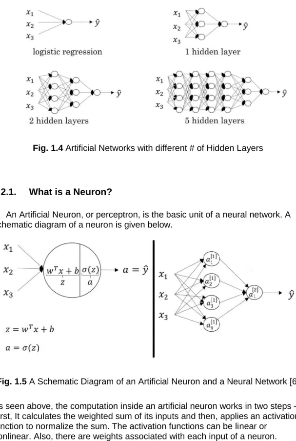
A deep feedforward network is a type of an artificial neural network which connections do not form a cycle, and is the quintessential deep learning model [5]. The purpose of a feedforward network is to approximate a function f∗, based on a defined mapping of an input x to a category y. The best function approximation would be learning which parameters θ of the deep neural network are able to reduce the error between the hypothesis and real output.

In these models, the input x flows through the middle computations in order to define f, and calculate output y. In deep feedforward networks, information flows in one direction, and there are no feedback connections from the output to the input.

A feedforward neural network can consist of three types of layers:

Input Layer: The input nodes provide information from the outside world to the network and are together referred to as the “Input Layer”. No computation is performed in any of the Input nodes – they just pass on the information to the hidden nodes.

Hidden Layer: The hidden nodes have no direct connection with the outside world (hence the name “hidden”). They perform computations and transfer information from the input nodes to the output nodes. A collection of hidden nodes forms a “Hidden Layer”. While a feedforward network will only have a single input layer and a single output layer, it can have zero or multiple Hidden Layers.

If a Neural network has zero hidden layers, it is called a shallow network. On the other hand, if a Neural Network has 1 or multiple hidden layers, it is called a deep network.

Output Layer: The Output nodes are collectively referred to as the “Output Layer” and are responsible for computations and transferring information from the network to the outside world.

Feedforward neural networks are called networks because they are generally represented by linking together many diﬀerent functions. The model is associated with a directed acyclic graph describing how the functions are composed together.

Each function will represent one layer, and the linking of the input and output of each layer is what allows to create one network. The overall length of the chain gives the depth of the model. The name “deep learning” arose from this terminology. The ﬁnal layer of a feedforward network is called the output layer.

A Multi-Layer Perceptron (MLP) contains one or more hidden layers (apart from one input and one output layer). While a single layer perceptron can only learn linear functions, a multi-layer perceptron can also learn non – linear functions, and this is the reason it has more use in real world applications.

(15)

Fig. 1.4 Artificial Networks with different # of Hidden Layers

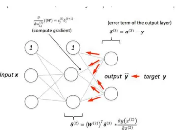
1.2.1. What is a Neuron?

An Artificial Neuron, or perceptron, is the basic unit of a neural network. A schematic diagram of a neuron is given below.

Fig. 1.5 A Schematic Diagram of an Artificial Neuron and a Neural Network [6] As seen above, the computation inside an artificial neuron works in two steps – First, It calculates the weighted sum of its inputs and then, applies an activation function to normalize the sum. The activation functions can be linear or

nonlinear. Also, there are weights associated with each input of a neuron. These are the parameters which the network has to learn during the training phase, in order to calculate better approximations of its output [6].

By having multiple layers, we can compute complex functions by cascading simpler

(16)

1.2.2. Activation Functions

The activation function simulates the behavior of a biological neuron, and is used as a decision making body at the output of a neuron. The neuron learns Linear or Non-linear decision boundaries based on the activation function. It also has a normalizing effect on the neuron output which prevents the output of neurons after several layers to become very large, due to the cascading effect. The most widely used activation functions in artificial neural networks are Sigmoid, Tanh, and Rectified Linear Unit, as shown in the next figure.

Fig. 1.6 Activation functions: Sigmoid, Tanh and ReLU

Overall, the previously mentioned activation functions offer non-linearity which in neural networks allow us to generalize more, and thus calculate better approximations.

The major advantage of Sigmoid and Tanh Activation functions is that they offer a result within a finite boundary, also known as “no blow up activation”. However, the major disadvantage in deep neural networks for these two activations is that the derivative of either one will be less than one.

In Deep Learning, it has been shown that more layers increase performance, but

if you have many layers with these functions, you will multiply these gradients, and the product of many smaller than 1 values goes to zero very quickly. This means that for Deep Learning Sigmoid and Tanh functions are not recommended.

On the other hand, Rectifier Linear Units don’t have the vanishing gradient and also perform less expensive computations, but tend to over fit easily.

In Deep Learning, Rectifier Linear Units are more commonly used, but additional steps need to be done in order to reduce overfitting.

1.2.3. The Back-Propagation Algorithm

The process by which a deep neural network learns is called the Backpropagation algorithm.

(17)

1) A Dataset: consisting of input-output pairs, where is the input and is the desired output of the network on input. The set of input-output pairs of size is denoted.

2) A feedforward neural network, as formally defined concerning feedforward neural networks, whose parameters are collectively denoted. In backpropagation, the parameters of primary interest are, the weight between node in layer and node in layer, and the bias for node in layer. There are no connections between nodes in the same layer and layers are fully connected.

3) An error function, which defines the error between the desired output and the calculated output of the neural network on input for a set of input-output pairs and a particular value of the parameters.

For classification problems, the error function is usually defined using the mean squared error.

𝐸(𝑋) = 1 2𝑁∑ (𝑂𝑖 − 𝑦𝑖) 2 𝑁 𝑖=1 = 1 2𝑁∑ (𝑔(𝑤⃗⃗ ∙ 𝑥𝑖 − 𝑦𝑖) 2 𝑁 𝑖=1 (1.1) Where, 𝐸(𝑋) = Error Function 𝑁 = Number of Layers 𝑂_𝑖 = Estimated Output 𝑦_𝑖 = Real Output

Training a neural network with gradient descent requires the calculation of the gradient of the error function with respect to the weights and biases. Then, according to the learning rate, each iteration of gradient descent updates the weights and biases collectively denoted according to

𝜃𝑡+1_{= 𝜃}𝑡_{− 𝛼}𝜕𝐸(𝑋,𝜃𝑡)

𝜕𝜃 (1.2)

Where,

𝜃 = Parameters of the neural Neural Network

t = iteration in gradient descent

𝛼 = learning rate

This process is repeated until the output error is below a predetermined threshold or minimum.

(18)

Fig. 1.7 A Graphical representation of back propagation of error and weight update.

Initially all the edge weights are randomly assigned. For every input in the training dataset, the ANN is activated and its output is observed. This output is compared with the desired output that we already know, and the error is "propagated" back to the previous layer. This error is noted and the weights are "adjusted" accordingly. This process is repeated until the output error is below a predetermined threshold.

Once the above algorithm terminates, we have a "learned" ANN which, we consider is ready to work with "new" inputs. This ANN is said to have learned from several examples (labeled data) and from its mistakes (error propagation).

In summary, the Backpropagation algorithm goes as follow [8]: 1. Input a set of training examples

2. For each training example 𝑥: Set the corresponding input activation 𝑎𝑥,1, and perform the following steps:

 Feedforward: For each 𝑙=2,3,…,𝐿 compute

𝑧𝑥,𝑙 = 𝑤𝑙𝑎𝑥,𝑙−1+ 𝑏𝑙And 𝑎𝑥,𝑙−1 = 𝜎(𝑧𝑥,𝑙−1)

 Output error𝛿𝑥,𝐿_{: Compute the vector}

(19)

3. Gradient descent: For each 𝐿=L,L-1,…,2 update the weights according to the rule 𝑤𝑙 → 𝑤𝑙− 𝑛

𝑚∑ 𝛿

𝑥,𝑙_(𝑎𝑥,𝑙−1₎𝑇

𝑥 , and the biases according to the rule

𝑏

𝑙

→ 𝑏

𝑙

−

𝑛

𝑚

∑ 𝛿

𝑥,𝑙 𝑥 .

To implement in practice you also need an outer loop generating mini-batches of training examples, and an outer loop stepping through multiple epochs of training.

1.3. Deep Learning Architectures

The number of architectures and algorithms that are used in deep learning is wide and varied. This section explores five of the deep learning architectures spanning the past 20 years. Notably, LSTM and CNN are two of the oldest approaches in this list but also two of the most used in various applications[9].

Fig. 1.8 Deep Learning Applications

These architectures are applied in a wide range of scenarios, but the following table lists some of their typical applications.

Architecture Application

RNN Speech recognition, handwriting recognition

LSTM/GRU networks

Natural language text compression, handwriting recognition, speech recognition, gesture recognition, image captioning

CNN Image recognition, video analysis, natural language

processing

DBN Image recognition, information retrieval, natural language

(20)

As we can see from the table above, the recommended architecture for video analysis and image recognition is Convolutional Neural Networks.

We will explain ConvNets in more detail in the following chapter.

(21)

Chapter 2 CONVOLUTIONAL NEURAL NETWORKS

In Deep Learning, a convolution neural network (CNN, or ConvNet) is a class of a deep feed-forward network that makes the explicit assumption that the inputs are images, which allows us to define certain properties into the architecture. These then make the computation functions more efficient to implement and reduce the amount of parameters in the network. Due to this, they have been successfully applied to visual imagery analysis, and have applications in image and video classification.

2.1. Architecture Overview

Convolutional Neural Networks are very similar to ordinary Neural Networks from the previous chapter: they are made up of neurons that have learnable weights and biases. Each neuron receives some inputs, performs a dot product and optionally follows it with a non-linearity. The whole network still expresses a single differentiable score function: from the raw image pixels on one end to class scores at the other. And they still have a loss function) on the last (fully-connected) layer.

However, unlike other neural networks, Convolutional Neural Networks take advantage of the fact that the input consists of images and they constrain the architecture in a more sensible way. In particular, the layers of a ConvNet have neurons arranged in 3 dimensions: width, height, depth.

In images, this translates to pixel height, width, and rgb channels.

Fig. 2.1 A regular 3-Layer NN vs a ConvNet[11]

As we described above, a simple ConvNet is a sequence of layers, and every layer of a ConvNet transforms one volume of activations to another through a differentiable function. We use three main types of layers to build ConvNet architectures: Convolutional Layer, Pooling Layer, and Fully-Connected Layer (exactly as seen in regular Neural Networks).

(22)

2.1.1. Convolutional Layer

The Conv layer is the core building block of a Convolutional Network that does most of the computational heavy lifting.

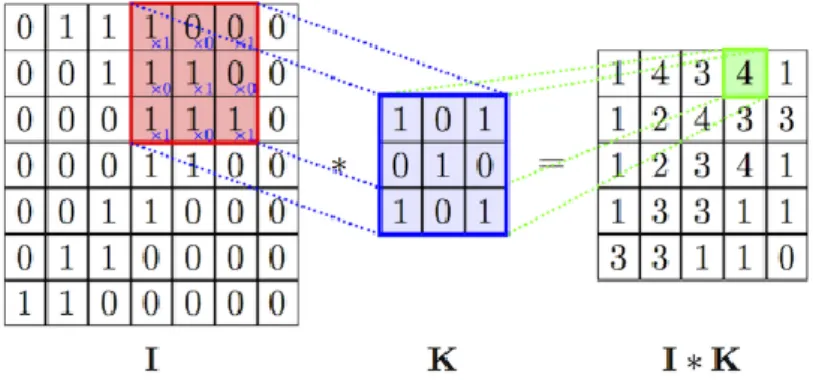
Convolution is a mathematical operation that basically takes two functions (f and g) to produce a third one (f*g).

In the context of CNN, a Convolution is the treatment of a matrix by another called kernel. This has been applied in image processing before the creation of CNN.

The convolutional process in a convolutional goes as follows: the kernel is moving in the input, from left to right and from top to bottom, and each one of the values on the kernel is multiplied by the value on the input on the same position. The results obtained by the multiplication are then summed and the local output is generated.

Fig. 2.2 A Convolutional Operational between an Input and Kernel

The main task of the convolutional layer is to extract features from the previous layer and mapping their appearance to a feature map. As a result of convolution in neural networks, the image is split into perceptrons, creating local receptive fields and finally compressing the perceptrons in feature maps. Convolution preserves the spatial relationship between pixels by learning image features using small squares of input data. Hence, each filter is trained spatial in regard to the position in the volume it is applied to.

The output volume of a convolutional layer is defined by four hyperparameters:  Number of Filters or Depth (K): Defines how many features the layer will

detect.

 Filter Size or Depth (F): Defines the feature activation area of each filter.  Stride(S): which defines the movement or slide of a kernel through the

input,

 Zero Padding (P): control the spatial size of the output volumes

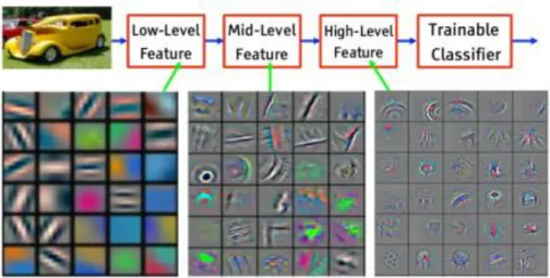
The result of staging these convolutional layers in conjunction with the following layers is that the information of the image is classified like in vision. That means that the pixels are assembled into edges, edges into motifs, motifs into parts,

(23)

parts into objects, and objects into scenes. This effect is observable in the appearance of the filters and shown in the next figure [12].

Fig. 2.3Feature learning in a Convolutional Neural Network

2.1.2. Pooling Layer

The pooling or down sampling layer is responsible for reducing the spacial size of the activation maps. In general, they are used after multiple stages of other layers (i.e. convolutional and non-linearity layers) in order to reduce the

computational requirements progressively through the network as well as minimizing the likelihood of overfitting.

The output volume of a pooling layer is defined by two hyperparameters:  Filter Size or Depth (F)

 Stride(S)

The definition for Filter Size and Stride in the pooling layer is the same as in the convolutional layers

The pooling layer operates by defining a window of size F(l)×F(l) and reducing the data within this window to a single value. The window is moved

by S(l) positions after each operation similarly to the convolutional layer and the reduction is repeated at each position of the window until the entire activation volume is spatially reduced.

(24)

Fig. 2.4 Pooling Example of a 224x224 Image

The most common methods for reduction are max pooling and average pooling. Max pooling operates by finding the highest value within the window region and discarding the rest of the values. Average pooling on the other hand uses the mean of the values within the region instead.

Max pooling has demonstrated faster convergence and better performance in comparison to the average pooling and other variants such as l2l2-norm pooling (9). Thus, recent work generally trends towards max pooling or similar variants.

Fig. 2.5 Max Pool Operation on a 4x4 Input

2.1.3. Rectified Linear Units (ReLUs)

The rectified linear units (ReLUs), already explained in chapter 1, are the default activation function in neural network. As a result of its advantages and performance, most of the recent architectures of convolutional neural networks utilize only rectified linear unit layers (or its derivatives such as noisy or leaky ReLUs) as their non-linearity layers instead of traditional non-linearity and rectification layers. In works such as AlexNet[7]rectified linear units are shown to operate six times faster then hyperbolic tangent non-linearities while reaching 25% error rate on CIFAR-10 datase). More recently, utilization of an advanced derivative Parametric Rectified Linear Units (PReLU) allowed convolutional networks to surpass human-level performance in ImageNet database ).

(25)

2.1.4. Fully Connected Layer

The fully connected layers in a convolutional network are practically a multilayer perceptron (generally a two or three layer MLP) that aims to map

the m1(l−1)×m2(l−1)×m3(l−1) activation volume from the combination of previous different layers into a class probability distribution. Thus, the output layer of the multilayer perceptron will have m(l−i)1m1(l−i) outputs, i.e. output neurons where ii denotes the number of layers in the multilayer perceptron. The purpose of a fully connected layer in a convolutional network is the same as other deep feedforward networks, to be able to classify more complex functions. The key difference from a standard multilayer perceptron is the input layer where instead of a vector, an activation volume (from the previous convolutional layers) is taken as an input.

Fig. 2.6A Fully Connected Neural Network

2.1.5. Softmax Layer

The softmax function squashes the outputs of each unit to be between 0 and 1, just like a sigmoid function. But it also divides each output such that the total sum of the outputs is equal to 1 (check it on the figure above).

Fig. 2.7Softmax Operation Example

The output of the softmax function is equivalent to a categorical probability distribution, it tells you the probability that any of the classes are true, which

(26)

makes it suitable for classification problems using convolutional neural

networks. Please note that the softmax layer is reserved for the output layer of a convolutional network.

Mathematically the softmax function is shown below, where z is a vector of the inputs to the output layer (if you have 10 output units, then there are 10 elements in z). And again, j indexes the output units, so j = 1, 2,....K.

𝜎(𝑧)

_𝑗

=

𝑒𝑧𝑗

∑𝐾_𝑘=1𝑒𝑧𝑘

(2.1)

2.1.6. A Convolutional Network – Stacking the Layers

In a simple Convolutional Network Architecture, these layers are stacked together: INPUT - CONV - RELU - POOL – FC

The general description of the each layer is as follows:

 INPUT [32x32x3] will hold the raw pixel values of the image, in this case an image of width 32, height 32, and with three color channels R,G,B.

 CONV layer will compute the output of neurons that are connected to local regions in the input, each computing a dot product between their weights and a small region they are connected to in the input volume. This may result in volume such as [32x32x12] if we decided to use 12 filters.

 RELU layer will apply an element wise activation function, such as the max(0,x)max(0,x) thresholding at zero. This leaves the size of the volume unchanged ([32x32x12]).

 POOL layer will perform a down sampling operation along the spatial dimensions (width, height), resulting in volume such as [16x16x12].

 FC (i.e. fully-connected) layer will compute the class scores, resulting in volume of size [1x1x10], where each of the 10 numbers correspond to a class score, such as among the 10 categories of CIFAR-10. As with ordinary Neural Networks and as the name implies, each neuron in this layer will be connected to all the numbers in the previous volume.

2.2. Convolutional Neural Network Architectures

Deep neural networks and Deep Learning are powerful and popular algorithms. And a lot of their success lays in the careful design of the neural network

architecture.

We have seen that Convolutional Networks are commonly made up of only three layer types: CONV, POOL (we assume Max pool unless stated otherwise) and FC (short for fully-connected). We will also explicitly write the RELU activation function as a layer, which applies element wise non-linearity. In this section we discuss how these are commonly stacked together to form entire ConvNets.

(27)

2.2.1. Layer Patterns

The most common form of a ConvNet architecture stacks a few CONV-RELU layers, follows them with POOL layers, and repeats this pattern until the image has been merged spatially to a small size. At some point, it is common to transition to fully-connected layers. The last fully-connected layer holds the output, such as the class scores. In other words, the most common ConvNet architecture follows the pattern:

INPUT -> [[CONV -> RELU]*N -> POOL?]*M -> [FC -> RELU]*K -> FC

where the * indicates repetition, and the POOL? indicates an optional pooling layer. Moreover, N >= 0 (and usually N <= 3), M >= 0, K >= 0 (and usually K

< 3).

For example, here are some common ConvNet architectures you may see that follow this pattern:

 INPUT -> FC, implements a linear classifier. Here N = M = K = 0.

 INPUT -> CONV -> RELU -> FC

 INPUT -> [CONV -> RELU -> POOL]*2 -> FC -> RELU -> FC. Here we see that there is a single CONV layer between every POOL layer.

 INPUT > [CONV > RELU > CONV > RELU > POOL]*3 > [FC -> RELU]*2 --> FC Here we see two CONV layers stacked before every POOL layer. This is generally a good idea for larger and deeper networks, because multiple stacked CONV layers can develop more complex features of the input volume before the destructive pooling operation.

It should be noted that the conventional paradigm of a linear list of layers has recently been challenged, in Google’s Inception [13] architectures and also in current (state of the art) Residual Networks from Microsoft Research Asia. Both of these (see details below in case studies section) feature more intricate and different connectivity structures.

It is recommended thatinstead of rolling your own architecture for a problem, you should look at whatever architecture currently works best on ImageNet, download a pretrained model and finetune it on your data. You should rarely ever have to train a ConvNet from scratch or design one from scratch.

2.2.2. Case Studies

There are several architectures in the field of Convolutional Networks that have a name. The most common are:

 LeNet. The first successful applications of Convolutional Networks were developed by Yann LeCun in 1990’s. Of these, the best known is

the LeNet architecture that was used to read zip codes, digits, etc.

 AlexNet[7]. The first work that popularized Convolutional Networks in Computer Vision was the AlexNet, developed by Alex Krizhevsky, Ilya

(28)

Sutskever and Geoff Hinton. The AlexNet was submitted to the ImageNet ILSVRC challenge in 2012 and significantly outperformed the second runner-up (top 5 error of 16% compared to runner-runner-up with 26% error). The Network had a very similar architecture to LeNet, but was deeper, bigger, and

featured Convolutional Layers stacked on top of each other (previously it was common to only have a single CONV layer always immediately followed by a POOL layer).

 ZF Net. The ILSVRC 2013 winner was a Convolutional Network from Matthew Zeiler and Rob Fergus. It became known as the ZFNet (short for Zeiler & Fergus Net). It was an improvement on AlexNet by tweaking the architecture hyperparameters, in particular by expanding the size of the middle convolutional layers and making the stride and filter size on the first layer smaller.

 GoogLeNet.[13] The ILSVRC 2014 winner was a Convolutional Network from Szegedy et al. from Google. Its main contribution was the development of an Inception Module that dramatically reduced the number of parameters in the network (4M, compared to AlexNet with 60M). Additionally, this paper uses Average Pooling instead of Fully Connected layers at the top of the ConvNet, eliminating a large amount of parameters that do not seem to matter much. There are also several followup versions to the GoogLeNet, most recently Inception-v4.

 VGGNet. The runner-up in ILSVRC 2014 was the network from Karen Simonyan and Andrew Zisserman that became known as the VGGNet. Its main contribution was in showing that the depth of the network is a critical component for good performance. Their final best network contains 16 CONV/FC layers and, appealingly, features an extremely homogeneous architecture that only performs 3x3 convolutions and 2x2 pooling from the beginning to the end. Their pretrained model is available for plug and play use in Caffe. A downside of the VGGNet is that it is more expensive to

evaluate and uses a lot more memory and parameters (140M). Most of these parameters are in the first fully connected layer, and it was since found that these FC layers can be removed with no performance downgrade,

significantly reducing the number of necessary parameters.

 ResNet[14]. Residual Network developed by Kaiming He et al. was the winner of ILSVRC 2015. It features special skip connections and a heavy use of batch normalization. The architecture is also missing fully connected layers at the end of the network. ResNets are currently by far state of the art Convolutional Neural Network models and are the default choice for using ConvNets in practice (as of May 10, 2016). In particular, also see more recent developments that tweak the original architecture from Kaiming He et al. Identity Mappings in Deep Residual Networks (published March 2016). The following figure summarizes the performance of different ConvNet

(29)

(30)

Chapter 3 TESTING AND RESULTS

This chapter explains one possible implementation of automatic video classification. The goal is to have a proof of concept of implementing an automatic flagging of adult video content using Deep Learning.

Throughout this chapter, you will find a general description of the architecture of the solution, the methodology followed, the dataset used, how the solution was implemented, and the results achieved.

This chapter is a starting point for developing an adult content video classifier focused on nudity and/or pornographic content, but could be extended to include gory or graphic content not suitable for minors (narcotics use or violence, for example).

The system described here is capable of classifying a video into two classes: 1. Not Safe for Work

2. Safe for Work

The proposal to solve this problem is an architecture based on convolutional neural networks

.

3.1. Description of the Architecture of the Solution

Video has the distinct property that it includes spatial information (in images) and temporal information (context of each frame relative with other frames in time). We hypothesize that since video is a combination of single frames (or images), the correct classification of single images should translate to a correct classification of a video stream with high accuracy.

The neural network is a convolutional neural network with the purpose of extracting high-level features of the images and reducing the complexity of the input. Using the convolutional neural network, we will classify an image into safe for work (Safe for work) or suitable for all audiences, or Not Safe for Work (adult content).

For the convolutional neural network of the solution, we will be using a pre-trained model called Open NSFW [15] developed by Yahoo.

From the Yahoo Open NSFW Git Hub site[16], the usage of the OPEN NSFW is as follows:

 The network takes in an image and gives output a probability (score between 0-1) which can be used to filter not suitable for work images. Scores < 0.2 indicate that the image is likely to be safe with high

(31)

probability. Scores > 0.8 indicate that the image is highly probable to be NSFW. Scores in middle range may be binned for different NSFW levels.

Figure 3.1 SFW image classification examples using OPEN NSFW[16]

Open NSFW is a convolutional neural network based on the thin resnet 50 1by2 architecture, which is a less computational demanding model based on the ResNet Model, and was pre trained on the ImageNet 1000 class dataset.

Fig. 3.1 Graph of the Residual Network Model

We used this model to apply the technique of transfer learning. Modern object recognition models have millions of parameters and can take weeks to fully train. Transfer learning is a technique that optimizes a lot of this work by taking a fully trained model for a set of categories like ImageNet and retrains from the existing weights for new classes.

For video classification, several approaches can be used over single or multi frame analysis. According to a Google research paper , Large-scale Video Classification with Convolutional Neural Networks[17]” Our best spatio-temporal networks display significant performance improvements compared to strong feature-based baselines (55.3% to 63.9%), but only a surprisingly modest improvement compared to single-frame models (59.3% to 60.9%).”

(32)

Figure 3.2Figure from Google's research paper explaining different approaches for video analysis using convolution neural networks.

Having that said, in order to reduce complexity on the proposed solution, we will evaluate the video classifier based on a single frame classification and evaluate its performance.

3.2. Methodology

The first step is to extract the frames of the video. We extract a frame of the video and using this frame, we make a prediction using the open nsfw. We will continue this process until the end of video is reached.

During each iteration, what we see on the screen is a classification of the video in real-time — either safe, or not safe for work.

Fig. 3.2 NSFW Video Classification Methodology

After getting the classification of each frame, the max score will be stored for the video. After the end of the video, if the max score is greater than 0.8, the video will be flagged as Not safe for Work.

(33)

3.3.1. The Dataset

In order to assess the open nsfw network accuracy performance, we will use the dataset used in the research paper “Nude Detection in Video using Bag-of-Visual-Features” [19]. This dataset was selected due to its similarity in adult video scenarios seen on TV and other video content platforms.

Figure 3.3 Examples of Non-Nude (Top) and Nude (Bottom) Frames from the dataset.

The description of the dataset goes as follows:

The database of nude and non-nude videos contains a collection of 179 video segments collected from the following movies: Alpha Dog, Basic Instinct, Before The Devil Knows You're Dead, Cashback, Eros, Les Anges Exterminateurs, Loner, Original Sin, Primer, Striptease and The Bubble. For nude samples, longer sequences were partitioned into shorter ones. The sequences for the non-nude class were collected by randomly selecting the initial time and length. Random selections which felt inside a nude scene were discarded. Those random selections were performed on the same movies above listed for the nude class.

A summary of the database.

Class Segments Seconds

Non-Nude 90 506

Nude 89 589

All 179 1095

Number of video segments per video.

Video Name #Non-Nude #Nude

Alpha Dog 10 07

Basic Instinct 10 15

Before The Devil Knows You're Dead 10 06

Cashback 10 10

Eros - 16

Les Anges Exterminateurs 10 18

(34)

Original Sin 10 04

Primer 10 -

Striptease - 11

The Bubble 10 02

3.3.2. Performance Metrics

For the purpose of this thesis, a nude video segment should be flagged as Not-Work (NSFW), and a non-nude video should be flagged as Safe-for-Work (SFW).

In order to assess the proposed solution’s performance, we will draw its confusion matrix based on this dataset, and calculate its related metrics based on confusion matrix analysis.

The confusion matrix is simply a square matrix that reports the counts of the true positive (TP), true negative (TN), false positive (FP), and false negative (FN)

predictions of a classifier, as shown in the following figure:

Figure 3.4 Confusion Matrix

Since our classification solution only has two classes: NSFW and SFW, we can, alternatively, view the confusion matrix as follows

(35)

From the figure above, the acronym TP, FN, FP, and TN of the confusion matrix cells refers to the following:

TP = true positive, the number of NSFW Videos that are correctly identified as NSFW. FN = false negative, the number of NSFW Videos that are misclassified as SFW. FP = false positive, the number of SFW Videos that are incorrectly identified as NSFW. TN = true negative, the number of SFW Videos that are correctly identified as SFW.

The performance of the solution will be measured on the following metrics [19]:  Accuracy: Assesses the overall effectiveness of the algorithm by

estimating the probability of the true value of the class label. Ideal Value: Probability of 100%.

𝐴𝑐𝑐𝑢𝑟𝑎𝑐𝑦 = 𝑇𝑃+𝑇𝑁

𝐹𝑃+𝐹𝑁+𝑇𝑁+𝑇𝑃 (3.1)

 Error Rate: 1- Accuracy. Is an estimation of misclassification probability according to model prediction.

Ideal Value: Probability of 0%.

𝐸𝑟𝑟𝑜𝑟 𝑅𝑎𝑡𝑒 = 1 − 𝐴𝑐𝑐𝑢𝑟𝑎𝑐𝑦 = 𝐹𝑃+𝐹𝑁

𝐹𝑃+𝐹𝑁+𝑇𝑁+𝑇𝑃 (3.2)  Sensitivity or Recall: True Positive Rate. Estimates the proportion of positives that are correctly identified as such. It gives a value for the probability of detection.

Ideal Value: Coefficient of 1

𝑅𝑒𝑐𝑎𝑙𝑙(𝑅𝐸𝐶) = 𝑇𝑃

𝑇𝑃+𝐹𝑁 (3.3)

 Specificity: True Negative Rate. Estimates the proportion of negatives that are correctly identified as such.

𝑆𝑝𝑒𝑐𝑖𝑓𝑖𝑐𝑖𝑡𝑦 = 𝑇𝑁

𝑇𝑁+𝐹𝑃 (3.4)

 Precision: It is the ratio of true positives compared to the total number of positives predicted by the model. It gives an estimate of the confidence we can have in the predicted value.

𝑃𝑟𝑒𝑐𝑖𝑠𝑖𝑜𝑛 (𝑃𝑅𝐸) = 𝑇𝑃

𝑇𝑃+𝐹𝑃 (3.5)

 F1 Score: Combines the values of Precision and Recall to give an assessment over a single metric. Since Precision and Recall give complementary information, it is used to give a general overview of a model’s performance over true classes.

(36)

𝐹1 𝑆𝑐𝑜𝑟𝑒 = 2𝑅𝐸𝐶+𝑃𝑅𝐸

𝑅𝐸𝐶∗𝑃𝑅𝐸 (3.6)

 MCC: MCC Matthew’s correlation coefficient is a single performance

measure less influenced by imbalanced test sets since it considers mutually accuracies and error rates on both classes, and involve all values of confusion matrix. It is considered to be the best single assessment metric in a model’s prediction performance.

Ideal Value: MCC ranges from 1 for a perfect prediction to-1 for the worst possible prediction. MCC close to 0 indicate a model that performs randomly.

𝑀𝐶𝐶 = 𝑇𝑃𝑥𝑇𝑁−𝐹𝑃𝑥𝐹𝑁

√(𝑇𝑃+𝐹𝑃)(𝑇𝑃+𝐹𝑁)(𝑇𝑁+𝐹𝑃)(𝑇𝑁+𝐹𝑁) (3.7)

3.4. Implementation

The solution for the adult content classifier was implemented with Python 3.5. We use OpenCV and Tensorflow for Python to segment the video in frames. Once we have a frame, we make a prediction using the open nsfw model using each of them.

The result of each prediction is a “transfer value” representing the high-level feature map extracted from that specific frame. We continue this process until the end of video is reached.

(37)

The OPEN NSFW Video Classifier is composed of the following parts:

1. Video application Code: Analyzes each frame through the open nsfw model continuously until video ends.

2. ResNet Model: Based on the Thin ResNet 50-1by2 used by Open NSFW from Yahoo, classifies each frame into NSFW or SFW. 3. Image Loader: Converts an image so it can be loaded to the open

nsfw model.

4. Model Weights: Data of the weight parameters in the open nsfw already pretained by Yahoo.

You can see the complete implementation code in annex [B].

3.5. Results

This sections shows the results for video classification based on the open nsfw +video solution for three common scenarios in video found on television programs and video content platforms over the Internet. After defining the classification method for each type of video, we will review the results with the proposed dataset, and calculate the performance metrics as proposed in the previous section 3.3.2

It is important to mention that, as in any deep learning model, we will have scenarios were an object is misclassified since the model’s performance will never be 100% accurate all the time. Having that said, we will review the misclassification examples of each type of video as well.

We will perform the test on the following type of videos:

- Safe for Work: Suitable for all audiences, shown during 0600 – 1800 timeslot. Safe for Work videos should be classified SFW during their entire run time.

- Not Safe for Work: Suitable for adults audiences, shown during 1800-0400 Not Safe for Work videos should be classified NSFW during portions of their entire run time.

- Safe for work +, Suitable for teenagers and adult audiences, shown during 1800-0600. Safe for Work+ videos should be classified SFW during their entire run time. There will be portions of SFW+ videos with edge scenarios, NSFW in the 0.5-0.8 range. These type of videos should be combine human moderation with the machine learned solution to improve performance.

3.5.1. SFW: A cartoon video: “Big Buck Bunny” (2007)

This video is a cartoon film released in 2007, and we will use as an example of video shown to children in television during the AM runtime.

(38)

SFW video: Big Buck Bunny: Safe for Work. Classification: Correct, SFW

Figure 3.7 SFW classification for a SFW Video, 3 consecutive frames shown with NSFW score: 0.0683, 0.1593, and 0195, respectively

SFW video: Big Buck Bunny: Safe for Work. Classification: Incorrect, NSFW

Figure 3.8 NSFW classification for a SFW Video, 3 consecutive frames shown with NSFW score: 0.8231, 0.9220, and 0.8805, respectively

3.5.2. NSFW: An adult TV show video: “Game of Thrones” (2011-Present).

This video is from the HBO Game of Thrones TV show, which is famous for having sex and violent scenes on television, and we will use as an example of video shown targeted to adult audiences in television during the PM run time. These type of videos should be classified as NSFW during some portions of their run time.

NSFW video: Game of thrones: Safe for Work portion. Classification: Correct, SFW

Figure 3.9 SFW classification for a SFW portion from a NSFW Video,1 frame shown with NSFW score: 0.0358

NSFW video: Game of thrones: Not Safe for Work portion. Classification: Correct, NSFW

(39)

Figure 3.10 NSFW classification for a NSFW Video, NSFW portion 3 consecutive frames shown with NSFW score: 0.9632, 0.9510, and 0.9572,

respectively.

NSFW video: Game of thrones: Not Safe for Work portion. Classification: Incorrect, SFW

Figure 3.11 SFW classification for a NSFW portion from a NSFW video, 1 frame shown with 0.1171.

3.5.3. SFW+: Teen and Adult TV show video: “Miss Universe Bikini” (2011).

This video is from the Miss Universe Pageant TV show, which is famous for having beautiful women modelling and posing with bikinis on television, and we will use as an example of video shown targeted to teen and adult audiences in television during the PM run time.

SFW video: Miss Universe Bikini Competition. Classification: Correct, SFW

Figure 3.12 SFW classification from a SFW+ video, 2 frames shown with NSFW scores: 0.2795 and 0.2129.

(40)

SFW+ video: Miss Universe Bikini Competition. Classification: Correct, SFW

Figure 3.13 SFW classification from a SFW+ video, 3 frames shown with NSFW scores: 0.3301, 0.3238, and 0.3868.

The above figures shows a correct classification of SFW content, in a hard-to-detect scenario for nudity.

However, the following figure will show that, even though the solution classifies correctly most of the scenarios, some errors in classification will occur. In this particular scenario, three frames have been tagged NSFW with high confidence. SFW+ video: Miss Universe Bikini Competition.

Classification: Incorrect, NSFW

Figure 3.14 NSFW classification from a SFW+ video, 3 frames shown with NSFW scores: 0.9871, 0.9837, and 0.9895

3.5.4. Performance Metrics Results for OPEN NSFW Video

After defining how the classification of each video was performed, we plot the results in the following confusion matrix using the dataset proposed in section 3.3.1:

Note: Please find the results for each segment of the video in Annex [A].

(41)

Figure 3.15 Confusion Matrix for Open NSFW Video

Classification of the Dataset Number of Segments

Summary

True Positive = NSFW + NSFW Tag 68 TP False Negative = NSFW + SFW Tag 21 FN False Positive = SFW + NSFW Tag 12 FP True Negative = SFW + SFW Tag 78 TN

Total 179

We can calculate the performance metrics of the proposed open nsfw video solution, using the formulas proposed in section 3.3.2:

Fundamental Evaluation Measures Value

Accuracy 0.816

Error Rate 0.184

Sensitivity or Recall (True Positive Rate)

0.764

Specificity (True Negative Rate) 0.867

Precision 0.850

Combined Evaluation Measures Value

F1-Score 0.8047

MCC 0.6343

As previously mentioned, a F1-Score close to 1 and a MCC greater 0 indicate that model performs better than a random guessing model.

(42)

Chapter 4 Conclusions

This chapter presents the conclusions and possible future improvements of the Project presented in this master thesis.

4.1. Conclusions and Results

This master thesis final project has been motivated by the growing consumption of video content over the past years. Additionally, this increase in video consumption has led to an increase in adult video content which might be offensive or not suitable for minors. Given the amount of new video content that is reachable in the public domain, there is an urgent need to isolate adult videos

from non-offensive ones without manual intervention.

In previous approaches of machine learning, intelligent analysis of video would require a manual engineering of features to be able to detect offensive video. However, as explained, in chapter 1 a new paradigm in machine learning called deep learning has allowed us to overcome this deficiency and use end-to-end approaches using data only, to improve neural networks learning.

We propose to build an offensive video classifier based on one of the recently flourishing deep learning techniques. The most remarkable thing about deep neural networks is that no human programming is needed to be able to learn correct classification. In image classification, convolutional neural networks contain many layers for both automatic features extraction and classification. The benefit is an easier system to build and improve through time, since we remove the previous approach of manual feature engineering.

In order to assess the proposed solution’s performance, we used a standard approach by using a confusion matrix and calculating the performance model’s metrics. From the results, we can confirm the proposed model has an acceptable performance but could be improved using various techniques. Additionally, the performance metrics give valuable insights on what results can be expected using single-frame approaches in video analysis. Lastly, the proposed solution can also work as a benchmark for classifying offensive video using deep neural networks.

4.2. Future Work Lines

In terms of future improvements, it is desirable to run the model in an extended dataset, in order to verify the efficiency of the algorithm and to make further improvements. Although the algorithm is efficient, an evaluation of other data sets would confirm that the model does not over fit to our dataset, which would give a false sense of a good performance.

Secondly, as in any deep learning project, we could further improve the open nsfw model by retraining the current open nsfw model through hyper parameter

(43)

tuning, data augmentation. Using this methods, we could confirm if the values used in the current model are the giving the best performance for this type of classification.

Another further improvement of the algorithm would be to include the temporal information found in video to the current solution, since we only used a single-frame analysis for the dataset. It is suggested in Google’s research paper that including a slow-fusion approach could increase the performance of the video analyzer by 1%. A next line of work would be to add the temporal analysis using a long-short term memory network and compare the results with the current network.

Additionally, after improving the open nsfw classifier, we could also develop another nsfw classifier using another convolutional network architecture such as Google’s Inception Network or another type of ResNet. Google’s Inception Network is already included in the tensorflow framework and could be retrained to classify nsfw images. After building the new nsfw classifier, we could use the same dataset and compare the performance of both solutions.

Lastly, after building and comparing different models, we could create an ensemble network by combining the performance of all networks into a single network. If the performance is better than human classification, it could be used as a commercial application for adult video detection in a television network or a video content provider.

(44)

Abbreviations and Acronyms

Acronym Name

AI Artificial Intelligence ANN Artificial Neural Network

CDBN Convolutional Deep Belief Networks CNN Convolutional Neural Network ConvNet Convolutional Neural Network DBN Deep Belief Network

DeconvNet DeConvolutional Neural Network DL Deep Learning

DNN Deep Neural Network FC Fully Connected

FCN Fully Convolutional Network

FC-CNN Fully Convolutional Convolutional Neural Network ML Machine Learning

MLP Multi-Layer Perceptron NN Neural Network

NSFW Not Safe for Work ReLU Rectified Linear Unit SFW Safe for Work

(45)

Bibliography

[1] Gibson, A. and Patterson, J. “A Review of Machine Learning”, Chap. 1 in

Deep Learning: A Practitioner’s Approach, O'Reilly (2017).

[2] Nielsen, M.A, “Using neural nets to recognize handwritten digits”, Chap. 1 in Neural Networks and Deep Learning, Determination Press (2015). [3] Andrew Ng, “Why deep learning”, Slide 30 in What Data Scientists

Should Know about Deep Learning, Extract Data Conference (2015). https://www.slideshare.net/ExtractConf/andrew-ng-chief-scientist-at-baidu [4] Shaikh F., Deep Learning vs. Machine Learning – the essential

differences you need to know! (2017)

https://www.analyticsvidhya.com/blog/2017/04/comparison-between-deep-learning-machine-learning/

[5] Goodfellow I. et al, “Deep Feedforward Networks”, Chap. 6 in Deep Learning, pg. 168-169,MIT Press (2016)

[6] Aggarwal C., “Neural Networks: A Review”, Chap. 8 in Data Classifications and Algorithms, pg. 209, CRC Press (2014)

[7] Krizhevsky A. et al, “ImageNet classification with deep convolutional

neural networks” in Advances in neural information processing systems,

pg. 1097-1105,(2012)

[8] Nielsen, M.A, “How the backpropagation algorithm works”, Chap. 2 in

Neural Networks and Deep Learning, Determination Press (2015).

[9] Jones. T , “Deep Learning Architectures” in Deep Learning Architectures, IBM Corporation (2017)

https://www.ibm.com/developerworks/library/cc-machine-learning-deep- learning-architectures/cc-machine-learning-deep-learning-architectures-pdf.pdf

[10] Srinivas S et al “A Taxonomy of Deep Convolutional Neural Nets for

Computer Vision”in Front. Robot. AI (2016)

https://doi.org/10.3389/frobt.2015.00036

[11] Karpathy A. “Convolutional Neural Networks (CNNs / ConvNets)” in

Convolutional Neural Networks in Visual Recognition Lecture, Stanford (2016)

[12] Zeiler M. et al, “Deconvolutional Networks” in In CVPR, IEEE (2010) [13] Szegedy C. et al, “Going Deeper with Convolutions” in CVPR 2015,

(46)

[14] He K. et al, “Deep Residual Learning for Image Recognition” in CVPR 2016, Microsoft Research (2015)

[15] Mahadeokar J. et al, “Open sourcing a deep learning solution for nsfw

images”, Yahoo (2016)

https://yahooeng.tumblr.com/post/151148689421/open-sourcing-a-deep-learning-solution-for

[16] Mahadeokar J. et al “Open nsfw model” in Open NSFW github repository (2015) https://github.com/yahoo/open_nsfw

[17]A Karpathy et al “Large-scale Video Classification with Convolutional

Neural Networks” in CVPR 2014, IEEE (2014)

[18] LOPES, A. et al “Nude Detection in Video using Bag-of-Visual-Features”. In: 22th Brazilian Symposium on Computer Graphics and Image (SIBGRAPI), Rio de Janeiro, RJ, 2009

[19] Bekkar M. et al, “Fundamental evaluation measures” Chapter 2 in

Evaluation Measures for Models Assessment over Imbalanced Data Sets

in Vol.3, No.10, 2013. 27, in Journal of Information and Engineering Applications (2013).

(47)

Annex

Annex [A]: Evaluation Results for each video segment using OPEN NSFW video

N. Type Movie Segment Evaluation Max Score NSFWPrediction

1 Nude AlphaDog 1 NSFW 0.9684 Correct

2 Nude AlphaDog 2 SFW 0.4859 Incorrect

7 Nude AlphaDog 7 SFW 0.6827 Incorrect

8 Nude BasicInstinct 1 NSFW 0.9462 Correct

9 Nude BasicInstinct 2 SFW 0.7826 Incorrect

17 Nude BasicInstinct 10 SFW 0.2322 Incorrect 18 Nude BasicInstinct 11 SFW 0.2646 Incorrect

23 Nude BeforeTheDevilKnows 1 SFW 0.0117 Incorrect 24 Nude BeforeTheDevilKnows 2 NSFW 0.8148 Correct 25 Nude BeforeTheDevilKnows 3 NSFW 0.9491 Correct 26 Nude BeforeTheDevilKnows 4 NSFW 0.9061 Correct 27 Nude BeforeTheDevilKnows 5 NSFW 0.9953 Correct 28 Nude BeforeTheDevilKnows 6 NSFW 0.9998 Correct

29 Nude Cashback 1 SFW 0.0491 Incorrect

31 Nude Cashback 3 NSFW 0.8713 Correct

39 Nude Eros 1 NSFW 0.9911 Correct

42 Nude Eros 4 SFW 0.6227 Incorrect