A MapReduce-based distributed SVM algorithm for automatic image annotation

Contents lists available atSciVerse ScienceDirect

Computers and Mathematics with Applications

journal homepage:www.elsevier.com/locate/camwa

A MapReduce-based distributed SVM algorithm for automatic image

annotation

Nasullah Khalid Alham, Maozhen Li

∗

, Yang Liu, Suhel Hammoud

School of Engineering and Design, Brunel University, Uxbridge, Middlesex, UB8 3PH, UK

a r t i c l e i n f o

Keywords:

Automatic image annotation MapReduce framework Sequential minimal optimization Support vector machine

a b s t r a c t

Machine learning techniques have facilitated image retrieval by automatically classifying and annotating images with keywords. Among them Support Vector Machines (SVMs) have been used extensively due to their generalization properties. However, SVM training is notably a computationally intensive process especially when the training dataset is large. This paper presents MRSMO, a MapReduce based distributed SVM algorithm for automatic image annotation. The performance of the MRSMO algorithm is evaluated in an experimental environment. By partitioning the training dataset into smaller subsets and optimizing the partitioned subsets across a cluster of computers, the MRSMO algorithm reduces the training time significantly while maintaining a high level of accuracy in both binary and multiclass classifications.

©2011 Elsevier Ltd. All rights reserved.

1. Introduction

The increasing number of images being generated by digitized devices has brought up a number of challenges in image retrieval. Content-based image retrieval (CBIR) was proposed to allow users to retrieve relevant images based on their low-level features such as color, texture and shape. However, the accuracy of CBIR is not adequate due to the existence of a

Semantic Gap, a gap between the low-level visual features such as textures and colors and the high-level concepts that are normally used by the user in the search process [1]. Annotating images with labels is one of the solutions to narrow the semantic gap [2]. Automatic image annotation is a method of automatically generating one or more labels to describe the content of an image, a process which is commonly considered as a multi-class classification. Typically, images are annotated with labels based on the extracted low level features. Machine learning techniques have facilitated image annotation by learning the correlations between image features and annotated labels [2].

Support Vector Machine (SVM) techniques have been used extensively in automatic image annotation [3–9]. The qualities of SVM based classification have been proven to be remarkable [10–13]. In its basic form SVM creates a hyperplane as the decision plane, which separates the positive and negative classes with the largest margin [10]. SVMs have shown a high level of accuracy in classifications due to their generalized properties. SVMs can correctly classify data which are not involved in the training process. This can be evidenced from our previous work in evaluating the performance of representative classifiers in image annotation [14]. The evaluation results showed that SVM performs better than other classifiers in terms of accuracy, however the training time of the SVM classifier is notably longer than that of other classifiers.

It has been widely recognized that SVMs are computationally intensive when the size of the training dataset is large. An SVM kernel usually involves an algorithmic complexity ofO

(

m2n

)

, wherenis the dimension of the input andmrepresents

∗_{Corresponding author. Tel.: +44 1895 266748; fax: +44 1895 269782.} E-mail address:[email protected](M. Li).

0898-1221/$ – see front matter©2011 Elsevier Ltd. All rights reserved. doi:10.1016/j.camwa.2011.07.046

the training instances. The computation time in SVM training is quadratic in the number of training instances. To speedup SVM training, distributed computing paradigms have been researched to partition a large training dataset into small parts and process each part in parallel utilizing the resources of a cluster of computers [15–20]. Other solutions include the utilization of specialized processing hardware such as Graphics Processing Units (GPU) [21]. Although some progress has been made by these approaches, they mainly depend on specialized complex algorithms and processing environments. In addition maintaining low level data movement between participating nodes in a cluster computing is a challenge which can greatly influence the overall performances.

This paper presents MRSMO, a high performance SVM algorithm for automatic image annotation, using Google’s MapReduce [22], a distributed computing framework that facilitates data intensive processing. MRSMO is built on the Sequent Minimal Optimization (SMO) algorithm [21] and implemented using the Hadoop implementation [23] of MapReduce. The framework facilitates a number of important functions such as partitioning the input data, scheduling the program’s execution across a cluster of participating nodes, handling node failures, and managing the required network communications. This allows programmers with limited experience of parallel and distributed computing to easily utilize the resources of a large distributed system [22]. MRSMO efficiently performs the expensive computation and updating steps related to the optimality condition vector in parallel. In our approach we partition the training data according to the dataset

size as well as the number of MapReducemappersto be employed. In the Hadoop context, it is fundamental to identify

the appropriate task dimension and establish a balance between framework overhead and increased load balancing and parallelism. The strategy for influencing the number ofmappersand map tasks is based on the number of dataset fragments or chunks as well as respective sizes. We maintain classification accuracy close to global SVM optimization solvers by adopting simple yet effective strategies for global weight vector in linear SVM and global support vector computation in non-linear cases.

By partitioning the training dataset into smaller subsets and allocating each of the partitioned subsets to a single map task, each map function optimizes the partition in parallel and finally thereducercombines the results. We only make use of a single MapReduce operation for each data chunk processed. This immensely reduces the number of MapReduce computation steps required. A singlereduceris sufficient to process the output of allmappersdue to their relatively small size compared tomappersinput which leads to a greater level of efficiency. The number ofmappersand map tasks is selected based on the number of dataset fragments or chunks. The selection was based on empirical evaluations intended to identify optimal performance using the prototype cluster setup and node count. The performance of the MRSMO algorithm is evaluated in an experimental environment. The MRSMO algorithm reduces the training time significantly while maintaining a high level of accuracy in binary and multiclass classifications.

The rest of this paper is organized as follows. Section2reviews some related work in SVM parallelization. Section3

describes in detail the design and implementation of the MRSMO algorithm. Section4evaluates the performance of MRSMO

in an experimental environment. Section5concludes the paper and points out some future work.

2. Related work

SVM’s Achilles heel has consistently been related to real world performance, especially in the context of large training sets. SVM training is a computationally intensive process especially when the size of the training dataset is large. In an effort to increase performance and scalability, reduce complexity as well as ensure that the required level of classification accuracy is retained, numerous avenues have been explored.

Data chunking, or rather splitting the training data is applied extensively to improve SVM performance. This aspect is similar in part to the approach adopted in our work. However, reliance on specialized coding techniques and supporting libraries, rather than adopting widely available and commodity approaches is considered to be a disadvantage. Collobert et al. [16] propose a parallel SVM training algorithm in which training of multiple SVMs is performed using subsets of the training data, and then the classifiers are combined into a final single classifier. The training data are then reallocated to the classifiers based on their performance and the process is iterated until convergence is reached. However the frequent reallocation of training data during the optimization process may cause a reduction in the training speed. Zanghirati et al. [24] present a parallel implementation of the SVM training algorithm based on the decomposition technique using message passing interface (MPI) that splits the problem into smaller quadratic programming subproblems. The outcomes of each subproblem are combined. However the performance of the parallel implementation is heavily depended on which caching strategy is used to avoid re-computation of previously used elements. Winters-Hilt and Armond [25] propose a distributed SVM algorithm based on chunking method that partition the training data and solve SVM on smaller chunks of data. The large dataset is broken into smaller chunks and the SVM is solved on each separate chunk, all chunk results are brought together and re-chunked. This process continues until the final chunk is calculated which gives the trained result. The limitation of this approach is that the training data are shared between different nodes which consequently could increase the overhead in training. Hazen et al. [18] introduce a parallel decomposition algorithm for training SVM where each computing node is responsible for a predetermined subset of the training data. The results of the subsets solutions are sum-weighted and sent back to the computing nodes iteratively. The algorithm is based on the principles of convex conjugate duality. The key feature of the algorithm is that each processing node uses independent memory and CPU resources with limited communication bandwidth. Huang et al. [17] proposed a modular network architecture which consists of several SVMs;

each trained on a small subregion of the whole training data. However there is a relationship between speedup training and the number of partitioned subregions, therefore there are tradeoffs between the expected learning speedup and the expected generalization performance. Bickson et al. [26] introduce a parallel implementation of an SVM solver using MPI. Their parallel solution can be used in peer-to-peer and grid environments. However, their implementation of the algorithm using a synchronous communication model due to MPI’s lack of support for asynchronous communication could affect the speed of training time.

SVMs rely on the number of support vectors for classification. Support Vectors are those which lie near the hyperplane which separates the cluster of vectors, introducing the largest margin between two classes. Graf et al. [27] propose a parallel implementation of the SVM training algorithm based on the idea of eliminating non-support vector early from the optimization as an effective strategy for accelerating solving SVMs. Using this concept the training data are partitioned and solved an SVM for each partition. The support vectors from each couple of classifiers are then combined into a new training set for which an SVM is solved. The process carries on until a final single classifier is left. The limitation of this approach is that the training data are shared between different nodes which consequently could increase the overhead in training. Lu et al. [19] propose a distributed support vector machine training algorithm based on the idea of partitioning training data and exchanging support vectors over a strongly connected network. The algorithm converges to the global optimal classifier in finite steps. However the performance of their solution can be depended on the network topology. Dong et al. [20] propose a parallel algorithm in which multiple SVMs are solved using subsets of a training dataset. The support vectors in each SVM are collected to train another SVM. The main advantage of the parallel optimization step is to remove most of the non-support vectors which are useful in reducing the training time. Kun et al. [28] implemented parallel SMO using Cilk and Java threads. The idea is to partition the training data into smaller parts, train these parts in parallel, and perform combination of support vectors. However Cilk’s main disadvantage is that it requires a shared-memory machine [29].

Given that the focus of most of the current approaches is primarily on the SVM solver, parallelization using a large number of machines may introduce significant communication and synchronization overheads. Specific commodity parallelization frameworks such as MapReduce [22] are believed to provide increased and simpler application scope in this context [30]. Chu et al. [31] capitalize natively on the multi-core capabilities of modern day processors, they proposed a distributed linear

SVM using the MapReduce framework; batch gradient descent is performed to optimize the objective function. Themappers

calculate the partial gradient and thereducersums up the partial results to update the weight vector. However the batch

gradient descent algorithm is extremely slow to converge with some type of training data [10].

An interesting alternative is considered and discussed in [15]. This work is based on the KKT condition updates as the major source of parallelism. The computation of updating optimality condition vector that includes kernel evaluations which are required for every training data pattern is performed in a parallel way. Their experiments show an increase in the speed of training SVM; however this approach can incur considerable network communication overhead due to the large number of iterations involved. A comparable approach is adopted by Catanzaro et al. [21]. This approach utilizes specialized processing hardware, Graphics Processing Units (GPU). The experimental results show remarkable speed improvements when compared with traditional CPU based computation. Here the authors consider a MapReduce [22] based approach exploiting the multi-threading capabilities of graphics processors. The results show a considerable decrease in processing time. A key challenge with such approaches lies in the specialized environments and configuration requirements. The dependency of specific development tools and techniques as well as platforms introduces additional, non-trivial complexities. They also narrow the ability for application in terms of ease of use.

Although research on distributed SVM algorithms has been carried out from various dimensions, most of the work focuses on specialized SVM formulations, solvers and architectures in isolation [21,27,17,18]. We are referring to the emphasis on specific and specialized performance enhancement areas rather than overall flexibility, ease of use and practicality. There is also a tendency to rely on specific strategies and techniques that are mostly intended to target specific scenarios. Specialized configurations (including special hardware use, special software stacks and specialized code bases) limit their applicability for practical large scale SVM training and classification. The use of specialized hardware including graphics processors does not allow common computing resources to be employed. When special configurations are in use, increasing performance and scalability via the use of additional processing nodes such as commodity personal computers with average specifications are not always viable.

These challenges and subsequently opportunities form the motivation basis behind the work proposed in this paper. Our focus is to try to tackle a number of critical success factors with respect to practical, large scale SVM training. The primary focus and goals are simplicity in terms of algorithmic approach as well as the use of easily accessible, commodity hardware and software elements which provide practical scalability and large scale data processing capabilities. It is believed that the combination of an efficient distributed SVM algorithm based on a highly scalable, commodity MapReduce implementation can be exploited for large scale SVM training. A good discussion on the application of MapReduce for machine learning in general is presented in [30]. This work highlights the potential of MapReduce in parallelization of machine learning techniques.

3. The design of MRSMO

3.1. SMO algorithm

The SMO algorithm was developed by Platt [32] and enhanced by Keerthi et al. [33]. Platt takes the decomposition to the extreme by selecting a set of only two points as the working set which is the minimum due to the following condition:

n

−

i=1

α

iyi

=

0 (1)

whereaiis the Lagrange multiplier andyis the class name. This allows the subproblems to have analytical solutions. Despite the need for more iteration to converge, each iteration uses only few operations; therefore the algorithm shows an overall speed-up of some orders of magnitude [10]. Platt’s idea provides improvement in efficiency, and the SMO is now one of the

fastest SVM algorithms available. We define the following index setIwhich denotes the training data pattern:

I0

= {

i

:

yi

=

1

,

0

<

ai

<

c

} ∪ {

i

:

yi

= −

1

,

0

<

ai

<

c

}

I1

= {

i

:

yi

=

1

,

ai

=

0

}

(Positive Non-Support Vectors)

I2

= {

i

:

yi

= −

1

,

ai

=

c

}

(Bound Negative Support Vectors)

I3

= {

i

:

yi

=

1

,

ai

=

c

}

(Bound Positive Support Vectors)

I4

= {

i

:

yi

= −

1

,

ai

=

0

}

(Negative Non-Support Vectors)

wherecis the correction parameter, we also define biasbupandblowwith their associated indices:

bup

=

min

{

fi

:

i

∈

I0

∪

I1

∪

I2

}

Iup

=

arg min i fi

blow

=

max

{

fi

:

i

∈

I0

∪

I3

∪

I4

}

Ilow

=

arg max_i fi

.

The optimality conditions are tracked through the vector:

fi

=

l

−

j=1

ajyjK

(

Xj

,

Xi

)

−

yi (2)

whereKis a kernel function andXiis training data points. SMO optimize twoairelated withbupandblowaccording to the following:

ane₂w

=

aold₂

−

y2

(

f1old

−

f old

2

)/η

(3)

ane₁w

=

aold₁

−

s

(

aold₂

−

ane₂w

)

(4) where

η

=

2k

(

X1

,

X2

)

−

k

(

X1

,

X1

)

−

k

(

X2

,

X2

)

. After optimizinga1anda2

,

fiwhich denotes the error ofith training data is updated according to the following:

f_inew

=

f_iold

+

(

ane₁w

−

aold₁

)

y1k

(

X1

,

Xi

)

+

(

ane2w

−

a old

2

)

y2k

(

X2

,

Xi

).

(5)

To build a linear SVM, a single weight vector needs to be stored instead of all the training examples that correspond to non-zero Lagrange multipliers. If the joint optimization is successful, the stored weight vector needs to be updated to reflect the new Lagrange multiplier values. The weight vector is updated according to the following:

⃗

w

new

= ⃗

w

+

_y

1

(

ane1w

−

a

)

⃗

x1

+

y2

(

ane2w,clipped

−

a2

)

⃗

x

.

(6)

We check the optimality of the solution by calculating the optimality gap that is the gap betweenblow andbup. The

algorithm is terminated whenblow

≤

bup

+

2

τ

.

Algorithm 1: Sequential Minimal Optimization Algorithm

Input: training dataxi, labelsyi,

Output: sum of weight vector,

α

array,band SV 1: Initialize:

α

i

=

0,fi

= −

yi

2: Compute:bhigh

,

Ihigh

,

blow,Ilow 3: Update

α

Ihighand

α

Ilow 4: repeat

5: Updatefi

6: Compute:bhigh

,

Ihigh

,

blow

,

Ilow 7: Update

α

Ihighand

α

Ilow 8: untilblow

≤

bup

+

2

τ

9: Update the thresholdb

10: Store the new

α

1and

α

2values 11: Update weight vector

w

if SVM is linear

Fig. 1. The MapReduce model.

3.2. Distributed SMO

We start this section by briefly describing the MapReduce programming model followed by a detailed description of our proposed MRSMO.

3.2.1. MapReduce model

Applications often require more resources than are available on an inexpensive machine [34]. The need for efficient and effective models of parallel computing is clear due to the existence of extremely large datasets which cannot be processed without using multiple computers. Google’s MapReduce programming model [22] provides an efficient framework for processing large datasets in an extremely parallel manner. The Google File System [35] that underlies MapReduce provides efficient and reliable distributed data storage required for applications involving large datasets.

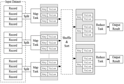
The basic function of the MapReduce model is to iterate over the input, compute key/value pairs from each part of the input, group all intermediate values by key, then iterate over the resulting groups and finally reduce each group. The model efficiently supports parallelism. The programmer can abstract from the issues of distributed and parallel programming, MapReduce implementation deals with issues such as load balancing, network performance, fault tolerance etc. [22]. The Apache Hadoop project [23] is the most popular and widely used open-source implementation of Google’s MapReduce writing in java for reliable, scalable, distributed computing. The MapReduce model is based on two separate steps in an application [34];

- Map: An initial transformation step, in which individual input records are processed in parallel. - Reduce: A summarization step, in which all associated records are processed together by a single entity.

The Hadoop implementation of the MapReduce model is presented inFig. 1shows which split the input into logical

chunks and each chunk is processed independently by a map task. The results of these processing chunks can be physically partitioned into separate sets, which are then sorted. Each sorted chunk is passed to a reduce task.

The Hadoop File System (HDFS) is a file system designed for MapReduce jobs which read input in large chunks, process it, and write chunks of output. For reliability, file data is replicated to multiple storage nodes [34]. HDFS services are provided by two processes:

- NameNode: Manages the file system metadata, and provides management and control services. - DataNode: Provides block storage and retrieval services.

3.2.2. Distributing rationale

SMO takes more than 9 h to train 100

,

000100training examples [28]; training SVM faster with large size training data requires an efficient distributed SMO algorithm. Most of the computation time of the SMO algorithm is spent by updating the optimality condition vectorfiin(2)due to the kernel evaluations which are updated for all points at the iteration [15].

About 90% of the total computation time of SMO is used for updatingfiarray. The solution to this problem is to perform

updatingfiarray in parallel [15]. However this approach incurs large network communication cost due to the large number

of iterations involved. At each step only two points are selected and new step relies on previous data in error cache. The main challenge of distributing SMO is to keep the network communication cost to minimum due to the large number of iterations involved. One possible solution is to partition the training data into smaller parts, train these parts in parallel, and perform a combination of result [28]. We prefer this approach for its simplicity and good result in terms of accuracy.

Another solution is to partition the training data into smaller parts, train these parts in parallel, and perform a combination and a retrain of the combined result [28]. However this approach is time consuming and retraining does not improve the accuracy of the algorithm significantly.

3.2.3. Algorithm design

We have implemented MRSMO using the MapReduce framework. The basic idea of our distributed implementation is similar to Kun et al. [28]. A caching scheme is used to cache the predicted output and update it at each successful step. Kernel cache is used for caching Kernel value between two points which is used during error cache updates.

The algorithm partitions the entire training dataset into smaller subsetsmand allocates each partitioned subset to a

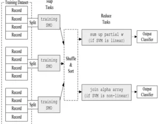
single map task; the number of map tasks is equal to the number of partitions. Each map function optimizes a partition in parallel. In the case of linear SVM the output of each map function is a partial weight vector for the local partition.

⃗

w

Partial

=

l

−

i=1 yiai

⃗

xi (7)

and the value ofbfor that partition. Thereducersums up the partialweight vectorto calculate the globalweight vector.

⃗

w

Global

=

n

−

i=1

⃗

w

Partial

.

(8)

Furthermore, thereducerhas to deal with the value ofbbecause this value is different for each partition; therefore the

reducertask also involves taking the average value ofbfor all partitions. We only need the globalweight vectorand the value

bin order to calculate the SVM output according to the following.

u

= ⃗

w

· ⃗

x

−

b

.

(9)

In the case of nonlinear SVM, the output of each map function is thealpha arrayfor local partition and the value ofb. The

reducersimply joins the partial alpha arrays to produce the globalalpha array. Similar to the linear case thereducerhas to deal with the value ofbbecause this value is different for each partition therefore thereducertakes the average value of b for all partitions. We need thealpha array,band the training data which corresponda

>

0 in order to calculate the SVM output according to the following.

u

=

n

−

i=1 yai i K

(

Xi

,

X

)

+

b

.

(10)

Algorithm 2 shows the pseudocode MRSMO; in line 1 p indicates the total number of training data partitions.

{

lm

}

p m=1



k=1→plm

=

lis a subset of all the training data patterns allocated to partitionm. Lines 1–12 are used to show the optimization process of SMO for each partition; in each line only two points are used to jointly optimize at each iteration.

The process continues until the optimality gap conditionbm

low

≤

bmup

+

2

τ

is satisfied. Lines 13–19 are used to show the assembling results from each partition to create global result; that is globalweight vectorif SVM is linear, globalalpha array, and the value of b if SVM in non-linear.

Algorithm 2: MRSMO Algorithm

Input: training dataxm

i , labelsymi ,

Output: sum of weight vector,

α

array,band SVs 1: p

=

number of partition

{

lm

}

p_m=1

,



m=1→pl m

=

_l 2: Initialize:

α

_im

=

0

,

f_im

= −

ym_i 3: Compute:bm high,Ihighm ,bmlow

,

Ilomw 4: Update

α

_Ihighm and

α

m_Ilow 5: repeat

6: Updatef_im

7: Compute:bm_high,I_highm ,bm_low,I_lom_w

8: Update

α

_Ihighm and

α

m_Ilow 9: untilbm

low

≤

bmup

+

2

τ

10: Update the thresholdbm

11: Store the new

α

m1 and

α

m2 values 12: Update vector

w

mif SVM is linear 13: Calculate the value b;b

=

∑

p

i=1bm

/

p 14: If (SVM is linear) 15: Calculate W;

w

=

∑

p i=1

w

m 16: Else 17: ObtainSV_setm_;s

v

m

= {

α

im

>

0

}

18: Create SV set;



_m=1→ps

v

m 19: Store allxiwhere

α

i

>

o

Fig. 2. The MRSMO architecture.

Fig. 3. Image annotation system architecture. We summarize the structure of the MRSMO as follows:

- Divide the training set intomrandom subsets of fixed size. - Allocate each partition to a single map task.

- Each map function trains the partition; the output of each map function is a partialweight vectorand the value ofbif SVM is linear. In the case of nonlinear SVM, the output of each map function is thealpha arrayand the value ofb.

- Thereducertakes the average ofbvalues, sums up the partialweight vectorsto produce globalweight vectorif SVM is

linear. The reducer simply joins the partialalpha arraysto produce the globalalpha arrayif SVM is nonlinear.

MRSMO Architecture is presented inFig. 2.

4. Experimental results

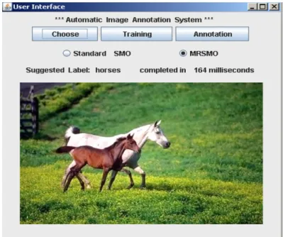
In order to evaluate the efficiency of the MRSMO, we have implemented a prototype image annotation system using Java programming language and the WEKA package [36]. The image annotation systems classify visual features into pre-defined classes.Fig. 3shows the architecture of the system; first images are segmented into blocks. Then, the low-level features are extracted from the segmented images. Each segmented block is represented by feature vectors. Next stage is to assign the low-level feature vectors to pre-defined categories. The system learns the correspondence between low level visual features and image labels. Combination of low-level MPEG-7 descriptors such as scalable color [37] and edge histogram [37] is used. In training stage, the classifier is fed with a set of training images in the form of attribute vectors with the associated labels. After a model is trained, it is able to classify an unknown instance, into one of the learned class labels in the training set.

User interface of the prototype system which supports automatic annotation of images using standalone and MRSMO classifiers is presented inFig. 4.

Fig. 4. A snapshot of the image annotation system.

4.1. Image corpora

The images are collected from the Corel database [38]. Images are classified into 10 classes, and each class of images has one label associated with it. The 10 pre-defined labels are people, beach, mountains, bus, food, dinosaur, elephant, horses, flowers and historic. Typical image sizes of 384

×

256 pixels are used in the training process. Low level features of the images are extracted using the LIRE (Lucene Image REtrieval) library [39]. After extracting low level features, a typical image takes the following basic form;

0

,

256

,

12

,

1

,

−

56

,

3

,

10

,

1

,

18

, . . . ,

2

,

0

,

0

,

1

,

0

,

0

,

0

,

0

,

0

,

0

,

0

,

0

,

0

,

beach

.

Each image is represented by 483 attributes, the last attribute indicates class name which indicates the category to which the image is belonged.

4.2. Performance evaluation

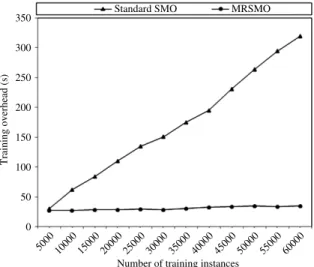
A number of tests was carried out on 3 Dell computers, Linux Fedora 11, RAM- 3.00 GB, Processor 2.4 GHz. The experiment shows that the efficiency of the MRSMO increases with the increase of the number of processors, the speed of training SVM

using 12mappersis around 11 times higher than the standalone SMO. The MRSMO is extremely useful for large size training

data. Standard SMO and MRSMO were evaluated from the aspects of accuracy in annotating images and efficiency in training

the models. The comparison of training times of standard SMO and MRSMO in binary classification is shown inFig. 5.

Furthermore, we compared the accuracy level of the standard SMO and MRSMO algorithms in classification and presented the results inFig. 6. In total 50 unlabeled images were tested (10 images at a time), the average accuracy level was considered. It is clear that the parallelization of SMO has not affected the accuracy level significantly. Results show that the MRSMO achieves 93% accuracy level compared to 94% in the standard SMO. The differences between the generalization performances achieved by standard SMO and MRSMO are very small and could be neglected in many cases. Although a very large number of partitions could affect the level of accuracy of MRSMO, however if the input data is partitioned randomly and the size of partitions are large enough, the effect on accuracy can be quite small [28].

4.2.1. Multiclass classification (one against all)

Multi-class classification on MRSMO was performed by one against all technique [40], that is at each map step only one class of training instances is optimized against the rest of the classes. We consider ann-class problem. We need to determine

ndirect decision functions that separate one class from the rest of the classes. LetDibe theith decision function with the

maximum margin that separates classifrom the rest of the classes:

Di

(

x

)

=

w

ig

(

x

)

+

bi (11)

where

w

iis thel-dimensional vector, g(x) is the mapping function that mapsxonto thel-dimensional feature space, andbi is the bias. The hyperplaneDi

(

x

)

=

0 creates the separating hyperplane, training data belonging to classisatisfyDi

(

x

)

≥

1

Standard SMO 350 300 250 200 150 Training overhead (s)

Number of training instances 100 50 0 5000 10000 15000 20000 25000 30000 35000 40000 45000 5000 0 55000 60000 MRSMO

Fig. 5. Comparison of training times of standard SMO and MRSMO in binary classification.

Standard SMO 1 0.9 0.8 0.7 0.6 Level of accuracy

Number of training instances (1000) 0.4 0.5 0.2 0.3 0 0.1 0.5 1 1.5 2 2.5 3 3.5 4 4.5 5 MRSMO

Fig. 6. Comparison of accuracy level of SMO and MRSMO in multiclass classification.

and training data belonging to the rest of the classes satisfyDi

(

x

)

≤

1. In classification, if for the input vectorx,Di

(

x

) >

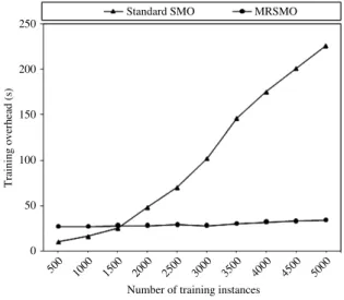
0 is satisfied for onei,xis classified into classi. This is because only the sign of the decision function is used.

A total of 5000 images are used in training process, images are classified into 10 classes, and each class of images has one label associated with it. The 10 pre-defined labels are people, beach, mountains, bus, food, dinosaur, elephant, horses, flowers and historic. MRSMO displays a high level of efficiency in training process compared to the standard SMO as shown

inFig. 7.

5. Conclusion and future work

In this paper, we have presented and evaluated a MapReduce based distributed SVM algorithm that capitalizes on the scalability, parallelism and resiliency of the MapReduce framework for automatic image annotation. The performance of the MRSMO algorithm is evaluated in an experimental environment. By partitioning the training dataset into smaller subsets and optimizing the partitioned subsets across a cluster of multiple computing nodes, the MRSMO algorithm reduces the training time significantly while maintaining a high level of accuracy in binary and multiclass classifications especially for large size training dataset.

As part of future research work, we are planning to introduce load balancing techniques in order to achieve optimal resource utilization. We believe that load balancing would further enhance the performance of our algorithm in terms of speed. In this version, multiclass classification is performed using one against all technique. We are planning to implement a MapReduce based distributed multiclass SMO using one against one technique which is considered to be more efficient, For

Standard SMO 250

200

150

Training overhead (s)

Number of training instances 100

50

0

500 _{1000 1500 2000 2500 3000 3500 4000 4500 5000}

MRSMO

Fig. 7. Comparison of training times of SMO and MRSMO in multiclass classification.

n class problem, the classifier generatesn

(

n

−

1

)/

2 submodels, wherenis the number of classes. Each model solves a binary subproblem, which is the most computationally expensive part in training multiclass SVM. We are planning to consider heterogeneity in training datasets as well as available processors in a cluster environment, in which the computation tasks have to be distributed and scheduled among all of the available processors equally to improve the overall performance.

References

[1] A. Smeulders, M. Worring, S. Santini, A. Gupta, R. Jain, Content based image retrieval at the end of the early years, IEEE Trans. Pattern Anal. Mach. Intell. 22 (12) (2000) 1349–1380.

[2] C. Tsai, C. Hung, Automatically annotating images with keywords: a review of image annotation, Recent Patents on Comput. Sci. 1 (2008) 55–68. [3] W-T. Wong, S-H. Hsu, Application of SVM and ANN for image retrieval, European J. Oper. Res. 173 (2006) 938–950.

[4] Y. Gao, J. Fan, Semantic image classification with hierarchical feature subset selection, in: Proceedings of the ACM Multimedia Workshop on Multimedia Information Retrieval, Hilton, Singapore, Nov. 10–11, 2005, pp. 135–142.

[5] M. Boutell, J. Luo, X. Shen, C.M. Brown, Learning multi-label scene classification, Pattern Recognit. 37 (5) (2004) 1757–1771. [6] Y. Chen, J.Z. Wang, Image categorization by learning and reasoning with regions, J. Mach. Learn. Res. 5 (2004) 913–939. Y.

[7] C. Cusano, G. Ciocca, R. Schettini, Image annotation using SVM, in: Proceedings of SPIE Conference on Internet Imaging V, San Jose, California, 5304, Jan. 19–20 2004, pp. 330–338.

[8] J. Fan, Y. Gao, H. Luo, G. Xu, Automatic image annotation by using concept-sensitive salient objects for image content representation, in: Proceedings of the 27th Annual International ACM SIGIR Conference on Research and Development in Information Retrieval, Sheffield, UK, July 25–29 2004, pp. 361–368.

[9] B. Le Saux, G. Amato, Image recognition for digital libraries, in: Proceedings of the ACM Multimedia Workshop on Multimedia Information Retrieval, New York, Oct. 15-16, 2004.

[10] N. Cristianini, J. Shawe-Taylor, An Introduction to Support Vector Machines and Other Kernel-Based Learning Methods, Cambridge University Press, 2000, pp. 1–172.

[11] C. Waring, Xiuwen Liu, Face detection using spectral histograms and SVMs, IEEE Trans. Syst. Man Cybern. Part B: Cybernetics 35 (2005) 467–476. [12] F. Colas, P. Brazdil, Comparison of SVM and some older classification algorithms in text classification tasks, in: IFIP-AI 2006, World Computer Congress,

Santiago de Chile, Chile, Springer, vol. 217, 1861–2288, 2006, pp. 169–178.

[13] T. Do, V. Nguyen, F. Poulet, Speed up SVM algorithm for massive classification tasks, in: ADMA’08: Proceedings of the 4th International Conference on Advanced Data Mining and Applications, Berlin, Heidelberg, Springer-Verlag, vol. 5139, 1611–3349, 2008, pp. 147–157.

[14] N. Khalid Alham, M. Li, S. Hammoud, H. Qi, Evaluating machine learning techniques for automatic image annotations, in: Proc. of FSKD09, IEEE CS, Aug.2009.

[15] L. Cao, S. Keerthi, Chong-Jin Ong, J. Zhang, U. Periyathamby, Xiu Ju Fu, H. Lee, Parallel sequential minimal optimization for the training of support vector machines, IEEE Trans. Neural Netw. 17 (2006) 1039–1049.

[16] R. Collobert, S. Bengio, Y. Bengio, A Parallel Mixture of SVMs for Very Large Scale Problems, 2002.

[17] Guang-Bin Huang, K. Mao, Chee-Kheong Siew, De-Shuang Huang, Fast modular network implementation for support vector machines, IEEE Trans. Neural Netw. 16 (2005) 1651–1663.

[18] T. Hazan, A. Man, A. Shashua, A parallel decomposition solver for SVM: distributed dual ascend using Fenchel duality, in: Computer Vision and Pattern Recognition, 2008. CVPR 2008. IEEE Conference, 2008, pp.1–8.

[19] Yumao Lu, V. Roychowdhury, L. Vandenberghe, Distributed parallel support vector machines in strongly connected networks, IEEE Trans. Neural Netw. 19 (2008) 1167–1178.

[20] J. Dong, A. Krzyżak, C. Suen, A fast parallel optimization for training support vector machine, Mach. Learn. Data Mining Pattern Recognit. (2003) 96–105.

[21] B. Catanzaro, N. Sundaram, K. Keutzer, Fast support vector machine training and classification on graphics processors, in: Proceedings of the 25th International Conference on Machine Learning, ACM, Helsinki, Finland, 2008, pp. 104–111.

[22] R. Lämmel, Google’s mapreduce programming model — revisited, Sci. Comput. Program. 70 (Jan.2008) 1–30. [23] Apache Hadoop, Available:http://hadoop.apache.org/.

[24] G. Zanghirati, L. Zanni, A parallel solver for large quadratic programs in training support vector machines, Parallel Comput. 29 (2003) 535–551. [25] S. Winters-Hilt, K. Armond, Distributed SVM learning and support vector reduction submitted to BMC bioinformatics, 2008, available:http://cs.uno.

edu/∼_{winters/SVM_SWH_preprint.pdf.}

[26] D. Bickson, E. Yom-Tov, D. Dolev, A Gaussian belief propagation solver for large scale support vector machines. 2008, available:http://www.cs.huji. ac.il/∼_{dolev/pubs/dd-ECCS08.pdf.}

[27] H. Graf, E. Cosatto, L. Bottou, I. Durdanovic, V. Vapnik, Parallel support vector machines: the cascade SVM, Neural Information Processing Systems (2004).

[28] D. Kun, L. Yih, A. Perera, Parallel SMO for training support vector machines, SMA 5505 Project Final Report. May 2003, available atwww.geocities.com/ asankha/Contents/Education/APC-SVM.pdf.

[29] B.C. Kuszmaul, Cilk provides the ‘‘best overall productivity’’ for high performance computing: (and won the HPC challenge award to prove it), in: Proceedings of the Nineteenth Annual ACM Symposium on Parallel Algorithms and Architectures, ACM, San Diego, California, USA, 2007, pp. 299–300.

[30] D. Gillick, A. Faria, J. DeNero, Mapreduce: distributed computing for machine learning, 2006, [Online] available:www.icsi.berkeley.edu/~arlo/ publications/gillick_cs262a_proj.pdf.

[31] C. Chu, S. Kim, Y. Lin, Y. Yu, G. Bradski, A. Ng, K. Olukotun, Map-reduce for machine learning on multicore, in: NIPS, MIT Press, 2006, pp. 288, 281. [32] J.C. Platt, Sequential minimal optimization:a fast algorithm for training support vector machines. 1998, available:http://research.microsoft.com/enus/

um/people/jplatt/smoTR.pdf.

[33] S.S. Keerthi, S.K. Shevade, C. Bhattacharyya, K.R.K. Murthy, Improvements to platt’s SMO algorithm for svm classifier design, Neural Computing 13 (2001) 637–649.

[34] J. Venner, Pro Hadoop, Springer, 2009, pp. 1–407.

[35] S. Ghemawat, H. Gobioff, S. Leung, The google file system, SIGOPS Oper. Syst. Rev. 37 (2003) 29–43.

[36] Weka, 3 — Data mining with open source machine learning software in Java, available at:http://www.cs.waikato.ac.nz/ml/weka/.

[37] T. Sikora, The MPEG-7 visual standard for content description-an overview: 696-702. 2001, available:http://www.ee.columbia.edu/∼_{sfchang/course/} vis/REF/sikora01.pdf.

[38] Corel image databases, available:www.corel.com.

[39] Lire, An open source java content based image retrieval library available at:http://www.semanticmetadata.net/lire/.