Approximation Algorithms for Distributionally Robust Stochastic Optimization

(1)

Approximation Algorithms for

Distributionally Robust

Stochastic Optimization

by

André Linhares Rodrigues

A thesis

presented to the University of Waterloo in fulfillment of the

thesis requirement for the degree of Doctor of Philosophy

in

Combinatorics and Optimization

Waterloo, Ontario, Canada, 2019

(2)

Examining Committee Membership

The following served on the Examining Committee for this thesis. The decision of the Examining Committee is by majority vote.

External Examiner: Nicole Megow

Professor, Institute of Computer Science, Universität Bremen

Supervisor: Chaitanya Swamy

Professor, Department of Combinatorics and Optimization, University of Waterloo

Internal Member: Jochen Könemann

Professor, Department of Combinatorics and Optimization, University of Waterloo

Internal Member: Laura Sanità

Associate Professor, Department of Combinatorics and Optimization, University of Waterloo

Internal-External Member: Lap Chi Lau

Associate Professor, Cheriton School of Computer Science, University of Waterloo

(3)

Author’s Declaration

This thesis consists of material all of which I authored or co-authored: see Statement of Contributions included in the thesis. This is a true copy of the thesis, including any required final revisions, as accepted by my examiners.

(4)

Statement of Contributions

The results in this thesis are chiefly based on the publication [85], which is joint work with my supervisor Chaitanya Swamy. I have made a major contribution toward this publication.

(5)

Abstract

Two-stage stochastic optimization is a widely used framework for modeling uncertainty, where we have a probability distribution over possible realizations of the data, called sce-narios, and decisions are taken in two stages: we take first-stage actions knowing only the underlying distribution and before a scenario is realized, and may take additional second-stage recourse actions after a scenario is realized. The goal is typically to minimize the total expected cost. A common criticism levied at this model is that the underlying probability distribution is itself often imprecise. To address this, an approach that is quite versatile and has gained popularity in the stochastic-optimization literature is the two-stage distri-butionally robust stochastic model: given a collection D of probability distributions, our

goal now is to minimize the maximum expected total cost with respect to a distribution inD.

There has been almost no prior work however on developing approximation algorithms for distributionally robust problems where the underlying scenario collection is discrete, as is the case with discrete-optimization problems. We provide frameworks for designing approximation algorithms in such settings when the collectionDis a ball around a central

distribution, defined relative to two notions of distance between probability distributions: Wasserstein metrics (which include the L1 metric) and the L∞ metric. Our frameworks

yield efficient algorithms even in settings with an exponential number of scenarios, where the central distribution may only be accessed via a sampling oracle.

For distributionally robust optimization under a Wasserstein ball, we first show that one can utilize the sample average approximation (SAA) method—solve the distribution-ally robust problem with an empirical estimate of the central distribution—to reduce the problem to the case where the central distribution has a polynomial-size support, and is represented explicitly. This follows because we argue that a distributionally robust problem can be reduced in a novel way to a standard two-stage stochastic problem with bounded inflation factor, which enables one to use the SAA machinery developed for two-stage stochastic problems. Complementing this, we show how to approximately solve a frac-tional relaxation of the SAA problem (i.e., the distribufrac-tionally robust problem obtained by replacing the original central distribution with its empirical estimate). Unlike in two-stage {stochastic, robust} optimization with polynomially many scenarios, this turns out to be quite challenging. We utilize a variant of the ellipsoid method for convex optimization in conjunction with several new ideas to show that the SAA problem can be approximately solved provided that we have an (approximation) algorithm for a certain max-min prob-lem that is akin to, and generalizes, thek-max-min problem—find the worst-case scenario consisting of at most k elements—encountered in two-stage robust optimization. We

(6)

ob-tain such an algorithm for various discrete-optimization problems; by complementing this via rounding algorithms that provide local (i.e., per-scenario) approximation guarantees, we obtain the first approximation algorithms for the distributionally robust versions of a variety of discrete-optimization problems including set cover, vertex cover, edge cover, facility location, and Steiner tree, with guarantees that are, except for set cover, within O(1)-factors of the guarantees known for the deterministic version of the problem.

For distributionally robust optimization under an L∞ ball, we consider a fractional

relaxation of the problem, and replace its objective function with a proxy function that is pointwise close to the true objective function (within a factor of2). We then show that we can efficiently compute approximate subgradients of the proxy function (for a certain notion of approximate subgradients introduced by Shmoys and Swamy [114]), provided that we have an algorithm for the problem of computing thet worst scenarios under a given

first-stage decision, given an integert. We can then approximately minimize the proxy function

via a variant of the ellipsoid method by [114], and thus obtain an approximate solution for the fractional relaxation of the distributionally robust problem. Complementing this via rounding algorithms with local guarantees, we obtain approximation algorithms for distributionally robust versions of various covering problems, including set cover, vertex cover, edge cover, and facility location, with guarantees that are withinO(1)-factors of the guarantees known for their deterministic versions.

(7)

Acknowledgements

First, I would like to thank Chaitanya Swamy for being such a dedicated supervisor. Our weekly meetings have been a constant source of inspiration and encouragement, and have been invaluable for the completion of this thesis. I am also thankful for his very detailed and constructive advice and feedback regarding academic writing and talks, as well as other academic and career matters.

I would also like to thank the other members of the examining committee, namely Nicole Megow, Jochen Könemann, Laura Sanità, and Lap Chi Lau, for devoting time to reading this thesis and providing helpful feedback.

Thank you to the other C&O professors from whose courses I have benefited, and with whom I had the pleasure to collaborate, especially Ricardo Fukasawa, Jochen Könemann, Joseph Cheriyan, and Laura Sanità. I am also grateful to the members of the department’s administrative team for their assistance, particularly Melissa, Carol, and Megan; and to my fellow graduate students for their friendship.

Finally, I am deeply grateful to my parents for their unwavering and unconditional support.

(8)

List of Figures

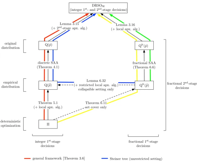
6.1 Problem reductions utilized by our frameworks for DRS optimization under a Wasserstein ball. . . 88

(12)

List of Tables

3.1 Approximation factors for DRS optimization under a Wasserstein ball. . . 29 3.2 Approximation factors for DRS optimization under an L∞ ball. . . 33 6.1 Approximation factors for DRS optimization under a Wasserstein ball. . . 87 7.1 Approximation factors for DRS optimization under an L∞ ball. . . 136

(13)

Chapter 1

Introduction

In this chapter, we introduce the model studied in this thesis in Section 1.1, and give a high-level overview of our main contributions in Section 1.2 (we postpone a more detailed overview to Section 3.3). In Section 1.3, we list some basic mathematical definitions, notation, and conventions that we use throughout this thesis. In Section 1.4, we outline the contents of each of the following chapters.

1.1

The distributionally robust stochastic optimization

framework

In practical applications of optimization, one often encounters problems involving uncertain parameters—for example, parameters that cannot be measured exactly, or that depend on future events that cannot be predicted with certainty. A naive approach for tackling such problems consists in computing estimates of all the uncertain parameters, and solving the deterministic problem obtained by utilizing these estimates in lieu of the real (uncertain) parameters. Unsurprisingly, this approach can lead to unsatisfactory (i.e., low-quality or even infeasible) decisions. Therefore, developing models that incorporate uncertainty in the parameters is crucial for making satisfactory decisions in such settings.

An important and widely used model is thetwo-stage recourse model, wherein we seek to take actions in two stages. In the first stage, we make ahere-and-now decisionx, using only

limited information (or no information at all) on the uncertain parameters. In the second stage, ascenarioAis revealed (i.e., the values of the uncertain parameters become known),

(14)

scenario. The second-stage actions are typically costlier than the corresponding first-stage actions, as they may entail making decisions in rapid reaction to the observed scenario (e.g., deploying resources with smaller lead time).

An oft-cited prototypical example is two-stage facility location, wherein we need to decide where to set up facilities to serve clients, in the face of uncertain client demands. We can open some facilities initially, given only limited information about demands; after a specific demand pattern is realized, we can take additional recourse actions such as opening more facilities, incurring their recourse costs. Different objective functions can be adopted, depending in particular on the level of risk aversion of the decision maker and on the granularity of the information on the uncertain parameters that is made available to them. This choice leads to several variants of the two-stage recourse model; two popular models are two-stage {robust, stochastic} optimization. We briefly define these models and discuss some issues that may arise when utilizing them. We then define the model that is the focus of this thesis, namely two-stage distributionally robust stochastic optimization, which mitigates these issues by interpolating between robust and stochastic optimization. We defer a discussion of previous work related to these models to Chapter 2.

Two-stage robust optimization. If no information on the likelihood of the different scenarios is available, or if the decision maker is highly averse to risk, a suitable model is two-stage robust optimization, wherein we seek to minimize the total cost in the worst-case scenario. Formally, we consider the problem

min (x,{zA_} A∈A) (cost of x) + max A∈A cost of zA ,

where A denotes the set of all possible scenarios. While this model can be appealing in

the circumstances mentioned above, it is in some cases overly cautious, leading to severely undesirable decisions. One potential issue is that the existence of a single catastrophic scenario may force us to take first-stage actions that are unhelpful for all the remaining scenarios, and this may occur even if such a scenario is extremely unlikely.

Two-stage stochastic optimization. If some information on the likelihood of the dif-ferent scenarios is available, a less conservative approach is to leverage this information and seek instead a decision that is desirablein expectation. This gives rise to another prominent model, namely two-stage stochastic optimization, wherein we seek to minimize the total expected cost incurred (with respect to the scenario realized). That is, if the scenario is

(15)

modeled as a random variable drawn fromAaccording to a probability distributionp, then

we consider the problem min (x,{zA_} A∈A) (cost of x) +_EA∼p cost of zA ,

whereEA∼p[·]denotes the expectation whenA is chosen according top. A significant issue

that occurs when using this model to capture real-world applications, which is a common source of criticism, is that the probability distributionp modeling the uncertainty is itself

often imprecise. Usually, one computes a distribution p based on some historical data.

While historical data may serve as a reasonably accurate representation of the behavior of the underlying unknown parameters, it is not sufficient to give an exact characterization of this behavior. For example, a scenario that occurs with extremely low (but positive) probability is unlikely to be observed in the historical data, so an empirical distribution computed in this way would be likely to incorrectly assign probability zero to such a scenario. As another example, suppose we observe a sequence ofN2 _{coin tosses, such that}

in each batch of N coin tosses the number of heads is between 0.49N and 0.51N. Then,

while it is possible that this sequence arose from a coin without bias (i.e., the probability of heads is equal to0.5), all we can really say is that there is a range of biases concentrated around0.5under which the above statistic is likely.1

Two-stage distributionally robust stochastic optimization. The issues encoun-tered in {robust, stochastic} optimization that we discussed above motivate the study of models that leverage information on the likelihood of the different scenarios, but do not assume knowledge of the exact underlying distribution. As mentioned before, one usually models the distribution to be statistically consistent with some historical data, so we re-ally have a collection of probability distributions, and a more robust approach is to hedge against the worst-possible probability distribution in this collection. (Note that the worst-possible distribution depends on the chosen first-stage decision x.) This gives rise to the

model that is the focus of this thesis, namely two-stage distributionally robust stochastic optimization. The setup is similar to that of the two-stage stochastic model, but we now have a collectionDof probability distributions, which we refer to as theambiguity set; our goal is to minimize the maximum expected total cost with respect to a distribution inD.

1_{More precisely, for any confidence level}_{δ >}_{0, there is some}_{ε >}₀ _{(depending on}_δ_and_{N) such that}

for any coin with biasp ∈[0.5−ε,0.5 +ε], the probability of seeing the above statistics from a coin of

(16)

That is, we consider the problem min (x,{zA_} A∈A) (cost of x) + sup p∈DEA ∼p cost of zA .

Distributionally robust stochastic (DRS) optimization is a versatile approach dating back to Scarf [103] that has regained interest recently in the Operations-Research litera-ture, where it is sometimes calleddata-driven or ambiguous stochastic optimization (see, e.g., [16, 43, 52,126], and the references therein).

The two-stage DRS model also serves to nicely interpolate between the extremes of: (a) two-stage stochastic optimization, which optimistically assumes that the underlying distributionpis known precisely (which can be captured by settingD={p}); and (b)

two-stage robust optimization, which abandons the distributional view and seeks to minimize the maximum cost incurred in a scenario, thereby adopting the overly cautious approach of being robust againstevery possible scenario, regardless of how likely it is for a scenario to materialize (this can be captured by letting D = {all distributions overA}, where A

is the scenario collection in the two-stage robust problem; alternatively, we could take D

to be the collection of all distributions over A concentrated at a single scenario A ∈ A).

Both extremes can lead to suboptimal decisions: with robust optimization, the presence of a single scenario, however unlikely, may lead to decisions that are undesirable for all other scenarios; with stochastic optimization, the optimal solution for a specific distribution p

could be quite suboptimal even for a “nearby” distributionq, as illustrated by the following

example.

Example: consider an instance oftwo-stage set cover with a single elementeand a single

setS ={e}. Suppose that the first-stage and second-stage costs of buying S are 1 and M_ε respectively, where ε ∈ (0,1] and M 1. The collection of scenarios is A := {∅,{e}}; a

scenario specifies which elements must be covered. Let p be the probability distribution

with p∅ = 1 and p{e} = 0, and q be the probability distribution with q∅ = 1− ε and

q{e} = ε. The optimal solution under p is to not buy S in the first stage; this incurs cost

(1−ε)·0 +ε· M

ε =M under q, but the optimal solution under q is to buy S in the first

stage and incur cost 1. This shows that even if kp−qk ≤ O(ε), we can find instances where an optimal decision forp is undesirable under q.

(17)

1.2

Our contributions

Despite the modeling benefits and popularity of DRS optimization, to our knowledge, there has been almost no prior work on developing approximation algorithms for discrete two-stage DRS problems, and, more generally, for two-stage DRS problems with adiscrete underlying scenario set (as is the case in discrete optimization). (The exception is Agrawal, Ding, Saberi, and Ye [2], which we discuss in Section 2.3; peripherally related is Wu, Du, and Xu [130], who consider a DRS version of facility location where the uncertainty only affects the costs and not the constraints, which yields a much simpler and more restric-tive model.) In this thesis, we provide frameworks for designing efficient approximation algorithms in such settings. In this section, we give a high-level overview of our contri-butions. We refer the reader to Section 3.3 for a more precise and detailed exposition of our main results and the techniques we use to obtain them, as well as a summary of the approximation factors we obtain for various applications.

We develop general frameworks for designing approximation algorithms for discrete two-stage DRS optimization problems where the ambiguity setDis a ball around a central

distribution ˚p under some metric L over probability distributions; that is, we have D =

{p:L(˚p, p)≤r}, where r > 0 is the radius of the ball. We consider three choices for the metric L: (i) the L∞ metric, defined by L∞(p, q) := maxA∈A|pA−qA|; (ii) the 1₂L1 metric

(also known as thetotal-variation distance), defined by 1₂L1(p, q) := 1₂

P

A∈A|pA−qA|; and

(iii) Wasserstein metrics, a rich class of metrics obtained by lifting an underlying scenario metric` :A × A →_R+ to a metric over distributions, which includes the 1₂L1 metric as a

special case (see Definition 3.1). Our results hold under thebounded-inflation assumption, which roughly speaking encodes that each first-stage action has a corresponding second-stage action whose cost is at most λ times higher, for a given inflation factor λ≥ 1. The cardinality of the scenario collection A may be very large, even exponential in the input size; the central distribution˚p may only be accessed via a sampling oracle.

DRS optimization under a Wasserstein ball. For a first-stage decision x and a

scenario A, let g(x, A) denote the minimum cost incurred in extending x to a feasible

solution for A, if we allowfractional second-stage decisions. For a broad class of problems, we relate the approximability of a discrete two-stage DRS optimization problem under a Wasserstein ball (where the Wasserstein metric is defined relative to a scenario metric

` :A × A →_R+) to the approximability of the problem of computing

g(x, y, A) := max

A0_∈A{g(x, A

0

(18)

given an integer first-stage decisionx, a number y ≥0, and a scenario A. Informally, our

main result (see Theorem3.6) is that we can compute anO(αβ1β2ρ)-approximate solution

for a discrete DRS problem in poly(input size, λ) time as long as we have the following three ingredients:

(i) a second-stage (LP-relative) α-approximation algorithm, which is an algorithm that given an integer first-stage decision xand a scenarioA, computes an integer

second-stage decisionzAof cost at mostα·g(x, A)such that x, zAis feasible for scenario A;

(ii) a (β1, β2)-approximation algorithm for computing g(x, y, A), which is an algorithm

that given a tuple (x, y, A)computes a scenario A ∈ A such that

g x, A−y·` A, A≥max A0_∈A 1 β1 g(x, A0)−β2y·`(A, A0) ; and

(iii) a local ρ-approximation algorithm, which is an algorithm that rounds a fractional first-stage decision to an integer one while incurring at most a ρ-factor blow-up in

the first-stage cost, and in the cost of each scenario.

The proof of the result above has two main components, which are of independent interest. The first component (see Chapter 4) is a sample-average-approximation (SAA) result for DRS optimization under a Wasserstein ball, which reduces the discrete DRS problem (with a central distribution˚p given by a sampling oracle) to a collection of SAA

problems with fractional second-stage decisions, wherein ˚p is replaced with an empirical

estimate bp, constructed using poly(input size, λ) samples. The second component (see Chapter 5) is an approximation algorithm for the SAA problems; this is obtained via a variant of the ellipsoid method, using ingredients (ii) and (iii). Combining these two components, we obtain an integer first-stage decision, and fractional second-stage decisions, which we then convert into integer second-stage decisions using ingredient(i).

DRS optimization under anL∞ ball. Our main result for discrete DRS optimization

under anL∞ ball (see Theorem3.9) is that, for a broad class of problems, we can compute

anO(ρ)-approximate solution in poly input size, λ,1_r time, as long we have the following

ingredients:

(i) an algorithm that given a fractional first-stage decision and a numbert≤min|A|,1

r ,

computes thetworst scenarios under the given first-stage decision inpoly(input size, t) time; and

(19)

(ii) a local ρ-approximation algorithm.

The proof of this result is presented in Chapter 7, and relies on a variant of the ellipsoid method based on approximate subgradients by Shmoys and Swamy [114].

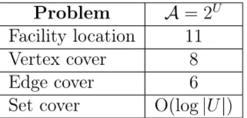
Applications. By applying the frameworks mentioned above for DRS optimization un-der a Wasserstein ball or an L∞ ball, and furnishing the ingredients required by them, we

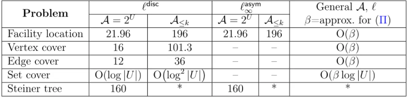
obtain the first approximation results for DRS versions of a variety of problems, including set cover, edge cover, vertex cover, facility location, and Steiner tree. Tables 3.1 and 3.2 show the approximation factors that we obtain for various choices of the scenario collection

A and of the scenario metric` (in the Wasserstein setting).

1.3

Basic definitions, notation, and conventions

In this section we state some basic definitions, notation, and conventions that will be used throughout the thesis.

We use a := b to denote the fact that a is defined as b. For a set S, we denote by

2S the collection of all subsets of S. For a vector u ∈ _RS_{, indexed by} _S_{, we denote by}

kuk:=pP_e_∈_Su2

e its Euclidean norm, and by supp(u) :={e ∈S :ue 6= 0}its support. For

an integern, we let [n] :={1,2, . . . , n} if n ≥1, and [n] :=∅ otherwise.

We denote by log_ba the logarithm of ato base b. We often only care about the

asymp-totic growth of an expression; in such cases, the base is not relevant and we may omit it. We denote by lna the natural logarithm of a.

We denote byPr[E]the probability of an eventE. We denote by_Eξ∼p[v]the expectation

of an expressionv when a random variable ξis randomly chosen according to a probability

distribution p. When the distribution of the random variable ξ is clear from the context,

we may simply writeE[v].

Consider a real-valued function f : D → _R, where D ⊆ _Rn_{. A vector} _d _∈

Rn is a

subgradient of f at u ∈ D if we have f(v) ≥ f(u) +d|(v −u) for every v ∈ D. It is

well known that a convex function has a subgradient at every point in the relative interior of its domain (see, e.g., Theorem 23.4 of Rockafellar [99]). We say that f is K-Lipschitz continuous (for some nonnegative number K) if we have |f(u)−f(v)| ≤ Kku−vk for

everyu, v ∈D. The smallest numberK (if any) for which this holds is called the Lipschitz constant of f. The following well known result shows that the existence of subgradients

(20)

with bounded Euclidean norm implies a bound on the Lipschitz constant of f (see, e.g.,

Claim 4.11 of Shmoys and Swamy [114]).

Lemma 1.1. Let f :D→_R be a convex function, where D⊆_Rn_{. Suppose that for every}

point u∈D there exists a subgradient of f at u with Euclidean norm at most K. Then f

isK-Lipschitz continuous.

For parameters(n1, . . . , nk), we say that an expressionf(n1, . . . , nk)is poly(n1, . . . , nk)

if there exist (absolute) constants c1, c2 > 0 such that f(n1, . . . , nk) ≤ (n1n2. . . nk)c1

for every n1, . . . , nk ≥ c2. We also write f(n1, . . . , nk) = poly(n1, . . . , nk) with the same

meaning.

This thesis deals mostly withNP-hard problems, so we focus on designingapproximation algorithms. For an instance I of an optimization problem P, we denote by OPT(I) its optimal value (if it exists). An α-approximate solution for I (where α ≥ 1) is a feasible solution that attains objective value:

• at most α·OPT(I), if P is a minimization problem; and • at least _α1 ·OPT(I), if P is a maximization problem.

Anα-approximation algorithmfor P is an algorithm that, given any instance of P, computes in polynomial time an α-approximate solution for it. We also use the following broader

terminology to allow additive approximation, and algorithms whose running time depends on additional parameters other than the input size. Anapproximate solutionfor an instance

I is a feasible solution whose objective value is within some bounded multiplicative factor

and/or additive term of OPT(I). Anapproximation algorithm for P is an algorithm that, given any instanceI of P, computes an approximate solution for I.

1.4

Organization of the thesis

In Chapter 2, we give an overview of relevant previous work on robust, stochastic, and distributionally robust stochastic optimization. In Chapter3, we formally define the DRS optimization model that we study and the class of problems to which our frameworks apply. We then give a summary of the main results we obtain for DRS optimization under a Wasserstein ball or an L∞ ball (see Section 3.3), and prove some preliminary results.

The next two chapters contain the two components of our framework for DRS optimization under a Wasserstein ball: Chapter4presents an SAA result, reducing the original problem

(21)

(with a central distribution given by a sampling oracle) to a collection of SAA problems with an explicit central distribution; Chapter5shows how to approximately solve the SAA problems. In Chapter6, we show how to combine the two components to obtain our main result for DRS optimization under a Wasserstein ball (Theorem 3.6). We then apply our framework to obtain approximation algorithms for DRS versions of various problems under a Wasserstein ball, namely set cover, edge cover, vertex cover, facility location, and Steiner tree. In Chapter 7, we present our framework for DRS optimization under an L∞ ball,

and prove our main result in this setting (Theorem 3.9). We then apply our framework to obtain approximation algorithms for DRS versions of various applications under anL∞

ball, such as set cover, edge cover, vertex cover, and facility location. In Chapter 8, we discuss some directions for future research.

(22)

Chapter 2

Background

In this chapter, we give an overview of relevant previous work. We first consider robust and stochastic optimization in Sections 2.1 and 2.2 respectively; while these two models are not the focus of this thesis, our frameworks for distributionally robust stochastic (DRS) optimization build upon various ideas that were originally developed for them. We give an overview of previous work on DRS optimization in Section 2.3. There are various other models that (like the DRS model) allow interpolating between robust and stochastic optimization; we mention some of them in Section 2.4. Finally, in Section 2.5 we state some classical inequalities that we use throughout this thesis.

2.1

Robust optimization

The study of single-stage robust optimization dates back to Falk [45], Soyster [120], and Thuente [125], who considered linear programs with uncertain constraints or objective function. Starting in the late 1990s, there has been a vast amount of work on various robust models that apply to both continuous and discrete problems, with various types of uncertainty sets, such as ellipsoidal and polyhedral (see, e.g., [8, 9, 10, 14, 15, 39, 41]). For a comprehensive treatment of robust optimization, we refer the reader to the textbook by Ben-Tal, El Ghaoui, and Nemirovski [4] and the survey by Bertsimas, Brown, and Caramanis [11].

In the remainder of this section we give an overview of previous work on thetwo-stage robust optimization model, which we described in Section 1.1. The study of two-stage (and more generally, multistage) robust optimization (also known asadjustable robust op-timization) was initiated by Ben-Tal, Goryashko, Guslitzer, and Nemirovski [5]; for a more

(23)

comprehensive treatment of this model, we refer the reader to Delage and Iancu [31] and the references therein. In the remainder of this section, we focus on thedemand-robust model introduced by Dhamdhere, Goyal, Ravi, and Singh [33] (see also Goyal [56]). Whereas earlier models imposed a fixed set of constraints (whose coefficients may be uncertain), in the demand-robust model we are given a collection of constraints whose coefficients are known exactly, but only an uncertain subset of these constraints needs to be satisfied. More formally, we are given a collection of constraints indexed by a set U, and a scenario is a

subset of U. When a scenario A ⊆ U is realized, the pair of first-stage and second-stage

decisions x, zA_{must satisfy all the constraints indexed by elements of}_A_{(and constraints}

indexed by U \A may be ignored). For instance, in two-stage robust set cover, U is a

ground set of elements, and a scenario A ⊆U indicates the set of elements to be covered

in that scenario; the constraints encode that in every scenarioA, the combination of

first-stage and second-first-stage decisions x, zA (which indicate the sets that are picked in the

first stage and in scenario A respectively) should cover all the elements of A. In addition

to the uncertainty in the collection of constraints that must be satisfied, this model also incorporates uncertainty in the objective function: if scenario Ais realized, the cost of each

first-stage decision increases by a factor λA≥1 in the second-stage (in some settings, the

factor λA is required to be uniform across all scenarios).

Earlier works in approximation algorithms for demand-robust optimization considered the setting wherein the collection of scenariosAis given explicitly as part of the input (and

hence the number of scenarios is polynomial in the input size). For example, Dhamdhere, Goyal, Ravi, and Singh [33] give LP-based approximation algorithms for demand-robust shortest path, Steiner tree, vertex cover, facility location, minimum cut, and minimum multi-cut; Golovin, Goyal, and Ravi [55] give improved approximation factors for demand-robust shortest path and minimum cut; Chen, Megow, Rischke, and Stougie [25] give LP-based approximation algorithms for a class of demand-robust scheduling problems.

A significantly more challenging setting is the one where the scenario collection A is

given implicitly, and its size may be exponential in the input size. The first results in this setting were obtained by Feige, Jain, Mahdian, and Mirrokni [46], who give approximation algorithms for demand-robust versions of set cover, edge cover, and vertex cover in the k -bounded setting, wherein the scenario collection Ais comprised of all subsets of cardinality

at most k of the ground set U (this scenario collection is specified implicitly by the pair

(U, k)). Their results are obtained by reducing a certain convex-program relaxation of the problem to the fractional k-max-min problem: find the worst possible scenario given x= 0 as the first-stage decision, when we allow fractional second-stage decisions. More precisely, the fractional k-max-min problem asks to find the set A ⊆ U with cardinality at most k for which the minimum cost of a fractional second-stage decision zA that satisfies all

(24)

the constraints for scenarioA is as large as possible. The authors also consider integerk

-max-min problems, wherein one seeks a scenario for which the minimum cost of aninteger solution is as large as possible. They prove that {fractional, integer} k-max-min {vertex cover, edge cover, set cover} are APX-hard, and give approximation algorithms for these

problems by drawing a connection between them and online versions of the underlying optimization problem.

Khandekar, Kortsarz, Mirrokni, and Salavatipour [80] expanded the collection of results known for demand-robust problems in the k-bounded setting, by designing approximation

algorithms in this setting for Steiner tree, Steiner forest on a tree, and facility location. Gupta, Nagarajan, and Ravi [60] give a framework for obtaining approximation al-gorithms for demand-robust combinatorial problems in the k-bounded setting and for k

-max-min problems, under the assumption that the inflation factorλA is uniform across all

the scenarios. Using this framework, they obtain improved approximation factors for k

-bounded demand-robust Steiner tree and set cover, and the first approximation algorithms for k-bounded demand-robust Steiner forest, minimum cut, and multicut. In a companion

paper, Gupta, Nagarajan, and Ravi [59] give approximation algorithms for demand-robust problems wherein the scenario collection A is defined as the collection of subsets of a

ground set U that satisfy a series of knapsack and matroidal constraints. (This generalizes

the k-bounded setting, since the collection of subsets of U of cardinality at most k is the

collection of independent sets of a uniform matroid.)

2.2

Stochastic optimization

The study of stochastic optimization dates back to Dantzig [29]; although there is a vast amount of literature on this field (see, e.g., [18,97,101,110] and the references therein), its study from an approximation-algorithms perspective is relatively recent. Various approxi-mation results have been obtained in the two-stage stochastic model (which was introduced in Section 1.1) over the last 15 years in the CS and Operations-Research (OR) literature. In this section, we give an overview of relevant previous work from an approximation-algorithms perspective. For a more comprehensive overview, we refer the readers to the surveys by Romeijnders, Stougie, and Vlerk [100], Shi [112], and Swamy and Shmoys [122]. There are multiple ways of specifying the underlying probability distribution p for a

stochastic problem. Perhaps the most natural approach is the explicit-distribution model, whereinpis represented as a collection of pairs{(A, pA)}_A∈supp(p)specifying the probabilities

(25)

For some applications, the scenario collection A may be extremely large, making it

impractical to specify the distributionp explicitly. To handle such cases, one must resort

toimplicitrepresentations of the distribution p. Two common approaches are the indepen-dent activation model and the black-box model, which allow encoding two-stage problems with exponentially many scenarios. In both models, the scenarios are subsets of a given ground set U. In the independent-activation model, the scenario realized includes each element e ∈ U independently with some given probability qe. We can therefore specify

the distribution p implicitly by specifying the values {qe}e∈U. In the black-box model, the

central distribution p can only be accessed via a very limited interface called a sampling oracle. Each time we query the oracle, it randomly generates and returns a scenarioA∈ A,

according to the distribution p. (Note that querying the oracle simply means requesting

a scenario; we do not need to convey any information to the oracle.) When measuring the running time of an algorithm in this model, sampling from the oracle is considered an elementary operation. Note that the black-box model encompasses a much broader class of distributions, since, unlike the independent-activation model, it can account for corre-lations among the activation of the various elements ofU. Moreover, note that algorithms

for the black-box model can also be used for problems in the explicit-distribution model and in the independent-activation model, since if we are given a problem in those two models, it is straightforward to simulate a sampling oracle for the underlying distribution. In the explicit-distribution model, approximation algorithms are known for two-stage stochastic versions of various problems, such as the service-provision problem considered in [36], maximum-weight matching [82], minimum-cost bipartite matching [79], shortest path [74,98], set cover [98], vertex cover [74,98], bin packing [74,98], facility location [98], minimum-cost flow [74], Steiner tree [64,65,74], single-sink network design [64], minimum spanning tree [34], and scheduling problems [25, 113].

In the independent-activation model, approximation results are known for two-stage stochastic versions of shortest path [74], vertex cover [62, 74], bin packing [74], minimum-cost flow [74], Steiner tree [62, 74], Steiner forest [48, 62], facility location [62], traveling-salesman problem [116], and minimum-cost bipartite matching [79].

In the remainder of this section, we focus on the black-box model, which is the most relevant for this thesis. From a theoretical viewpoint, a question that has attracted con-siderable attention is that of computing a near-optimal solution for a two-stage stochastic problem with a black-box distribution using apolynomially bounded number of samples.

Gupta, Pál, Ravi, and Sinha [62] give sample-complexity bounds under the constant-inflation assumption: every first-stage action has a corresponding second-stage action that is exactly λ times more costly, where λ ≥ 1 is a given constant. In this setting, they

(26)

obtained approximation algorithms using only poly(λ) samples for two-stage stochastic rooted Steiner tree, vertex cover, and facility location. These results are obtained via the boosted-samplingframework, which yields combinatorial approximation algorithms for two-stage stochastic problems utilizing approximation algorithms of a certain type for the deterministic version of the underlying problem. Fleischer, Könemann, Leonardi, and Schäfer [48] and Gupta and Pál [61] give approximation algorithms for two-stage stochastic unrootedSteiner tree with constant inflation using the boosted-sampling framework.

Shmoys and Swamy [114] give a framework for computing near-optimal solutions for a broad class of two-stage stochastic linear programs under thebounded-inflation assumption: we are given a factor λ≥1 such that every first-stage action has a corresponding second-stage action that is at mostλtimes more costly in every scenario. Note that the inflation of

the cost of a first-stage action is now allowed to depend on the actionandon the scenario. In this setting, the authors provide afully polynomial randomized approximation scheme: given any ε > 0 one can compute a (1 +ε)-approximate solution for the stochastic LP using poly input size, λ,1_ε samples. This result is obtained via a variant of the ellipsoid

method based on approximate subgradients (which we discuss in Section3.4.1). Combining this result with a suitable rounding scheme that rounds a fractional first-stage decision to an integer one while increasing the cost incurred in the first stage and in each scenario by at most a bounded factor, the authors obtain approximation algorithms for two-stage stochastic versions of a variety of combinatorial-optimization problems including set cover, vertex cover, and facility location. The authors also show that the dependence of the number of samples on the inflation factor λ is unavoidable for two-stage stochastic set

cover in the black-box model. We note that our framework for discrete DRS optimization utilizes the same type of rounding algorithms as [114].

A common approach for solving two-stage stochastic problems in the black-box model is the sample-average-approximation (SAA) method: sample some number of scenarios from the distribution p, use them to compute an empirical estimate p_b of p, and solve

the stochastic problem withpbas the underlying distribution instead of p. We refer to the

stochastic problems with distributionspandp_bas theoriginal problemand theSAA problem respectively. Earlier works show that optimal solutions to the SAA problem converge to optimal solutions of the original problem as the number of samples increases (see Shapiro [108]). Various works provide numerical experiments demonstrating the effectiveness of the SAA method in practice [84,102, 105, 127].

A first result regarding the theoretical effectiveness of the SAA method was obtained by Kleywegt, Shapiro, and Homem-de-Mello [81]. For a two-stage stochastic problem with a finite first-stage decision set X, they show the following result under mild assumptions:

(27)

given η > 0, if we construct p_busing poly

log|X|,_η1, σ

independent samples, then with high probability any optimal solution for the SAA problem is a near-optimal solution for the original problem (within anη term). The term σ that appears in the sample size is a

quantity that bounds the variance of a certain random variable that depends on the second-stage costs, and may be exponentially large even for well-structured stochastic problems (see Shmoys and Swamy [114]). Shapiro and Nemirovski [111] show that this bound is tight for general two-stage stochastic problems, and give SAA results for two-stage stochastic problems wherein the set of first-stage decisions is a continuous set P ⊆ _Rm_{, by applying}

the result of Kleywegt, Shapiro, and Homem-de-Mello [81] to a gridding of P.

Swamy and Shmoys [124] show that their approximate-subgradient machinery from [114] can also be used to obtain an SAA result for the class of two-stage LPs considered therein: given any ε > 0, any optimal solution for an SAA problem constructed using

poly input size, λ,1_ε samples is a(1 +ε)-approximate solution for the original problem. Nemirovski and Shapiro [92] provide an alternative proof for a special case of the SAA result by Swamy and Shmoys [124], namely two-stage stochastic fractional set cover. Charikar, Chekuri, and Pál [24] give additional SAA results for two-stage stochastic prob-lems with bounded inflation, based on the framework by Kleywegt, Shapiro, and Homem-de-Mello [81] and Shapiro [108]. They show that for a broad class of two-stage stochastic problems with a finite first-stage decision setX, any optimal solution of an SAA problem

constructed usingpoly log|X|, λ,1_εsamples is a (1 +ε)-approximate solution for the orig-inal problem. Whereas for the class of problems considered by Swamy and Shmoys [124] the SAA problem can be solved exactly (since it is an LP), it is not always possible to efficiently solve the SAA version of a problem in the class considered by Charikar, Chekuri, and Pál [24]. To circumvent this difficulty, [24] also developed techniques for converting ap-proximate(rather than optimal) solutions for SAA problem(s) into approximate solutions for the original problem.

Other two-stage stochastic problems for which approximation algorithms have been developed in the black-box model include stochastic minimum-spanning tree [34], Steiner forest [58], traveling-salesman problem [104], and scheduling problems [25, 113]. Approxi-mation results are also known formultistage stochasticversions of various covering problems (see, e.g., Byrka and Srinivasan [20], Gupta, Pál, Ravi, and Sinha [63], and Swamy and Shmoys [123]).

(28)

2.3

Distributionally robust stochastic optimization

In this section, we give an overview of previous work on the distributionally robust stochas-tic (DRS) model, which we introduced in Section 1.1. The DRS model was introduced by Scarf [103] in the context of an inventory-control problem, as an alternative to the classical stochastic model, to address the issue that in practice one typically does not have a probability distribution that precisely describes the behavior of the uncertain parame-ters. When adopting the classical stochastic model, one typically optimizes decisions with respect to a distribution that is inferred from historical data, which may lead to decisions that perform poorly with respect to the actual underlying distribution. This phenomenon, referred to as “overfitting”, “optimizer’s curse”, “postdecision surprise”, or “error maximiza-tion effect”, is discussed for example by Brown [19], Harrison and March [69], Michaud [90], and Smith and Winkler [118]. The DRS model circumvents this issue by hedging against the worst-possible probability distribution in a collection of distributions; this collection typically consists of distributions that are statistically consistent with some historical data. As noted before, the DRS model also allows to interpolate between robust optimization and stochastic optimization, avoiding the risks of overconservatism and overfitting that are present in these two models.

The DRS model (re)gained interest recently in the Operations-Research literature, where it is sometimes called data-driven or ambiguous stochastic optimization, and has been used in a variety of areas and applications such as inventory control [96, 103, 131, 133], portfolio selection [30, 32, 40, 54], healthcare [89], vehicle routing [22], the traveling-salesman problem [21], facility location [130], and machine learning [50, 106, 107].

Most of the DRS optimization literature, including the seminal work of Scarf [103], considersmoment-based ambiguity sets (see, e.g., [17, 30, 32, 35, 53, 88, 109,128]). In this setting, the ambiguity set consists of all distributions whose (typically first and second) moments have a specified value, or are constrained to being in a specified convex set.

Another popular family of ambiguity sets is that of distance-based ambiguity sets; our work falls in this category. In this setting, the ambiguity set is defined as a ball around a central distribution, with respect to some notion of distance among distributions. Various notions of distance have been considered, such as Wasserstein metrics [21, 43, 50, 51, 52, 132],φ-divergence [3, 6,72], and the Prohorov metric [42].

A third category of ambiguity sets is that ofhypothesis-test based ambiguity sets. In this setting, the ambiguity set consists of all distributions that pass a certain type of hypothesis test, when given a certain historical data (see, e.g., Bertsimas, Gupta, and Kallus [12, 13] and Chen, Lin, and Xu [26]).

(29)

Various works givenon-polynomial timealgorithms for DRS optimization problems [86, 87] and tractable approximate reformulations for special cases [52, 53, 67, 128]. Another research direction is obtaining tractable exact reformulations for certain classes of DRS problems, under various {linearity, convexity, concavity} assumptions on the objective function (see, e.g., Delage and Ye [32], Esfahani and Kuhn [43], Gao and Kleywegt [52], Mehrotra and Zhang [88], and Wiesemann, Kuhn, and Sim [128]). However, in most cases these results apply only to continuous scenario spaces. Moreover, to the best of our knowledge, with the exception of Agrawal, Ding, Saberi, and Ye [2], which we discuss below, there are no prior approximation algorithms for discrete two-stage DRS optimization problems when the number|A|of possible scenarios is finite, but exponentially large (even

if the ambiguity set is defined as a ball centered at a distribution with polynomial-size support).

Various works propose and analyze (theoretically and/or experimentally) algorithms for constructing a suitable ambiguity set given historical data (see, e.g., [12, 32, 43, 106]). In addition to the tractability of the resulting DRS problem, one typically wants the ambiguity set to be “small” and contain the true underlying probability with high probability, so as to avoid the overconservatism that typically arises in the classical robust model, and ensure that the DRS problem gives guarantees on the quality of the solutions with respect to the true underlying distribution. Various works have advocated the use of a Wasserstein ball around an empirical distribution for this purpose (see, e.g., Esfahani and Kuhn [43], Gao and Kleywegt [52], Van Parys, Esfahani, and Kuhn [126], and Zhao and Guan [132]), but there are no results proving polynomial bounds on the number of samples needed in order to produce provably good results. Note that these works, by definition, consider the setting where the central distribution has polynomial-size support. The distributionally robust setting has also been considered for chance-constrained problems; see, e.g., Erdoğan and Iyengar [42] and the references therein.

The work of Agrawal, Ding, Saberi, and Ye [2] in the CS literature on correlation gap can be interpreted as studying DRS discrete-optimization problems, but in the moment-based setting, where the ambiguity set is the collection of distributions that agree with some given expected values; the correlation gap quantifies the worst-case ratio of the DRS objective when one chooses the optimal decisions with respect to the distribution in the ambiguity set that treats all random variables as independent, versus the optimum of the DRS problem. The authors prove various O(1) bounds on the correlation gap for submodular functions and subadditive functions admitting suitable cost shares.

(30)

2.4

Other models interpolating between robust and

stochas-tic optimization

Finally, we discuss a few other models that are more peripherally related to the topic of this thesis, but of a somewhat similar spirit in that they pursue goals that are intermediate between the robust and stochastic settings. Byrka and Srinivasan [20], So, Zhang, and Ye [119], and Swamy [121] consider extensions of the classical stochastic model that incorpo-rate risk aversion. In the context of online algorithms, Esfandiari, Korula, and Mirrokni [44] and Mirrokni, Gharan, and Zadimoghaddam [91] give online algorithms for allocation problems that are simultaneously competitive both in a random input model and in an adversarial input model. Finally, we note that our distributionally robust setting can be seen to be in a similar spirit as a recent focus in algorithmic mechanism design, where one does not assume precise knowledge of the underlying distribution; rather one (implicitly) has a collection of distributions, and one seeks to design mechanisms that work for every distribution in this collection (see, e.g., Huang, Mansour, and Roughgarden [73]).

2.5

Some classical inequalities

Some of the classical inequalities used in this thesis admit multiple non-equivalent state-ments. In the interest of precision, we state below which versions we use.

Theorem 2.1 (Markov’s inequality). Let X be a nonnegative random variable. Then for every t >0 we have

Pr[X ≥t]≤ E[X]

t .

Theorem 2.2 (Jensen’s inequality [77]). Let X ∈ _Rn _{be a random variable, and let}

f :_Rn_→

R be a concave function. Then

E[f(X)]≤f(E[X]) .

Theorem 2.3 (Hoeffding’s inequality [71]). Let X1, . . . , XN be independent real-valued

random variables in the range [a, b], where a < b, and let X := _N1 P_i_∈[_N_]Xi. For every

η≥0, we have PrX−_EX > η ≤2 exp − 2N η 2 (b−a)2 .

(31)

Corollary 2.4. Let X be a real-valued random variable in the range [a, b]. Given any

η > 0 and δ ∈ (0,1], there exists N0 = poly

b−a η ,log 1 δ

such that the following holds. Let

X be an empirical estimate of X computed using N ≥N0 independent samples. Then with

probability at least 1−δ we have

X−_E[X]≤η .

Proof. Let X1, . . . , XN be independent samples of X, and let X = _N1 P

i∈[N]Xi be the

empirical estimate of X computed using those samples. Note that _EX = _E[X]. Using Hoeffding’s inequality (Theorem 2.3), we obtain

PrX−_E[X]> η=PrX−_EX > η≤2 exp − 2N η 2 (b−a)2 .

Therefore we have X−_E[X] ≤ η with probability at least 1−δ as long as the number

of samplesN satisfies2 exp−₍2_bN η₋_a₎22

≤δ. Solving this inequality for N yields N ≥ (b−a) 2 2η2 ln 2 δ =poly b−a η ,log 1 δ .

(32)

Chapter 3

Two-stage distributionally robust

stochastic optimization

In this chapter, we lay down the foundations for our study of two-stage distributionally robust optimization. In Section 3.1, we formally define the model that we study. In Section 3.2, we define the broad class of problems to which our frameworks apply. In Section3.3, we give an overview of the main results we obtain for DRS optimization under a Wasserstein ball or an L∞ ball, including tables showing the approximation factors we

obtain for various applications. In Section3.4, we prove some preliminary results regarding the optimization of functions over the set of (integer or fractional) first-stage decisions, and techniques for converting fractional solutions into integer ones (while incurring a bounded increase in the objective value).

3.1

Formal model description

We study the following two-stage distributionally robust stochastic (DRS) optimization model. We are given an underlying finite set A of scenarios, and a collection D of

proba-bility distributions over A, called the ambiguity set. Decisions are taken in two stages. In the first stage, before a scenario is realized, we have at our disposal a finite setX ⊆_Rm

+ of

possible decisions. Selecting a first-stage decisionx∈X incurs a cost c|x, wherec∈_Rm

+ is

a given cost vector. In the second stage, after a scenarioA∈ Ais realized, we have at our

disposal a finite setZ ⊆_Rn

+ of possible decisions. Selecting a second-stage decisionzA∈Z

(33)

corresponding set F(A) ⊆ X×Z of feasible solutions; the combination of the first-stage

decision and the second-stage decision must satisfy x, zA ∈ F(A). Our goal is to solve the problem min x∈X,z∈ZA: (x,zA)∈F(A) ∀A∈A c|x+ sup p∈DEA ∼p cost of zA . (DRSO)

One natural setting to consider is the one where the ambiguity set is a ball D =

{p:L(˚p, p)≤r}of probability distributions over A around a central distribution˚p. Here, L denotes a metric over probability distributions, and r > 0 is the radius of the ball. While the choice of the metricL is an application-dependent modeling decision, we would

like D to contain distributions that are “reasonably similar” to˚p, and exclude completely

unrelated distributions, as the latter could lead to overly conservative decisions, à la robust optimization.

Two natural choices forLare theL∞metric, defined by L∞(p, q) := maxA∈A|pA−qA|,

and the 1 2L1 metric, defined by 1 2L1(p, q) := 1 2 P

A∈A|pA−qA|, which is also known as the

total-variation distance. A significantly more refined way of comparing probability distri-butions is to see if they spread their probability mass on “similar” scenarios. Wasserstein distances capture this viewpoint crisply, and lift an underlyingscenario metricto a metric over distributions.

Definition 3.1 (Wasserstein (a.k.a. transportation or earth-mover) distance). The Wasserstein distance between two probability distributionsp and q overA is defined

with respect to an underlying scenario metric ` : A × A → _R+. A flow or transportation

plan from p to q is a vector γ ∈ _RA×A₊ such that: (i) P_A0_∈AγA,A0 =p_A for every scenario

A ∈ A; and (ii) P_A_∈AγA,A0 = q_A0 for every scenario A0 ∈ A. The Wasserstein distance

between p and q, denoted by LW(p, q), is the minimum value of

P

A,A0γ_A,A0`(A, A0) over

all flows from pto q.

Note that if `is a {symmetric, asymmetric, pseudo}-metric,1 _{then so is}_L

W. Also, note

that 1

2L1 is the Wasserstein metric with respect to thediscrete scenario metric`

disc, defined

by `disc(A, A0) = 1 if A 6= A0, and 0 otherwise. As we show in Chapters 4–6, our results hold even when` is not a metric, but only satisfies nonnegativity, and `(A, A) = 0 for all

A∈ A.

1_{The distance function} _` _{is a} _pseudometric _{if it satisfies the triangle inequality and} _{`(A, A) = 0} _for

(34)

Settings where the ambiguity set D is a ball with respect to some metric over

distri-butions arise naturally when one tries to infer a scenario distribution from observed data (see, e.g., [42, 43, 132])—hence, the moniker data-driven optimization—and it has been argued that definingD using the Wasserstein distance has various benefits (see, e.g., [43,

52, 126, 132]).

We would like to be able to handle settings where the number of scenarios in the collection A is extremely large, possibly even exponential in the size of the underlying

combinatorial-optimization problem. In such settings, it is impractical and wasteful to assume that scenario-specific information (e.g., scenario probabilities, pairwise scenario distances in the Wasserstein case, and the feasibility conditions for each scenario) is explic-itly specified in the input and/or output. Instead, we will assume a suitable oracle model for specifying portions of the input (or output) that involve scenario-dependent data, and we use the term input size to denote the encoding size of the data that does not depend on A. That is, the input size, denoted by I, measures the encoding size of the underlying

deterministic problem, along with the first-stage and second-stage costs and the radius r

of the ballD. We adopt theblack-box model(already discussed in the context of two-stage stochastic optimization in Section2.2), wherein the central distribution˚p is specified via a

sampling oracle that allows one to sample a scenarioA from the underlying distribution;

when we sample a scenario A, we get to know any scenario-specific data.2

Moreover, as is typically the case when specifying a combinatorial-optimization prob-lem, the first-stage and second-stage decision sets are not explicitly specified, but are implicit from the semantic description of the problem. Similarly, in the Wasserstein set-ting, the pairwise scenario distances {`(A, A0)}_A,A0_∈A are not specified explicitly; instead,

we assume that given any pair of scenarios (A, A0), we can compute `(A, A0) in poly(I) time.

An example: two-stage distributionally robust stochastic facility location (DRSFL). As an illustrative example, consider the following distributionally robust facility location problem (DRSFL).3 We have a metric space _{F ∪ C}_,_{_w

ij}i,j∈F ∪C

, where F is a set of

facilities, and C is a set of clients. A scenario is a subset of C indicating the set of clients

2_{An important stepping stone used to obtain results in the black-box setting is the setting where the}

central distribution ˚p has moderate-size support and is represented explicitly by the collection of pairs

{(A,˚pA)}_A∈supp(˚_p). In this setting, the input size also includes the encoding size of this collection of pairs

(this is in contrast with the black-box model, wherein the central distribution˚pdoes not contribute to the

input size).

(35)

that need to be served in that scenario. (Note that we can model integer demands by cre-ating colocated clients.) Two common choices for the scenario collection are A = 2C (the unrestricted setting) and A = {A⊆ C :|A| ≤k} (the k-bounded setting). We may open facilities of F in either stage. The first-stage and second-stage opening costs are given by

vectorsfI, fII∈ _RF

+ respectively. In scenario A⊆ C, we need to assign every client j ∈ A

to a facility iA₍_j₎ _{that has been opened either in the first stage or in the second stage (in}

scenario A). The goal is to minimize

X iopened in stage I f_iI+ sup p∈DEA ∼p " X iopened in scenarioA f_iII+X j∈A w_iA₍_j₎_j # .

Here the input size I is the encoding size of F,C, w, fI_{, f}II_{, r}_{. In addition to} _L

be-ing the L∞ or 1₂L1 metrics, we can consider various ways of defining a scenario metric

` in terms of the underlying assignment-cost metric w to capture that two scenarios

in-volving demand locations in the same vicinity are deemed similar; lifting these scenario metrics to Wasserstein metrics over distributions yields a rich class of two-stage DRS facility-location models. For instance, we can define theasymmetric metric`asym_∞ (A, A0) := maxj0_∈_A0w(j0, A), where w(j0, A) := min_j_∈_Aw_j0_j, which measures the maximum

separa-tion between clients in A0 and locations in A (the resulting Wasserstein metric LW will

now be an asymmetric metric over distributions). Other natural scenario metrics include the asymmetric metric `asym₁ (A, A0) := P_j0_∈_A0w(j0, A), and the symmetrizations of these

asymmetric metrics: `sym

∞ (A, A0) := max{`asym∞ (A, A0), `asym∞ (A0, A)}, and `

sym

1 (A, A 0_{) :=}

max{`asym₁ (A, A0), `asym₁ (A0, A)}.

We refer the reader to Section6.7for a formal explanation of how an instance ofDRSFL

can be modeled by the generic DRS problem (DRSO). We remark that our framework is not restricted to the choices of scenario collections and scenario metrics mentioned above; instead, it applies more generally to any scenario collection and any scenario metric, pro-vided we have access to approximation algorithms for suitable problems (see Theorems3.6 and 3.9).

Recall that a solution for problem (DRSO) consists of a first-stage decision x ∈ X,

along with a second-stage decision zA ∈ Z for each scenario A ∈ A. Since the scenario

collection A may have exponential size, returning the output in an explicit fashion is not

viable. To bypass this issue, we will focus on obtaining two-stage algorithms.

Definition 3.2. A two-stage algorithmfor problem (DRSO) is a pair of algorithms Alg:=

(36)

• AlgI computes a first-stage decision x∈X; and

• AlgIIreceives as input a scenarioA∈ A, and computes a second-stage decisionzA_∈_Z

such that x, zA _∈_F₍_A₎.

Since AlgII needs to know the first-stage decisionx, we assume that it is only called after

AlgI. We allow AlgII to utilize not only the first-stage decision x, but also other data

computed by AlgI. We define the running time of Alg as the sum of the running times of

AlgI and AlgII.

For example, for DRSFL, AlgI specifies which facilities are opened in the first stage.

After a scenario Ais realized,AlgIIspecifies which facilities are opened in the second stage,

as well as the assignments of clients inAto facilities that have been opened in either stage.

3.2

A general class of two-stage DRS problems

Abstracting away the key properties of the applications that we consider in Chapter 6, we now define a generic two-stage DRS problem to which our frameworks apply. We remark that these assumptions hold for all the applications we consider in Chapter 6, and for various other two-stage problems considered in the CS literature (see, e.g., [33,46,60, 80, 114]).

To get a better handle on the problem, it will be convenient to consider fractional relaxations of the DRS problem obtained by enlarging the first-stage and second-stage decision sets to suitable polytopes. We expand X and Z to polytopes P ⊇X and Z ⊇ Z

respectively. We assume that P is specified either explicitly by a set of poly(I) linear constraints, or implicitly by a poly(I)-time separation oracle, which is an algorithm that, given a point x, either decides that x ∈ P, or returns a hyperplane separating x from P.

In the remainder of the thesis, we refer to elements of X and Z as integer first-stage and second-stage decisions respectively; we refer to elements ofP andZ asfractionalfirst-stage and second-stage decisions respectively. (This is simply for the sake of exposition, since in most applications we have X =P ∩_Zm _and _Z ₌_{Z ∩}

Zn. Our framework does not require

the elements ofX andZ to be integer points.) For every scenarioA∈ A, we enlarge the set

of integer feasible solutions F(A)to a polytope F(A)such that F(A) =F(A)∩(X×Z). Since we are interested in obtaining two-stage algorithms, it will be convenient to reformulate problem (DRSO) as a problem that seeks only an optimal first-stage decision, and incorporates the second-stage decisions in an implicit manner. We denote by g(x, A)

(37)

the second-stage cost incurred if we choose the best possiblefractionalsecond-stage solution for scenario A∈ A, given the fractional first-stage decision x∈ P; that is, we define

g(x, A) := mincost of zA: x, zA∈ F(A) .

To ensure that g(x, A) is well defined, we assume that there is always a fractional second-stage decision zA such that x, zA ∈ F(A); this is a standard assumption in the study of two-stage optimization problems. Since (fractional or integer) second-stage decisions have nonnegative costs, we have g(x, A) ≥ 0. Given a first-stage decision

x ∈ P, let z(˚p;x) := sup_p_:_L_(˚_p,p)≤rEA∼p[g(x, A)] be the expected cost incurred in the

sec-ond stage when the worst possible distribution in the ambiguity set D is realized, and

let h(˚p;x) :=c|_x₊_z_(˚_p_;_x₎ denote the total cost incurred if we choose _x as a first-stage

decision, along with optimal fractional decisions in the second stage. We consider the re-laxation of (DRSO) with integer first-stage decisions and (implicit) fractional second-stage decisions,

min

x∈X h(˚p;x) , (Q(˚p))

and its further relaxation wherein first-stage decisions are also fractional, min

x∈P h(˚p;x) . (Q

fr_(˚_p₎₎

One benefit of moving from (DRSO) to the relaxations (Q(˚p)) and (Qfr(˚p)) is that, in the applications we consider in Chapter6, for every scenario A, the function x7→g(x, A) is convex over P, and we can efficiently compute its value, as well as a subgradient, at

any given point. Furthermore, as we discuss in Section3.4.2, one can convert approximate solutions for the fractional relaxations into approximate solutions for the original (discrete) problem via LP-rounding algorithms.

We now state the assumptions that we make. Assumption (A1) sets a generous limit on the size of the first-stage decision set. Note that without this assumption, we would not be able to represent integer first-stage decisions using poly(I) bits (since the number of distinct binary strings using at mostN bits is O 2N).

(A1) log|X|=poly(I).

Assumptions (A2) and (A3) are lifted from Charikar, Chekuri, and Pál [24], who use them to prove an SAA result for two-stage stochastic problems. Informally,(A2)says that

(38)

the empty first-stage decision (i.e., x = 0) is allowed, and is the first-stage decision that helps the least in the second stage; (A3) says that, if we choose the empty decision in the first stage, then the “regret” we face in the second stage, relative to any other fractional first-stage decision x, is no larger thanλ times the cost of x.

(A2) We have 0∈X and g(0, A)≥g(x, A) for every x∈ P and A∈ A.

(A3) We know aninflation factorλ≥1such thatg(0, A)≤g(x, A) +λc|xfor everyx∈ P

and A∈ A.

A common characteristic of all the frameworks we develop in Chapters4–7for design-ing approximation algorithms for two-stage DRS problems is that they involve obtaindesign-ing approximate solutions for one of the relaxations {(Q(˚p)), (Qfr(˚p))}, typically using an ellipsoid-based method (either the classical ellipsoid method for convex optimization, or one of its variants discussed in Section 3.4.1). Determining the number of iterations of these methods requires bounds on the polytopeP in terms of enclosed and enclosing balls;

this is captured by(A4), which is directl