Financial time series forecasting using twin support vector regression

Financial time series forecasting using twin

support vector regression

Deepak Gupta1_{, Mahardhika Pratama}2

*, Zhenyuan Ma3_{, Jun Li}4_{, Mukesh PrasadID}4 1 Department of Electronics and Computer Engineering, National Institute of Technology, Arunachal

Pradesh, India, 2 School of Computer Science and Engineering, Nanyang Technological University, Singapore, Singapore, 3 School of Mathematics and System Sciences, Guangdong Polytechnic Normal University, Guangzhou, China, 4 Centre for Artificial Intelligence, School of Software, Faculty of Engineering and Technology, University of Technology Sydney, Sydney, Australia

*[email protected]

Abstract

Financial time series forecasting is a crucial measure for improving and making more robust financial decisions throughout the world. Noisy data and non-stationarity information are the two key factors in financial time series prediction. This paper proposes twin support vector regression for financial time series prediction to deal with noisy data and nonstationary infor-mation. Various interesting financial time series datasets across a wide range of industries, such as information technology, the stock market, the banking sector, and the oil and petro-leum sector, are used for numerical experiments. Further, to test the accuracy of the predic-tion of the time series, the root mean squared error and the standard deviapredic-tion are

computed, which clearly indicate the usefulness and applicability of the proposed method. The twin support vector regression is computationally faster than other standard support vector regression on the given 44 datasets.

Introduction

For the last two decades in the machine learning area, support vector machines (SVMs) have been a computationally powerful kernel-based tool for various classification problems, such as pattern recognition and regression problems and function approximations [1]. It has the advantages over other methods, such as artificial neural networks (ANN), which focus on min-imizing the empirical risk in the training phase, whereas SVM was developed on the structural risk minimization principle [1], which minimizes the upper bound on the generalization error. Another advantage of SVM is that it forms a convex optimization problem, a single large quadratic programming problem (QPP) that yields a unique global solution. The SVM has been applied in many fields to solve various well-known real-world problems ranging from image classification [2], remote sensing image classification [3], text characterization [4], biomedicine [5,6], time series prediction [7,8] and business prediction [9], which clearly jus-tify its popularity.

To obtain an optimal regressor function for a given set of training data, support vector regression (SVR) was introduced by Vapnik [1], where training data points are in the input a1111111111 a1111111111 a1111111111 a1111111111 a1111111111 OPEN ACCESS

Citation: Gupta D, Pratama M, Ma Z, Li J, Prasad

M (2019) Financial time series forecasting using twin support vector regression. PLoS ONE 14(3): e0211402.https://doi.org/10.1371/journal. pone.0211402

Editor: Francisco Martı´nez-A´lvarez, Pablo de

Olavide University, SPAIN

Received: December 5, 2017 Accepted: December 21, 2018 Published: March 13, 2019

Copyright:©2019 Gupta et al. This is an open access article distributed under the terms of the

Creative Commons Attribution License, which permits unrestricted use, distribution, and reproduction in any medium, provided the original author and source are credited.

Data Availability Statement: All relevant data are

available fromhttps://finance.yahoo.com. To search for a data set, type the target company name in the search box, click the "Historical Data" tab, and select the desired time period. Then, set "Show" to "Historical Process" and "Frequency" to "Daily". Once the data set loads, you may hit "Apply" and download and utilize the data.

Funding: This work was supported in part by the

Science and Engineering Research Board, Gov. of India (SERB) under the early career research award ECR/2016/001464 and Science and Technology

space or in a higher dimensional space via kernel mapping. The SVR has the advantage of bet-ter generalization performance than the other regression methods. However, standard SVM has a drawback in that it optimizes a computationally expensive cost function for large-scale datasets that have high training costs, i.e., O(m3

), wheremis the number of training samples. Due to this high training cost, it is not easy to find the optimal parameters from a large set of parameters. To address this issue, different variants of SVM have been proposed, such as chunking and decomposition methods [10,11], exact SVM training algorithm SMO [12], approximate SVM training algorithms [13–15] and LS-SVM [16,17].

Mangasarian and Wild [18] suggested a new method for binary classification as a gen-eralized eigenvalue proximal support vector machine (GEPSVM) based on two nonparal-lel hyperplanes. To find the nonparalnonparal-lel hyperplanes, GEPSVM solves two eigenvalue problems based on the size of the input space dimensions. The GEPSVM outperforms the standard SVM in terms of computational speed and accuracy. Similarly, in the spirit of GEPSVM, twin support vector machine (TWSVM) has recently been proposed [19] for binary classification problems that consist of two nonparallel planes, for example, where each plane is closer to the data points of one of the two classes and as far as possible from the data points of the other class. In TWSVM, two QPPs of smaller size are solved to obtain two nonparallel hyperplanes instead of a QPP of large size. This strategy gives TWSVM good generalization ability, making it better than GEPSVM and approximately four times faster than the standard SVM. The main difference between GEPSVM and TWSVM is that GEPSVM solves two generalized eigenvalue problems to obtain the hyper-planes because TWSVM solves two related SVM-type problems to obtain the hyperhyper-planes. Peng [20] recently proposed a twin support vector regression technique based on

TWSVM in which an unknown regressor function is generated by the construction of nonparallel insensitive up and down bound functions. In this case, it solves a pair of two smaller sized QPPs unlike the large QPP solved in the case of SVR. To find the solution to this problem through machine learning approaches, various methods have been applied, such as artificial neural networks [21], statistical learning [22], fuzzy logic [23–26], neural networks [27–29], evolutionary algorithms [30] and hidden Markov models [31]. Eugene et al. [32], estimated that the factors for high expected returns that are due to future price increases are only offset through the decrementing of the current price. Therefore, expected returns based on the variable time generate temporary subsets of different prices. Lewellen et al. [33] proposed an approach for testing the prediction of aggregate financial ratios, named predictive regression, on small-scale sample biases. Goh et al. [34] tried to find the relationship between the U.S. and Chinese economic variables and predicted the economic variable for each country that justifies which country’s economic variables are greater than others. In 2017, Shen et al. [35] presented a novel method for predicting the Chinese stock returns for different asset values using the Baidu index. Similarly, Li et al. (2018) [36] found that idiosyncratic volatility significantly grows when internet stock message boards are already built up.

The prediction of stock market indices has been the focus of interest from the day the stock market came into existence. Researchers have several goals and motivations for try-ing to predict stock market prices. One of the motivations could be to make life easier and more luxurious. Many investment professionals, along with researchers, are trying to find a superior system that will yield high returns in terms of financial gain. There has been considerable work performed to predict the behavior of the stock market. To perform the financial time series prediction, various parameters are involved: (a) price of the last trade performed during the day, (b) total number of commodities traded during the day, and (c) lowest and highest traded price [37]. Because of these parameters, the nonlinearity and

Program of Guangzhou (No. 201704030133), “A Knowledge-Connection and Cognitive- Style based Mining System for Massive Open Online Courses and Its Application” (Code: PRO16-1300).

Competing interests: The authors have declared

uncertainty involved in the prediction of financial time series forecasting, this paper pro-poses TSVR to address these situations. To determine the effectiveness of TSVR on finan-cial time series datasets, first, this paper discusses the formulation of TSVR and then the performance of the numerical experiments for various financial datasets. The experimen-tal results of TSVR are compared with the standard SVR formulation with accuracy in terms of average RMSE and training time.

The remainder of this paper is organized as follows: Sections 2 and 3 discuss the formula-tion of SVR and TSVR, respectively. Secformula-tion 4 shows the experimental results on different financial time series datasets of TSVR and comparison results with SVR. Finally, conclusions are drawn in section 5.

Support vector regression

This section describes the standard formulation of support vector regression (SVR). Assume that a set of training samples is {(x1,y1)}i= 1,2,. . .,mwherexi= (xi1,xi2,. . .,xin)t2Rnis the input

example andyi2Ris the target value fori= 1,2,. . .,m, wheremcorresponds to input training samples. Let matrixD2Rm×ndenote the input examples wherext

iis thei-th row andy= (y1,. . ., ym)tis the vector of observed values. The main goal of SVR is to approximate the regression functionf(.) in the form

fðxÞ ¼xt_{wþb ð1Þ}

where unknownswis the vector andbis a scalar value.

Vapnik [1] suggested the formulations of SVR by introducing theε-insensitive loss func-tion and determining the unknown variableswandbby solving the following QPP:

min ðw;b;x1;x2Þ2Rnþ1þmþm 1 2w t_wþCðet_x 1þe t_x 2Þ; subject to: yi x t iw b�εþx1i; xt iwþb yi�εþx2i and x_1i�0; x2i �0fori¼1;2;. . .;m ð2Þ

whereξ1= (ξ1i,. . .,ξ1m)t,ξ2= (ξ21,. . .,ξ2m)tare slack variables in vector form, andC>0 andε>0

denote the input parameters.

Here, the solution of the above problem is obtained by introducing Lagrange multipliers

min l₁;l₂2Rm 1 2 Xm i;j¼1 ðl1i l2iÞ t xt ixjðl1j l2jÞ þε Xm i¼1 ðl1iþl2iÞ Xm i¼1 yiðl1i l2iÞ subject to: Xm i¼1 ðl1i l2iÞ ¼0 0�l₁;l₂ �Ce; ð3Þ where the Lagrange multipliers areλ1= (λ11,. . .,λ1m)tandλ2= (λ21,. . .,λ2m)tinRm, which give

the solution to the above quadratic problem. Here, nonzero values of Lagrangian multipliers, which are known as support vectors in Eq (3) are useful for predicting the regression function, which is defined for anyx2Rnas

fðxÞ ¼ Xm i¼1 ðl1i l2iÞðx t_x iÞ þb ð4Þ

For a nonlinear regressor, the input data maps to a higher dimensional feature space using a kernel functionk(.,.) which is defined by the Gaussian kernel ask(xi,xj) = exp(−μkxi−xjk2) for

i,j= 1,2,. . .,mandμis a parameter. The nonlinear case can be obtained as

min l₁;l₂2Rm 1 2 Xm i;j¼1 ðl1i l2iÞ t kðxi;xjÞðl1j l2jÞ þε Xm i¼1 ðl1iþl2iÞ Xm i¼1 yiðl1i l2iÞ subject to: Xm i¼1 ðl1i l2iÞ ¼0 0�l1;l2 �Ce; ð5Þ The nonlinear prediction functionf(.) is given by finding the value ofλ1andλ2from the

solu-tion of the problem mensolu-tioned in Eq (5) for anyx2Rn,

fðxÞ ¼X

m

i¼1

ðl1i l2iÞkðx;xiÞ þb

Twin support vector machine

To further improve the generalization performance and training time of SVR, a new approach was discussed by Peng [20], termed TSVR. The TSVR constructs a pair of nonparallel hyper-planes such that one of the hyperhyper-planes determines theε-insensitive downboundf1(x) = xtw1+b1and anotherε-insensitive upbound functionf2(x) =xtw2+b2to identify the end

regres-sion function. The TSVR solves a pair of smaller QPPs ofmconstraints to identify the solution instead of solving a single large QPP with a 2 m number of constraints.

The formulation of TSVR determines the regression function by the following pair of con-strained QPPs as: min1 2ky eε1 ðDw1þeb1Þk 2 þC1e t_x subject to: y ðDw1þeb1Þ �eε1 x; x�0 ð6Þ min1 2kyþeε2 ðDw2þeb2Þk 2 þC2e t_Z subject to: ðDw2þeb2Þ y�eε2 Z; Z�0 ð7Þ

whereC1,C2>0 andε1,ε2�0 denote input parameters,ξ= (ξ1,. . .ξm)tandη= (η1,. . .ηm)t

To find the solution of the above primal-based QPPs shown in Eqs (6) and (7), we convert the QPPs into dual forms by using the Lagrange multipliersλ1= (λ11,. . .λ1m)t,ν1= (ν11,. . . ν1m)tandλ2= (λ21,. . .λ2m)t,ν2= (ν21,. . .ν2m)t. The Lagrangian functions of Eqs (6) and (7) are

given by Eqs (8) and (9), respectively.

L1ðw1;b1;x;l1;n1Þ ¼1 2ky eε1 ðDw1þeb1Þk 2 þC1e t_{x l} 1ðy ðDw1þeb1Þ eε1þxÞ n t 1xð8Þ L2ðw2;b2;Z;l2;n2Þ ¼1 2kyþeε2 ðDw2þeb2Þk 2 þC2e t_{Z l} 2ððDw2þeb2Þ y eε2þZÞ n t 2Zð9Þ

By applying the KKT conditions for the Lagrangian function as shown in Eq (8), we obtain:

Dt_{ðy Dw} 1 eb1 eε1Þ þD t_l 1 ¼0; ð10Þ et_{ðy Dw} 1 eb1 eε1Þ þe t_l 1¼0; ð11Þ C1e l1 n1¼0; ð12Þ y ðDw1þeb1Þ �eε1 x; x�0; ð13Þ lt₁ðy ðDw1þeb1Þ �eε1 xÞ ¼0; l1�0; ð14Þ nt 1x¼0; n1 �0; ð15Þ Sinceν1�0, we have 0�l1�C1e: ð16Þ Similarly, for the Lagrangian function as shown in Eq (9), we obtain

Dt_{ðy Dw} 2 eb2þeε2Þ D t_l 2 ¼0; ð17Þ et_{ðy Dw} 2 eb2þeε2Þ e t_l 2¼0; ð18Þ C2e l2 n2¼0; ð19Þ ðDw2þeb2Þ y�eε2 Z; Z�0; ð20Þ lt2ððDw2þeb2Þ y�eε2 ZÞ ¼0; l2�0; ð21Þ nt 2Z¼0; n2 �0; ð22Þ Sinceν2�0, we have 0�l2�C2e: ð23Þ

Combining Eq (10) with Eq (11) and Eq (17) with Eq (18), we obtain Dt et " # ðy eε1Þ ½D e� w1 b1 2 4 3 5 8 < : 9 = ;þ Dt et " # l1 ¼0 ð24Þ Dt et " # ðyþeε2Þ ½D e� w2 b2 2 4 3 5 8 < : 9 = ; Dt et " # l2 ¼0 ð25Þ Let us define, S¼ ½D e�; u1¼ ½w t 1 b1� t ;u2¼ ½w t 2 b2� t ;f1¼y eε1; f2¼yþeε2; ð26Þ

and then we have,

St_f 1þS t_Su 1þS t_l 1 ¼0; i.e., u1 ¼ ðS t_SÞ 1 St_ðf 1 l1Þ: ð27Þ and St_f 2þS t_Su 2 S t_l 2 ¼0; , i.e., u2 ¼ ðS t_SÞ 1 St_ðf 2þl2Þ: ð28Þ

Here, note thatStSis positive semidefinite, but to overcome the situation in which its inverse does not exist,σIis introduced as a regularization term, so that (StS+σI) becomes positive defi-nite whereσis a very small positive number, such asσ = Ie-7. Thus, we have

u1 ¼ ðS t_SþsIÞ 1 St_ðf 1 l1Þ ð29Þ u2 ¼ ðS t_SþsIÞ 1 St_ðf 2þl2Þ ð30Þ

Substituting Eq (29) into the primal Lagrangian function Eq (8) and using Eqs (13) to (16), the dual problem of Eq (6) is obtained as

max 1 2l t 1SðS t_SÞ 1 St_l 1þf t 1SðS t_SÞ 1 St_l 1 f t 1l1 subject to: 0�l1�eC1 ð31Þ Similarly, substituting Eq (30) into the primal Lagrangian function Eq (9) and using Eq (20) to (23), the dual problem of Eq (7) is obtained as

max 1 2l t 2SðS t_SÞ 1 St_l 2 f t 2SðS t_SÞ 1 St_l 2þf t 2l2 subject to: 0�l2�eC2 ð32Þ

The vectorsλ1andλ2are calculated by solving the dual QPPs Eqs (31) and (32). Finally, in the

output for any data pointx2Rn, the end regressorf(.) is given by:

fðxÞ ¼1

2ðf1ðxÞ þf2ðxÞÞ: ð33Þ To extend TSVR to a nonlinear case, TSVR finds the regression function by solving the follow-ing primal problems:

min1 2ky eε1 ðKðD;D t_Þw 1þeb1Þk 2 þC1e t_x subject to: y ðKðD;Dt_Þw 1þeb1Þ �eε1 x; x�0 ð34Þ and min1 2kyþeε2 ðKðD;D t_Þw 2þeb2Þk 2 þC2e t_Z subject to: ðKðD;Dt_Þw 2þeb2Þ y�eε2 Z; Z�0 ð35Þ

where the kernel matrixK(D,Dt) of ordermwhose (i,j) element is given byK(D,Dt)ij=k(xi, xj)2R, and wherek(xi,xj) is a nonlinear kernel function. For a vectorx2Rn, we define

kðxt_;Dt_{Þ ¼ ðkðx;x}

1Þ;. . .;kðx;xmÞÞ

in a similar manner, the dual formulations of QPPs Eqs (34) and (35) are given by Eqs (36) and (37), respectively. max 1 2l t 1TðT t_TÞ 1 Tt_l 1þf t 1TðT t_TÞ 1 Tt_l 1 f t 1l1 subject to: 0�l1�eC1 ð36Þ and max 1 2l t 2TðT t_TÞ 1 Tt_l 2 f t 2TðT t_TÞ 1 Tt_l 2þf t 2l2 subject to: 0�l2�eC2 ð37Þ whereT= [K(D,Dt)e]. After resolving Eqs (36) and (37), we find the value ofu1andu2as

u1¼ ðT t_TþsIÞ 1 Tt_ðf 1 l1Þ ð38Þ u2¼ ðT t_TþsIÞ 1 Tt_ðf 2þl2Þ ð39Þ

Finally, for any data samplex2Rn, the end regression functionf(.) is given by: fðxÞ ¼1 2ð½Kðx t_;Dt_Þ1�ðu 1þu2ÞÞ ð40Þ

Numerical experiments

In this section, various numerical experiments are conducted to test the generalization perfor-mance and the computational efficiency of the TSVR on standard datasets and compared with SVR. This paper considered 44 benchmark datasets and divided them into two groups. The first group has a combination of 24 individual company stocks, and the second group has 20 stock market index datasets from the Yahoo financial website, i.e.,http://finance.yahoo.com

[38]. Individual company stock datasets are AT&T Inc. (T), Infosys Limited (INFY), Apple, Inc. (AAPL), Facebook, Inc. (FB), Cisco Systems, Inc. (CSCO), Alphabet, Inc. (Goog),

Citigroup, Inc. (C), HSBC Holding Plc (HSBC), ICICI Bank, Ltd. (IBN), Royal Bank of Canada (RY), Royal Bank of Scotland (RBS), State Bank of India (SBIN.NS), Punjab National Bank (PNB.NS), International Business Machines Corporation (IBM), Microsoft Corporation (MSFT), Tata Consultancy Services Limited (TCS.BO), Oracle Corporation (ORCL), Bharat Petroleum Corporation Limited (BPCL.NS), Oil India Limited (OIL.NS), Oil and Natural Gas Corporation (ONGC.NS), Royal Dutch Shell Plc (RDS-B), Exxon Mobil Corporation (XOM), Sinopec Shanghai Petrochemical Company Limited (SHI), Hindustan Petroleum Corporation Limited (HINDPETRO.NS) and the stock market index datasets are S&P BSE SENSEX (BSESN), NIFTY 50 (NSEI), CAC 40 (FCHI), ESTX 50 PR.EUR (STOXX50E), KOSPI Com-posite (KS11), IBEX 35 (IBEX), Nikkei 225 (N225), AEX (AEX), DAX PERFORMANCE (GDAXI), IBOVESPA (BVSP), S&P/TSX Composite (GSPTSE), IPC MEXICO (MXX), SMI PR (SSMI), Dow Jones Industrial Average (DJI), HANG SENG INDEX (HSI), TSEC weighted index (TWII), NASDAQ Composite (IXIC), BEL 20 (BFX), Austrian Traded Index in EUR (ATX), Jakarta Composite Index (JKSE). The details of these datasets are listed inTable 1and

Table 2, respectively.

All computations are carried out on a PC with Windows 7 OS, with a 32 bit, 3.10 GHz Intel core i5-2400 processor with 4 GB of RAM under the MATLAB R2012b environment. This paper used the MOSEK optimization toolbox to solve the quadratic programming problem in SVR and TSVR formulations, which is taken fromhttp://www.mosek.com[39].

All the datasets are normalized in the following manner so that each feature value lies in [0, 1]: � dij¼ dij dminj dmax j dminj

where�dijis the normalized value corresponding todijanddmaxj ¼max m

i¼1ðdijÞanddminj ¼ minm

i¼1ðdijÞdenote the maximum and minimum values of thej-th feature ofA, respectively. To

measure the prediction performance, this paper considered the root mean square error (RMSE), which is given by

RMSE¼ ffiffiffiffiffiffiffiffiffiffiffiffiffiffiffiffiffiffiffiffiffiffiffiffiffiffiffiffiffi 1 P XP i¼1 ðyi ~yiÞ 2 s ;

where the total number of test samples is denoted byP, and~yiis the predicted value

corre-sponding to the observed values. To construct a nonlinear regressor, we use a Gaussian kernel

where vectorx,y2Rmandμ>0. The optimal parameter values ofC=C1=C2are selected from

the sets {10−5,. . .,105} andμfrom the set {2−5,. . .,25} for the training using 10-fold cross valida-tion. By using the optimal values, the whole dataset is divided into 10 equal parts at random, out of which one part is used for testing and the remaining parts for the training to obtain the computational test accuracy. Finally, to measure the prediction, the average RMSE of the test accuracies is considered.

Individual stocks datasets of company

Individual company stocks such as SBIN.NS, PNB.NS, BPCL.NS, OIL.NS, TCS.BO, HINDPE-TRO.NS, ONGC.NS consist of 735 closing prices, while T, INFY, AAPL, FB, CSCO, Goog, C, HSBC, IBN, RY, RBS, IBM, MSFT, ORCL, RDS-B, XOM, SHI have a total of 751 closing prices starting from 01-01-2015 to 31-12-2017. The current value is predicted by the previous five closing prices.

Linear case. In the linear case,Table 3shows the average RMSE for the optimal parameter values with standard deviation and the training time in seconds.Fig 1shows the absolute pre-diction error of SVR and TSVR for the linear kernel on the SHI dataset.Fig 2shows the actual and predicted values of SVR and TSVR for the linear kernel on the SHI dataset. To verify the performance of both algorithms statistically on 24 individual stock datasets, we perform a sim-ple, nonparametric safe test, i.e., the Friedman test with the corresponding post hoc test [40].

Table 1. Individual stock financial details with their stock exchanges, types and listing abbreviations. Company name Registered stock exchange Listing abbreviation

AT&T Inc. Equity-NYSE T

Infosys Limited Equity-NYSE INFY

Apple Inc. Equity-NASDAQ AAPL

Facebook Inc. Equity-NASDAQ FB

Cisco Systems, Inc. Equity-NASDAQ CSCO

Alphabet Inc. Equity-NASDAQ Goog

Citigroup Inc. Equity-NYSE C

HSBC Holding Plc Equity-NYSE HSBC

ICICI Bank Ltd. Equity-NYSE IBN

Royal Bank of Canada Equity-NYSE RY

Royal Bank of Scotland Equity-NYSE RBS

State Bank of India Equity-NSE SBIN.NS

Punjab National Bank Equity-NSE PNB.NS

International Business Machines Corporation Equity-NYSE IBM

Microsoft Corporation Equity-NASDAQ MSFT

Tata Consultancy Services Limited Equity-BSE TCS.BO

Oracle Corporation Equity-NYSE ORCL

Bharat Petroleum Corporation Limited Equity-NSE BPCL.NS

Oil India Limited Equity-NSE OIL.NS

Oil and Natural Gas Corporation Equity-NSE ONGC.NS

Royal Dutch Shell Plc Equity-NYSE RDS-B

Exxon Mobil Corporation Equity-NYSE XOM

Sinopec Shanghai Petrochemical Company Limited Equity-NYSE SHI Hindustan Petroleum Corporation Limited Equity-NSE HINDPETRO.NS https://doi.org/10.1371/journal.pone.0211402.t001

For this, the average rank of 24 datasets for the linear case is tabulated inTable 4. The Fried-man statistic [40] can be computed under the null hypothesis, as shown inTable 4.

w2 F¼ 12�24 2� ð2þ1Þ ð1:416667 2 þ1:5833332 Þ 2� ð2þ1Þ 2 4 � � ffi0:6667 FF¼ ð24 1Þ �0:6667 24� ð2 1Þ 0:6667ffi0:6572

whereFFis distributed according to theF-distribution with (1, 23), which has the critical value

4.2793 for the level of significanceα= 0.05. Here,FFis lower than the critical value, i.e., 0.6572 <4.2793, so there is no significant difference between these two algorithms for the linear case. Nonlinear case. In the nonlinear case,Table 5shows the average RMSE for the optimal parameter values with the standard deviation and the training time in seconds. FromTable 5, we can conclude that TSVR gives better results in 19 cases out of 24 datasets in terms of aver-age RMSE of test accuracy, which signifies the performance of TSVR in comparison to SVR in terms of prediction. Additionally, it shows the superiority of TSVR with respect to SVR in terms of computational time.

Similar to linear case, for individual stocks, the Friedman statistic can be computed under the null hypothesis fromTable 4, which shows that both algorithms have a similar perfor-mance: w2 F¼ 12�24 2� ð2þ1Þ ð1:791667 2 þ1:2083332 Þ 2� ð2þ1Þ 2 4 � � ffi8:1667 FF¼ ð24 1Þ �8:1667 24� ð2 1Þ 8:1667ffi11:8632

Table 2. Financial stock market index details with their stock exchanges, types and listing abbreviations.

Stock market index name Registered stock exchange Listing abbreviation

S&P BSE SENSEX Index-Bombay Stock Exchange BSESN

NIFTY 50 Index-National Stock Exchange NSEI

CAC 40 Index-Paris Stock Exchange FCHI

ESTX 50 PR.EUR Index-Zurich Stock Exchange STOXX50E

KOSPI Composite Index Index-Korea Stock Exchange KS11

IBEX 35. Index-Madrid Stock Exchange IBEX

Nikkei 225 Index-Osaka Stock Exchange N225

AEX-INDEX Index-Amsterdam Stock Exchange AEX

DAX PERFORMANCE-INDEX Index-Xetra, Frankfurt Stock Exchange GDAXI

IBOVESPA Index-Sao Paolo Stock Exchange BVSP

S&P/TSX Composite index Index-Toronto Stock Exchange GSPTSE

IPC MEXICO Index-Mexico Stock Exchange MXX

SMI PR Index-VTX,SIX Swiss Exchange SSMI

Dow Jones Industrial Average Index-New York Stock Exchange DJI HANG SENG INDEX Index-Hong Kong Stock Exchange HSI TSEC weighted index Index-Taiwan Stock Exchange TWII NASDAQ Composite Index-Nasdaq GIDS, American stock exchange IXIC

BEL 20 Index-Brussels Stock Exchange BFX

Austrian Traded Index in EUR Index-Vienna Stock Exchange ATX Jakarta Composite Index Index-Jakarta Stock Exchange JKSE

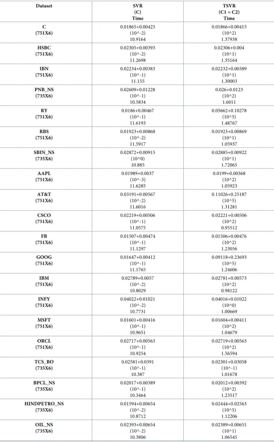
Table 3. Performance comparison of TSVR with SVR on individual companies’ stock datasets using a linear ker-nel. RMSE is used for comparison. Time is used for the training in seconds.

Dataset SVR (C) Time TSVR (C1 = C2) Time C (751X6) 0.01865+0.00425 (10^-2) 10.9164 0.01866+0.00415 (10^2) 1.37938 HSBC (751X6) 0.02305+0.00393 (10^-2) 11.2698 0.02306+0.004 (10^1) 1.35164 IBN (751X6) 0.02234+0.00383 (10^-1) 11.155 0.02232+0.00389 (10^1) 1.30003 PNB_NS (735X6) 0.02609+0.01228 (10^-1) 10.5834 0.026+0.0123 (10^2) 1.6011 RY (751X6) 0.0186+0.00467 (10^-1) 11.6193 0.05662+0.10278 (10^5) 1.48767 RBS (751X6) 0.01923+0.00868 (10^-2) 11.5917 0.01923+0.00869 (10^1) 1.05937 SBIN_NS (735X6) 0.02872+0.00915 (10^0) 10.885 0.02885+0.00922 (10^1) 1.72065 AAPL (751X6) 0.01989+0.0037 (10^-3) 11.6285 0.0199+0.00368 (10^2) 1.05923 AT&T (751X6) 0.03191+0.00567 (10^-2) 11.6016 0.11026+0.25187 (10^5) 1.31281 CSCO (751X6) 0.02219+0.00506 (10^-1) 11.0575 0.02221+0.00506 (10^2) 0.95512 FB (751X6) 0.01507+0.00474 (10^-1) 11.1297 0.01506+0.00476 (10^2) 1.23056 GOOG (751X6) 0.01647+0.00412 (10^-1) 11.1765 0.09118+0.23693 (10^5) 1.24606 IBM (751X6) 0.02789+0.0057 (10^-2) 10.8029 0.02781+0.00573 (10^2) 0.98122 INFY (751X6) 0.04022+0.01021 (10^-2) 10.7731 0.04016+0.01022 (10^0) 1.00669 MSFT (751X6) 0.01601+0.00416 (10^-1) 10.9651 0.01604+0.00411 (10^2) 1.04679 ORCL (751X6) 0.02717+0.00563 (10^-1) 10.9254 0.02719+0.00563 (10^2) 1.56594 TCS_BO (735X6) 0.02581+0.0391 (10^-1) 10.387 0.02301+0.03058 (10^-1) 1.01678 BPCL_NS (735X6) 0.02017+0.00389 (10^-1) 10.3464 0.02012+0.00392 (10^2) 1.23517 HINDPETRO_NS (735X6) 0.01594+0.00654 (10^-2) 10.8712 0.02444+0.02563 (10^5) 1.12206 OIL_NS (735X6) 0.02393+0.00654 (10^-2) 10.3806 0.02389+0.00651 (10^1) 1.06545 (Continued)

whereFFis the distribution according to theF-distribution and (1,1×23) = (1, 23) is the degree of freedom. Here, 4.2793 is the critical value ofF(1,23) for the level of significance atα= 0.05. Since the value ofFF= 11.8632>4.2793, we reject the null hypothesis. Furthermore, we per-formed pairwise comparisons using the Nemenyi post hoc test of all reported methods and veri-fied the significant difference between their average ranks by computing the critical difference (CD) atp= 0.10. The difference between their ranks should be at least1:645

ffiffiffiffiffiffiffiffiffiffiffi 2�ð2þ1Þ

6�24

q

�0:3358. Since the difference between the average ranks of TSVR with SVR (1.791667−1.208333 = 0.583334) is greater than 0.3358, we conclude that TSVR is significantly better than SVR for individual stock datasets. For the non-linear case, the absolute prediction error of SVR and

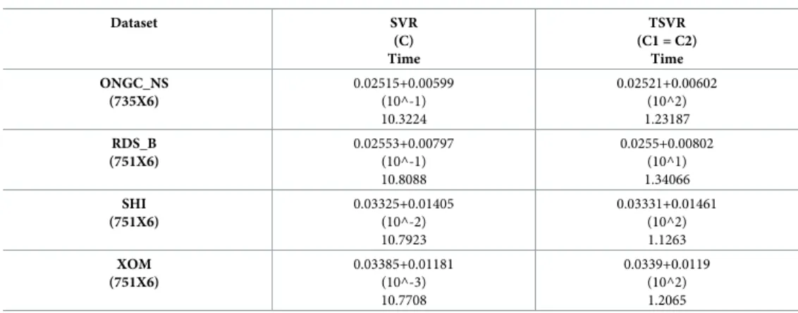
Table 3. (Continued) Dataset SVR (C) Time TSVR (C1 = C2) Time ONGC_NS (735X6) 0.02515+0.00599 (10^-1) 10.3224 0.02521+0.00602 (10^2) 1.23187 RDS_B (751X6) 0.02553+0.00797 (10^-1) 10.8088 0.0255+0.00802 (10^1) 1.34066 SHI (751X6) 0.03325+0.01405 (10^-2) 10.7923 0.03331+0.01461 (10^2) 1.1263 XOM (751X6) 0.03385+0.01181 (10^-3) 10.7708 0.0339+0.0119 (10^2) 1.2065 https://doi.org/10.1371/journal.pone.0211402.t003

Fig 1. Prediction error plots using a linear kernel on the SHI dataset.

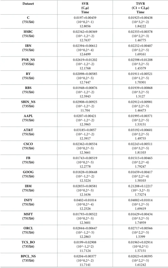
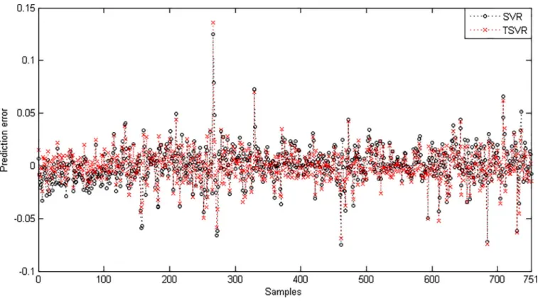
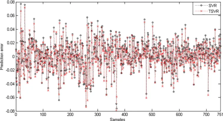
TSVR is shown in Figs3and4for the FB and RY datasets, respectively. Additionally, the actual and predicted values of SVR and TSVR are plotted in Figs5and6for the FB and RY datasets, respectively. It can easily be observed that TSVR is in close agreement with the observed values compared to SVR.

Stock market index datasets

Stock market index datasets such as BSESN and HSI consist of 733 closing prices, while DJI and IXIC have 751 closing prices; the FCHI and IBEX datasets consist of 763 closing prices; the JKSE and TWII datasets consist of 724 closing prices; MXX and SSMI have 750 closing points; AEX consists of 763 closing points; ATX consists of 737 closing points; BFX consists of 762 closing points; BVSP consists of 738 closing points and GDAXI, GSPTSE, KS11, N225, NSEI, STOXX50E consist of 755, 748,728, 732, 731, 745 closing points, respectively, from 01-01-2015 to 31-12-2017. The current value is predicted by using the previous five closing prices.

Linear case. For the linear kernel,Table 6shows the average RMSE for the optimal parame-ter values with the standard deviation and the training time in seconds. We can conclude that TSVR gives better results in 13 cases out of 20 datasets in terms of average RMSE of test accuracy. Additionally, the training time of TSVR is lower than that of SVR. The Friedman statistical non-parametric post hoc test is performed on the average rank of 20 financial datasets fromTable 7. The Friedman statistic [40] can be computed under the null hypothesis for the linear case:

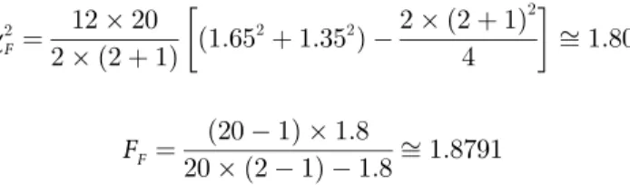
w2 F¼ 12�20 2� ð2þ1Þ ð1:65 2 þ1:352 Þ 2� ð2þ1Þ 2 4 � � ffi1:80 FF¼ ð20 1Þ �1:8 20� ð2 1Þ 1:8ffi1:8791

whereFFis distributed according to theF-distribution with (1,19), which has the critical value

4.3807 for the level of significanceα= 0.05. Here,FFis less than the critical value, so there is no

significant difference between these two algorithms for the linear case.Fig 7shows the absolute prediction error plot of SVR and TSVR for the linear kernel on the BFX dataset.Fig 8also shows the actual and predicted values of SVR and TSVR for the linear kernel on the market stock index BFX dataset. One can easily conclude that TSVR is in close agreement with the target values compared to SVR.

Nonlinear case. For the non-linear kernel,Table 8shows the average RMSE for the opti-mal parameter value with the standard deviation and the training time in seconds. We can conclude that TSVR gives better results in 19 out of 20 datasets in terms of average RMSE of test accuracy. The training time of TSVR is less than that of SVR due to solving a pair of smaller-sized QPPs instead of a large QPP, as in the case of SVR. This shows the superiority of TSVR with respect to SVR.

In the nonlinear case for different stock market index datasets, the Friedman statistic can be computed under the null hypothesis fromTable 7as:

w2 F¼ 12�20 2� ð2þ1Þ ð1:95 2 þ1:052 Þ 2� ð2þ1Þ 2 4 � � ffi16:2 FF¼ ð20 1Þ �16:2 20� ð2 1Þ 16:2ffi81

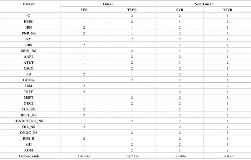
Table 4. Average ranks of TSVR with SVR on individual companies’ stocks using a linear and Gaussian kernel.

Dataset Linear Non-Linear

SVR TSVR SVR TSVR C 1 2 2 1 HSBC 1 2 1 2 IBN 2 1 2 1 PNB_NS 2 1 2 1 RY 1 2 2 1 RBS 2 1 2 1 SBIN_NS 1 2 1 2 AAPL 1 2 2 1 AT&T 1 2 1 2 CSCO 1 2 2 1 FB 2 1 2 1 GOOG 1 2 2 1 IBM 2 1 1 2 INFY 2 1 2 1 MSFT 1 2 2 1 ORCL 1 2 2 1 TCS_BO 2 1 2 1 BPCL_NS 2 1 2 1 HINDPETRO_NS 1 2 2 1 OIL_NS 2 1 2 1 ONGC_NS 1 2 2 1 RDS_B 2 1 2 1 SHI 1 2 2 1 XOM 1 2 1 2 Average rank 1.416667 1.583333 1.791667 1.208333 https://doi.org/10.1371/journal.pone.0211402.t004

Table 5. Performance comparison of TSVR with SVR on individual companies’ stock datasets using a Gaussian kernel. RMSE is used for comparison. Time is used for the training in seconds.

Dataset SVR (C,μ) Time TSVR (C1 = C2,μ) Time C (751X6) 0.0197+0.00459 (10^0,2^-1) 12.8056 0.01925+0.00438 (10^3,2^-2) 1.84222 HSBC (751X6) 0.02342+0.00369 (10^-1,2^-2) 12.7637 0.02355+0.00378 (10^2,2^-3) 1.46775 IBN (751X6) 0.02394+0.00612 (10^0,2^-4) 12.6499 0.02252+0.00407 (10^2,2^-5) 1.69161 PNB_NS (735X6) 0.02619+0.01202 (10^-1,2^-2) 12.1768 0.02598+0.01208 (10^3,2^-5) 1.45579 RY (751X6) 0.02098+0.00585 (10^0,2^-5) 12.7447 0.01911+0.00521 (10^1,2^-5) 1.70301 RBS (751X6) 0.01948+0.00876 (10^-1,2^-2) 12.5943 0.01939+0.00868 (10^3,2^-5) 1.5127 SBIN_NS (735X6) 0.02908+0.00925 (10^-1,2^-2) 11.704 0.02912+0.00981 (10^2,2^-5) 1.46473 AAPL (751X6) 0.0207+0.00421 (10^-1,2^-2) 12.3965 0.01995+0.00371 (10^2,2^-5) 1.53151 AT&T (751X6) 0.03185+0.0057 (10^-1,2^-2) 12.3917 0.03192+0.00601 (10^2,2^-5) 1.49755 CSCO (751X6) 0.02362+0.00534 (10^0,2^-5) 12.3661 0.02243+0.00511 (10^3,2^-5) 1.81103 FB (751X6) 0.01743+0.00519 (10^0,2^-5) 12.2778 0.01515+0.00465 (10^2,2^-4) 1.79247 GOOG (751X6) 0.01828+0.00648 (10^-1,2^-2) 12.3224 0.01659+0.00417 (10^2,2^-4) 1.50103 IBM (751X6) 0.02855+0.00581 (10^0,2^-5) 12.1636 0.21208+0.12217 (10^-3,2^-3) 1.73274 INFY (751X6) 0.0402+0.01014 (10^0,2^-4) 12.2526 0.04002+0.01014 (10^1,2^-5) 1.69419 MSFT (751X6) 0.01793+0.00522 (10^0,2^-5) 12.3601 0.01629+0.00434 (10^3,2^-5) 1.74959 ORCL (751X6) 0.02844+0.00647 (10^-1,2^-5) 12.2863 0.02717+0.00566 (10^2,2^-5) 1.5399 TCS_BO (735X6) 0.0199+0.02908 (10^-1,2^2) 11.7124 0.01963+0.02914 (10^0,2^1) 1.57151 BPCL_NS (735X6) 0.0204+0.00377 (10^0,2^-2) 11.7141 0.02023+0.00395 (10^2,2^-5) 1.61242 (Continued)

whereFFis the distribution according to theF-distribution with (1,1×19) = (1,19) as the degree of freedom. Here, 4.3807 is the critical value ofF(1,19) for the level of significance atα= 0.05. Since the value ofFF= 81>4.3807 is rejected, we reject the null hypothesis. Similar to the previ-ous case, we perform pairwise comparisons using the Nemenyi post hoc test for all reported

Table 5. (Continued) Dataset SVR (C,μ) Time TSVR (C1 = C2,μ) Time HINDPETRO_NS (735X6) 0.01869+0.00916 (10^1,2^-4) 11.8947 0.01607+0.00664 (10^3,2^-3) 1.52778 OIL_NS (735X6) 0.02512+0.00797 (10^0,2^-2) 11.7162 0.02407+0.0067 (10^2,2^-5) 1.63295 ONGC_NS (735X6) 0.02644+0.00678 (10^-1,2^-4) 11.7554 0.02581+0.00658 (10^2,2^-5) 1.37471 RDS_B (751X6) 0.02737+0.01047 (10^-1,2^-4) 12.3922 0.02587+0.00841 (10^1,2^-5) 1.48654 SHI (751X6) 0.03433+0.01577 (10^-1,2^-4) 12.3041 0.03366+0.01511 (10^2,2^-5) 1.45092 XOM (751X6) 0.03391+0.01177 (10^0,2^-4) 12.3424 0.03395+0.01186 (10^2,2^-5) 1.7403 https://doi.org/10.1371/journal.pone.0211402.t005

Fig 3. Prediction error plots using a Gaussian kernel on the FB dataset.

Fig 4. Prediction error plots using a Gaussian kernel on the RY dataset.

https://doi.org/10.1371/journal.pone.0211402.g004

Fig 5. Predicted and actual values using a Gaussian kernel on the FB dataset.

Fig 6. Predicted and actual values using a Gaussian kernel on the RY dataset.

https://doi.org/10.1371/journal.pone.0211402.g006

Table 6. Performance comparison of TSVR with SVR on stock market index datasets using a linear kernel. RMSE is used for comparison. Time is used for the training in seconds.

Dataset SVR (C) Time TSVR (C1 = C2) Time AEX (763X6) 0.02683+0.01051 (10^-1) 11.8233 0.02678+0.01061 (10^5) 1.47306 ATX (737X6) 0.01886+0.00414 (10^-2) 10.3641 0.01885+0.0043 (10^1) 1.1216 BFX (762X6) 0.03424+0.01144 (10^-1) 11.3085 0.03545+0.01039 (10^3) 1.16305 BSESN (733X6) 0.02062+0.00448 (10^-1) 10.2492 0.02071+0.00445 (10^1) 1.22084 BVSP (738X6) 0.01993+0.00365 (10^-2) 10.4724 0.01997+0.00379 (10^2) 0.97825 DJI (751X6) 0.01413+0.00492 (10^-1) 10.8441 0.01419+0.0048 (10^2) 1.39238 FCHI (763X6) 0.03166+0.01213 (10^-2) 11.1665 0.03159+0.01216 (10^2) 0.93741 (Continued)

methods and verify the significant critical difference between their average ranks. The differ-ence between their ranks should be at least1:645

ffiffiffiffiffiffiffiffiffiffiffi 2�ð2þ1Þ

6�20

q

�0:3678atp= 0.10.

Since the difference between the average ranks of TSVR with SVR (1.95−1.05 = 0.90) is greater than 0.3678, we conclude that TSVR is significantly better than SVR for stock market index datasets. For the non-linear case, the absolute prediction error of SVR and TSVR is shown in Figs9,10and11for the BVSP, DJI and IXIC datasets, respectively. The actual and predicted values of SVR and TSVR are plotted in Figs12,13and14for the BVSP, DJI and IXIC datasets, respectively. It can easily be observed from these figures that TSVR is in close

Table 6. (Continued) Dataset SVR (C) Time TSVR (C1 = C2) Time GDAXI (755X6) 0.02591+0.00872 (10^-2) 10.8492 0.02586+0.00873 (10^1) 1.12026 GSPTSE (748X6) 0.02208+0.00768 (10^-1) 10.6209 0.02214+0.00779 (10^2) 1.28185 HSI (733X6) 0.02125+0.00607 (10^-2) 10.2733 0.0212+0.00608 (10^1) 1.26684 IBEX (763X6) 0.02829+0.00918 (10^-2) 11.1037 0.02828+0.0091 (10^1) 1.44011 IXIC (751X6) 0.0165+0.00475 (10^-1) 10.8561 0.01645+0.00473 (10^2) 1.10158 JKSE (724X6) 0.01871+0.0053 (10^-1) 10.4427 0.18938+0.36737 (10^5) 1.19995 KS11 (728X6) 0.02053+0.00366 (10^-2) 10.1628 0.02052+0.00367 (10^2) 0.90443 MXX (750X6) 0.03059+0.00594 (10^-1) 10.6947 0.03052+0.006 (10^1) 1.47527 N225 (732X6) 0.02757+0.01059 (10^-1) 10.2778 0.02753+0.01071 (10^1) 1.14582 NSEI (731X6) 0.01992+0.00419 (10^-1) 10.1286 0.01994+0.00419 (10^1) 1.18078 SSMI (750X6) 0.0402+0.0164 (10^-1) 10.8077 0.04008+0.01626 (10^1) 1.32179 STOXX50E (745X6) 0.032+0.01324 (10^-2) 10.5735 0.03193+0.01327 (10^1) 1.1432 TWII (724X6) 0.02051+0.00474 (10^-1) 10.0368 0.02049+0.00477 (10^2) 1.23588 https://doi.org/10.1371/journal.pone.0211402.t006

Table 7. Average ranks of TSVR with SVR on stock market index datasets using a linear and Gaussian kernel.

Dataset Linear Non-Linear

SVR TSVR SVR TSVR AEX 2 1 2 1 ATX 2 1 2 1 BFX 1 2 2 1 BSESN 1 2 2 1 BVSP 1 2 2 1 DJI 1 2 2 1 FCHI 2 1 2 1 GDAXI 2 1 2 1 GSPTSE 1 2 2 1 HIS 2 1 2 1 IBEX 2 1 2 1 IXIC 2 1 2 1 JKSE 1 2 2 1 KS11 2 1 2 1 MXX 2 1 2 1 N225 2 1 2 1 NSEI 1 2 2 1 SSMI 2 1 1 2 STOXX50E 2 1 2 1 TWII 2 1 2 1 Average rank 1.65 1.35 1.95 1.05 https://doi.org/10.1371/journal.pone.0211402.t007

Fig 7. Prediction error plots using a linear kernel on the BFX dataset.

Fig 8. Predicted and actual values using a linear kernel on the BFX dataset.

https://doi.org/10.1371/journal.pone.0211402.g008

Table 8. Performance comparison of TSVR with SVR on stock market index datasets using a Gaussian kernel. RMSE is used for comparison. Time is used for the training in seconds.

AEX (763X6) 0.02765+0.01023 (10^0,2^-2) 12.781 0.02698+0.0106 (10^2,2^-5) 1.73396 ATX (737X6) 0.01949+0.00416 (10^-1,2^-2) 11.907 0.01892+0.00422 (10^2,2^-5) 1.41487 BFX (762X6) 0.03466+0.01048 (10^-2,2^-1) 12.787 0.03395+0.0117 (10^2,2^-5) 1.40597 BSESN (733X6) 0.02264+0.00551 (10^0,2^-2) 11.8247 0.02073+0.00453 (10^3,2^-4) 1.56612 BVSP (738X6) 0.0222+0.00447 (10^-1,2^-5) 11.9909 0.02005+0.00391 (10^2,2^-5) 1.43526 DJI (751X6) 0.01721+0.00561 (10^0,2^-5) 12.3971 0.0155+0.00503 (10^2,2^-5) 1.74354 FCHI (763X6) 0.03171+0.01203 (10^-1,2^-2) 12.6618 0.03156+0.01218 (10^2,2^-5) 1.53077 GDAXI (755X6) 0.02662+0.00822 (10^-1,2^-2) 12.4439 0.02601+0.00867 (10^2,2^-5) 1.49756 GSPTSE (748X6) 0.02627+0.0173 (10^-1,2^-2) 12.2009 0.02301+0.00875 (10^3,2^-5) 1.44924 (Continued)

agreement with the desired output in comparison to SVR, which clearly demonstrates the applicability and usefulness of TSVR.

Conclusion

In this paper, support vector regression and twin support vector regression formulations are discussed in detail and applied to an individual companies’ stock indices in the area of information technology industries, banking, oil, and petroleum industry and stock market index datasets of different countries to predict stock prices. Here, a pair of smaller sized QPPs is solved instead of a single large sized QPP, as in the case of SVR, thus yielding a reduction in the cost of the system. To verify the effectiveness of TSVR, we performed numerical experiments for both linear and Gaussian kernels on financial time series data-sets. In experimental results, TSVR shows better learning speed for both linear and Gauss-ian kernels with the ability to predict having a better generalization ability than SVR. In fact, the computation time of the TSVR is approximately four times lower than the stan-dard SVR in terms of learning speed, which clearly indicates its existence and usability. In future work, a new model that is able to handle noise and outliers for predicting the prices of stock indices can be explored.

Table 8. (Continued) HSI (733X6) 0.02189+0.00633 (10^-1,2^-2) 11.7218 0.02156+0.00623 (10^2,2^-5) 1.38225 IBEX (763X6) 0.0285+0.00925 (10^-1,2^-4) 12.6977 0.02842+0.00915 (10^2,2^-5) 1.47464 IXIC (751X6) 0.01906+0.00513 (10^0,2^-5) 12.3108 0.01681+0.0047 (10^2,2^-5) 1.69016 JKSE (724X6) 0.01922+0.00522 (10^0,2^-2) 11.3828 0.01893+0.00533 (10^2,2^-2) 1.57983 KS11 (728X6) 0.02197+0.00448 (10^-1,2^-4) 11.6135 0.02073+0.00373 (10^2,2^-5) 1.34512 MXX (750X6) 0.03145+0.00605 (10^0,2^-5) 12.4093 0.03082+0.0058 (10^2,2^-3) 1.73352 N225 (732X6) 0.02952+0.01077 (10^-1,2^-5) 12.0234 0.02839+0.01029 (10^2,2^-5) 1.3794 NSEI (731X6) 0.02206+0.00591 (10^-2,2^-1) 11.9166 0.02013+0.00444 (10^3,2^-5) 1.29858 SSMI (750X6) 0.04002+0.01628 (10^-1,2^-4) 12.3919 0.04007+0.0161 (10^2,2^-5) 1.42911 STOXX50E (745X6) 0.03218+0.01336 (10^0,2^-4) 12.4306 0.03204+0.01328 (10^2,2^-5) 1.66912 TWII (724X6) 0.02084+0.0046 (10^-1,2^-1) 11.495 0.02057+0.00472 (10^2,2^-5) 1.34332 https://doi.org/10.1371/journal.pone.0211402.t008

Fig 9. Prediction error plots using a Gaussian kernel on the BVSP dataset.

https://doi.org/10.1371/journal.pone.0211402.g009

Fig 10. Prediction error plots using a Gaussian kernel on the DJI dataset.

Fig 11. Prediction error plots using a Gaussian kernel on the IXIC dataset.

https://doi.org/10.1371/journal.pone.0211402.g011

Fig 12. Predicted and actual values using a Gaussian kernel on the BVSP dataset.

Fig 13. Predicted and actual values using a Gaussian kernel on the DJI dataset.

https://doi.org/10.1371/journal.pone.0211402.g013

Fig 14. Predicted and actual values using a Gaussian kernel on the IXIC dataset.

Author Contributions

Conceptualization: Deepak Gupta. Data curation: Deepak Gupta. Formal analysis: Mukesh Prasad.

Funding acquisition: Mahardhika Pratama. Investigation: Deepak Gupta.

Supervision: Jun Li.

Validation: Mahardhika Pratama, Mukesh Prasad. Visualization: Mukesh Prasad.

Writing – original draft: Deepak Gupta.

Writing – review & editing: Mahardhika Pratama, Zhenyuan Ma, Jun Li, Mukesh Prasad.

References

1. Vapnik VN. (2000). The nature of statistical learning theory, 2nd ed., Springer, New York

2. Osuna E, Freund R, Girosi F. (1997). Training support vector machines: An application to face detec-tion, in Proceedings of Computer Vision and Pattern Recognidetec-tion, 130–136

3. Huang C, Davis LS, Townshed JRG. 2002. An assessment of support vector machines for land cover classification. International Journal of Remote Sensing, 23, 725–749.

4. Joachims T. (1998). Text categorization with support vector machines: learning with many relevant fea-tures, In: European Conference on Machine Learning No.10, Chemnitz, Germany, 137–142

5. Brown MPS, Grundy WN, Lin D, Cristianini N, Sugnet CW, Furey TS, et al. (2000), Knowledge-based analysis of microarray gene expression data using support vector machine, Proceedings of the National Academy of Sciences of USA, 97(1), 262–267

6. Guyon I, Weston J, Barnhill S, Vapnik V. (2002). Gene selection for cancer classification using support vector machine, Machine Learning, 46, 389–422

7. Mukherjee S, Osuna E, Girosi F. (1997). Nonlinear prediction of chaotic time series using support vector machines, In: NNSP’97: Neural Networks for Signal Processing VII: in Proc. of IEEE Signal Processing Society Workshop, Amelia Island, FL, USA, 511–520

8. Muller KR, Smola AJ, Ratsch G, Scho¨lkopf B, Kohlmorgen J. (1999). Using support vector machines for time series prediction, In: Scho¨lkopf B, Burges CJC, Smola AJ (Eds.), Advances in Kernel Methods-Support Vector Learning, MIT Press, Cambridge, MA, 243–254

9. Lin F, Yeh C, Lee M. (2011). The use of manifold learning and support vector machines in the prediction of business failure, Knowledge-Based Systems, 24(1), 95–101

10. Boser BE, Guyon IM, Vapnik VN. (1992). A training algorithm for optimal margin classifiers. In proceed-ings of the Annual Conference on Computational Learning Theory, Haussler D, Ed., ACM Press, Pitts-burgh, PA, pp. 144–152

11. Joachims T. (1999). Making large-scale SVM learning practical. In Advances in Kernel Methods—Sup-port Vector Learning, Sch¨olkopf B, Burges CJC, Smola AJ, Eds., MIT Press, Cambridge, MA, pp. 169–184,

12. Platt J. (1999). Fast training of support vector machines using sequential minimal optimization. In Advances in Kernel Methods—Support Vector Learning, Sch¨olkopf B., Burge C.J.C., and Smola A.J., Eds., pp. 185–208, MIT Press, Cambridge, MA

13. Achlioptas D, McSherry F, Sch¨olkopf B. (2002). Sampling techniques for kernel methods, In Advances in Neural Information Processing Systems 14, Dietterich T. G., Becker S., and Ghahramani Z., Eds., MIT Press, Cambridge, MA.

14. Fine S, Scheinberg K. (2001). Efficient SVM training using low-rank kernel representations, Journal of Machine Learning Research, 2:243–264

15. Tsang IW, Kwok JT, Cheung PM. (2005). Very large SVM training using core vector machines. In pro-ceedings of the Tenth International Workshop on Artificial Intelligence and Statistics, Barbados.

16. Suykens JAK, Vandewalle J. (1999). Least squares support vector machine classifiers. Neural Process-ing Letters, 9(3), 293–300.

17. Suykens JAK, Lukas L, Van DP, Moor BD, Vandewalle J. (1999). Least squares support vector machine classifiers: a large scale algorithm, European Conference on Circuit Theory and Design, (ECCTD’99), Stresa Italy, pp.839-842.

18. Mangasarian OL, Wild EW. (2006). Multisurface Proximal Support Vector Classification via Generalized Eigenvalues, IEEE Transaction on Pattern Analysis and Machine Intelligence, 28(1), 69–74.

19. Jayadeva KR, Chandra S. (2007). Twin support vector machines for pattern classification, IEEE Trans-action on Pattern Analysis and Machine Intelligence (TPAMI), 29, 905–910.

20. Peng X (2010a). TSVR: An efficient twin support vector machine for regression, Neural Networks, 23 (3), 365–372

21. Emad WS, Danil VP, and Donald CW. (1998). Comparative study of stock trend prediction using time delay, recurrent and probabilistic neural networks, IEEE Trans. on Neural Networks, 9(6): 1456–1470. https://doi.org/10.1109/72.728395PMID:18255823

22. Cao L, Tay FEH. (2001) Financial forecasting using support vector machines, Neural Computing and Application, 10: 184–192.

23. Kuo RJ, Chen CH, Hwang YC. (2001) An intelligent stock trading decision support system through inte-gration of genetic algorithm based fuzzy neural network and artificial neural network, Fuzzy Sets and Systems, 118(1): 21–45.

24. Prasad M, Li DL, Lin CT, Singh J, Prakash S. (2015). Designing Mamdani-Type Fuzzy Reasoning for Visualizing Prediction Problems Based on Collaborative Fuzzy Clustering. IAENG International Journal of Computer Science, 42 (4).

25. Singh J, Prasad M, Prasad OK, Er MJ, Saxena A, Lin CT. (2016). A Novel Fuzzy Logic Model for Pseudo Relevance Feedback based Query Expansion. International Journal of Fuzzy Systems, 18 (6), 980–989.

26. Prasad M, Liu YT, Li DL, Lin CT, Shah RR, Kaiwartya OP. (2016). A New Mechanism for Data Visualiza-tion with TSK-type Preprocessed Collaborative Fuzzy Rule based System. Journal of Artificial Intelli-gence and Soft Computing Research.

27. Prasad M, Lin YY, Lin CT, Er MJ. (2015). A New Data-Driven Neural Fuzzy System with Collaborative Fuzzy Clustering Mechanism. Neurocomputing, 167, 558–568, 2015.

28. Lin CT, Prasad M, Saxena A. (2015). An Improved Polynomial Neural Network Classifier Using Real Coded Genetic Algorithm. IEEE Transaction on Systems, Man and Cybernetics: Systems, 45 (11), 1389–1401.

29. Prasad M, Lin CT, Hong CT, Chang JY. (2017). Soft Boosted Self Constructive Neuro Fuzzy Inference Network. IEEE Transaction on Systems, Man and Cybernetics: Systems, 47 (3), 584–588.

30. Kim KJ, Han I. (2000). Genetic algorithms approach to feature disctetization in artificial neural networks for the prediction of stock price index, Expert Systems with Applications, 19: 125–132.

31. Hassan MR, Nath B. (2005). Stock market forecasting using hidden Markov model: a new approach, Proc. 5th International Conference on Intelligent Systems Design and Applications, 192–196.

32. Fama EF, Kenneth RF. Dividend yields and expected stock returns. Journal of financial economics 22.1 (1988): 3–25.

33. Lewellen J. "Predicting returns with financial ratios." Journal of Financial Economics 74.2 (2004): 209– 235.

34. Goh JC, Jiang F, Tu J, Wang Y. Can US economic variables predict the Chinese stock market?. Pacific-Basin Finance Journal 22 (2013): 69–87.

35. Shen D, Zhang Y, Xiong X, Zhang W. Baidu index and predictability of Chinese stock returns. Financial Innovation (2017) 3:4.

36. Xiao L, Shen D, Zhang W. "Do Chinese internet stock message boards convey firm-specific informa-tion?" Pacific-Basin Finance Journal 49 (2018): 1–14.

37. Pissarenko D. (2002). Neural networks for financial time series prediction: Overview over recent research BSc (Hones) Computer Studies Thesis, University of Derby in Austria.<http://citeseer.ist.psu. edu/pissarenko02neural.html>.

38. http://finance.yahoo.com

39. http://www.mosek.com

40. Demsˇar J. Statistical comparisons of classifiers over multiple data sets. Journal of Machine learning research 7.Jan, pp. 1–30 (2006).