Learning Action-State Representation Forests for Implicitly Relational Worlds

(1)

UNIVERSITY OF OKLAHOMA GRADUATE COLLEGE

LEARNING ACTION-STATE REPRESENTATION FORESTS FOR IMPLICITLY RELATIONAL WORLDS

A DISSERTATION

SUBMITTED TO THE GRADUATE FACULTY in partial fulfillment of the requirements for the

Degree of DOCTOR OF PHILOSOPHY By THOMAS J. PALMER Norman, Oklahoma 2015

(2)

LEARNING ACTION-STATE REPRESENTATION FORESTS FOR IMPLICITLY RELATIONAL WORLDS

A DISSERTATION APPROVED FOR THE SCHOOL OF COMPUTER SCIENCE

BY

Dr. Andrew H. Fagg, Chair

Dr. Dean F. Hougen

Dr. S. Lakshmivarahan

Dr. Amy McGovern

Dr. David P. Miller

(3)

(4)

(5)

Acknowledgments

First, I’d like to thank the people directly involved in this work. This includes Andy Fagg, of course, for his mentoring and great support over the years. I’d also like to thank my other committee members for their contributions: Dean Hougen, S. Lakshmivarahan, Amy McGovern, Dave Miller, and Rick Thomas. Also, thanks go to Matt Bodenhamer for the SMRF project that I build on here. Thanks also to Dan Fennelly, Dougal Sutherland, and Sam Bleckley, other students who have worked on SMRF. Other students in the Symbiotic Computing Laboratory have also helped out a lot in my time here, including Di Wang, Josh Southerland, and Kim Houck, including in reviewing this document.

A lot of other folks at OU have also been good support in various roles, including professors Deborah Trytten, Sridhar Radhakrishnan, and John Antonio. Fellow student coworkers in TA and instructor roles have also been great. Among various folks in the CS office, I’d like to thank Barbara Bledsoe, Chyrl Yerdon, Emily Pierce, Jaime Hoots, Lisa Moore, and Virginie Perez Woods. Y’all are great! I’d also like to thank the students I’ve taught at OU, and my friends in CSGSA have also been awesome. I’m still leaving out way too many people, but thanks anyway, y’all.

Also, during a substantial portion of my time at OU, I’ve been supported by a University of Oklahoma Foundation Fellowship. I appreciate that support im-mensely.

I should also acknowledge all my friends from Los Alamos and White Rock that make it seem like getting a PhD is a normal thing. And I’d like to thank folks at Eyefinity for sending me off with well wishes, and thanks also to Mike Goodrich at BYU and other faculty and fellow students who supported me there and whom I

(6)

still count among my friends.

Of course, I also need to thank my amazing wife, Kristine, who let me come back to school and who never stopped believing in me. Our kids have put up with a lot because of this, too, so I’d like to thank each of them: Jacob, David, Sam, Anna, Zeke, and Lydia. Thanks also to Kristine’s and my parents and many other family members for their support. I’ve been enough trouble, but they haven’t stopped putting up with me.

(7)

List of Tables

3.1 Summary of synthetic multiple instance learning (MIL) data sets. . . 35 3.2 Mean PSS, using constant/heuristic parameter choices for each

learn-ing method. . . 38 3.3 Mean PSS, using SVM parameters chosen by grid search. . . 39 3.4 Mean training and prediction time in seconds, using constant/heuristic

(10)

List of Figures

3.1 Overview of the learning process. . . 28

4.1 Hand-crafted SMRF tree. . . 43

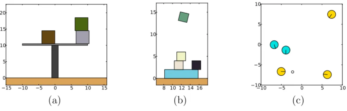
5.1 Example starting states for the three tasks evaluated. . . 57

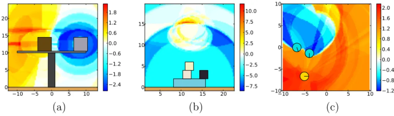
5.2 SVM decision values showing sample evaluations for the three exper-imental tasks. . . 58

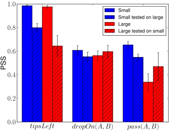
5.3 Mean and standard deviation of classification performance. . . 60

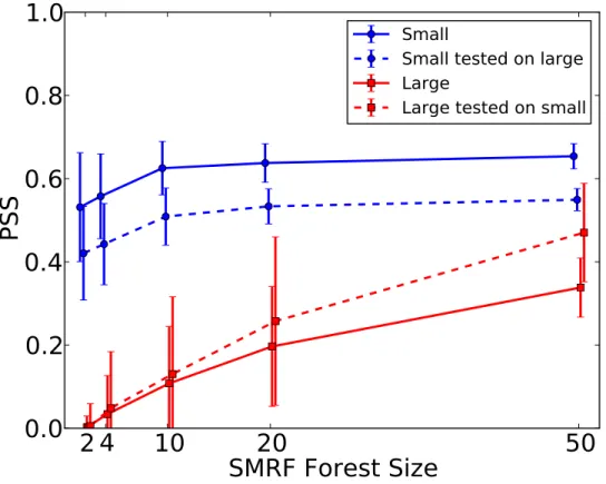
5.4 Mean and standard deviation of performance as a function of forest size. . . 62

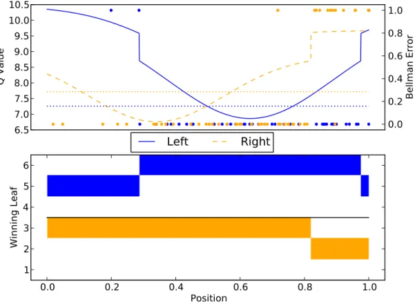
6.1 SMRF-RPI policy for 1D corridor task. . . 71

7.1 SMRF-RPI policy for 1D corridor task. . . 79

7.2 Reward for different episode counts for corridor task. . . 80

7.3 Reward for bits and densities for corridor task. . . 81

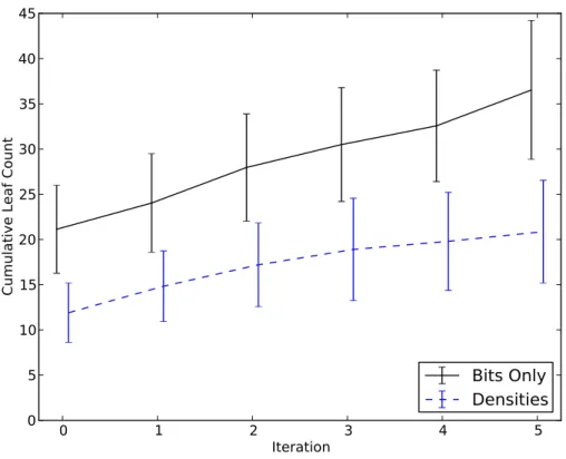
7.4 Cumulative leaf count for bits and densities for corridor task. . . 82

7.5 Examples episodes for the high towers task. . . 86

7.6 Example tree forput(A, B) on the high towers task. . . 88

7.7 Example tree for “not”rotate(A) on the high towers task. . . 89

7.8 Reward for high towers task. . . 90

7.9 Examples episodes for the color grouping task. . . 94

7.10 Example tree for put(A, B) on the CIEDE2000 color grouping task. . 95

7.11 Example tree for “not”isolate(A) on the CIEDE2000 color grouping task. . . 96

7.12 Reward for the CIEDE2000 color grouping task. . . 97

7.13 Reward for the RGB color grouping task. . . 99

7.14 Cumulative leaf counts for the CIEDE2000 and RGB color grouping tasks. . . 100

7.15 Example arch with scored area. . . 101

7.16 Examples episodes for the arch building task. . . 104

7.17 Example tree for done on the arch task. . . 105

7.18 Reward for arch building task. . . 107

7.19 Slices of example policy learned by SMRF-RPI for the keepaway task. 110 7.20 Example tree for “not” pass(A, B) on the keepaway task. . . 111

7.21 Reward for SMRF-RPI and CMAC Sarsa at 50 episodes per iteration. 113 7.22 Reward for SMRF-RPI and CMAC Sarsa at 500 episodes per itera-tion. . . 114

7.23 Sarsa learning results for SMRF and CMAC representations. . . 116

(11)

7.25 Reward and cumulative leaf count for various configurations of SMRF-RPI. . . 119 7.26 Reward and cumulative leaf count for various configurations of

SMRF-RPI. . . 120 A.1 Example tree forput(A, B) on the high towers task for a second RPI

iteration. . . 140 A.2 Example tree forrotate(A) on the high towers task for a second RPI

iteration. . . 141 A.3 Example tree for “not” done on the arch building task for a second

RPI iteration. . . 142 A.4 Example tree for “not” move(A, B) on the arch building task for a

second RPI iteration. . . 144 A.5 Example tree forrotate(A) on the arch building task for a third RPI

iteration. . . 145 A.6 Example tree for done on the arch building task for a third RPI

iteration. . . 146 A.7 Example tree for “not” move(A, B) on the arch building task for a

third RPI iteration. . . 147 A.8 Example tree for “not” hold(A) on the keepaway task for a second

RPI iteration. . . 148 A.9 Example tree for “not” pass(A, B) on the keepaway task for a second

(12)

List of Algorithms

2.1 Least Squares Temporal Difference Q-learning (LSTDQ) . . . 13

2.2 Least Squares Policy Iteration (LSPI) . . . 13

2.3 Generic Representation Policy Iteration (RPI) using LSTDQ . . . 16

3.1 Covariant Aggregation . . . 27

4.1 SMRF Learning Algorithm . . . 46

4.2 SMRF Leaf Probability Assignment . . . 49

(13)

Abstract

Real world tasks, in homes or other unstructured environments, require interacting with objects (including people) and understanding the variety of physical relation-ships between them. For example, choosing where to place a fork at a table requires knowing the correct position and orientation relative to the plate. Further, the quantity of objects and the roles they play might change from one occasion to the next; the variables are not fixed and predefined. For an intelligent agent to navigate this complex space, it needs to be able to identify and focus on just those variables that are relevant. Also, if a robot or other artificial agent can learn such physical relations from its own experience in a task, it can save manual engineering effort and automatically adapt to new situations.

Relational learning, while often focused on discrete domains, applies to situations with arbitrary numbers of objects by using existential and/or universal quantifiers from first-order logic. The field of reinforcement learning (RL) addresses learning task execution from scalar rewards based on agent state and action. Relational reinforcement learning (RRL) combines these two fields.

In this dissertation, I present an RRL technique emphasizing relations that are merely implicit in multidimensional, continuous object attributes, such as position, color, and size. This technique requires analyzing permutations of possible object comparisons while simultaneously working in the multidimensional spaces defined by their attributes. Existing similar RRL methods query only one dimension at a time, which limits effectiveness when multiple dimensions are correlated.

Specifically, I present a representation policy iteration (RPI) method using the spatiotemporal multidimensional relational framework (SMRF) for learning

(14)

rela-tional decision trees from object attributes. This SMRF-RPI algorithm interleaves the learning of relational representations and of policies for agent action. Further, SMRF-RPI includes support for continuous actions. As a component of the SMRF framework, I also present a novel multiple instance learning (MIL) algorithm, which is able to learn parametric, existential decision volumes within a feature space in a robust manner.

Finally, I demonstrate SMRF-RPI on a variety of developmentally motivated blocks world tasks, as well as effective transfer and sample efficient learning in a standard keepaway soccer benchmark task. Both domains involve complicated, simulated world dynamics in continuous space. These experiments demonstrate SMRF-RPI as a promising method for applying RRL techniques in multidimen-sional, continuous domains.

(15)

Chapter 1 Introduction

The real world is a complicated place. For example, a robot working in an everyday kitchen needs to avoid obstacles, retrieve items, open containers, and combine and mix ingredients, among other activities. In these tasks, each action involves only a subset of the objects in the environment. When pouring flour into a bowl, the relative positions of the bowl and measuring cup are important. The pouring edge should be approximately centered above, but not too far above, the bowl. Other nearby objects might also interfere, but the exact locations of items on the spice shelf are probably irrelevant, and different objects might be present at different times. Some attributes of key objects also are likely irrelevant, such as the color of the bowl. For the objects and attributes that do matter, rather complicated world dynamics are at play, including gravity and the dispersion of flour in the air. The robot’s own developmental experience (see Fagg, 1993) can help it to form the concepts needed to successfully perform tasks such as these. For example, from its experience dropping of objects on each other, the robot can learn to interpret the world, for this specific kind of action, in terms of just the variables most likely to be relevant.

For an intelligent agent to learn to accomplish such tasks on its own, a num-ber of questions are salient. What high-level relations or predicates (such as over

or between) might exist in the raw physical data? Which are the key objects or

participants in a particular situation or scene? How should the agent behave to accomplish its task, and how do its actions affect the world? Learning discrete

(16)

predicates in a continuous space (such as for position or color) requires finding a meaningful decision volume in the space. Discovering which objects take on which roles requires iterating through permutations of possible assignments. Although it is computationally untenable to optimize across all possible solutions, an agent learning on its own still needs to answer these questions in an effective and efficient fashion.

A variety of research areas come to bear in answering these questions. Reinforce-ment learning (RL) addresses learning to perform multistep tasks, where the agent’s decision-making policy is defined by the outcome of each agent action, including a scalar reward signal, which might be positive or negative. Representation learning addresses the construction of features whereby to interpret the environment. Rela-tional learning addresses environments in which the relationships between multiple objects is important for making predictions or taking actions, and where the num-ber of objects might change in different situations. Relational concepts can be used as representations for task execution. For example, when considering passing the ball in a soccer game, I might care if there exists an opponent between me and a teammate. This concern is relevant no matter how many players are on the field. In first-order logic, this is called existential quantification. Relational learning might also address first-order universal quantification, which asks whether some property holds for all objects. For example, are all the appliances in the kitchen in work-ing order? Again, this question is meanwork-ingful no matter how many appliances are present.

Relational reinforcement learning (RRL) combines relational learning and rein-forcement learning (Blockeel and De Raedt, 1998; van Otterlo, 2005, 2012). RRL is ultimately concerned with how an agent should behave in relational worlds. How-ever, traditional relational learning methods do not emphasize continuous, multidi-mensional environments. Often, they rely on hand-crafted predicates (e.g., Pasula

(17)

et al., 2007) or query continuous variables in only one dimension at a time (e.g., Blockeel and De Raedt, 1998). These limitations can prove detrimental when mul-tiple dimensions are correlated. For example, the color yellow in the RGB color space requires covariance between the red and green color channels. Approximating a covariant volume with single dimensional queries may require numerous conjunc-tions. Methods that seek to learn relations that directly model multidimensional data sometimes do so without the ability to consider either existential or univer-sal quantification during the relation learning process (e.g., Kulick et al., 2013). These methods also commonly consider only binary relations, such as those based on relative positions of pairs of objects.

In this dissertation, I present a method for RRL that addresses multidimensional continuous variables in a fashion that is unique among relational learning systems. In this approach, I both utilize and contribute a key component to the spatiotempo-ral multidimensional relational framework (SMRF) of Bodenhamer (2014), which learns relations to answer existential questions. The SMRF learning algorithm builds a decision tree from binary-labeled samples, where each sample is a set of objects. Each object has associated real-valued, multidimensional attributes, such as position or color. Such attributes increase the complexity of relational learning, which must already address permutations of objects in the scene when considering their possible roles. Concerning permutations, Bodenhamer (2014) demonstrates SMRF’s effectiveness at pruning the search space when high numbers of irrelevant objects are present. Often, only a small fraction of object permutations needs to be considered. Bodenhamer also demonstrates that SMRF’s ability to learn decision volumes in multidimensional spaces can be more effective than working in individual dimensions, especially when covariance exists in the data.

The SMRF learning algorithm is a binary classifier that learns high-level relations (such as over or between) beginning from continuous object attributes. To do

(18)

this, the SMRF framework uses mapping functionsof the attributes of two or more objects to provide relative measures. As an example, a mapping function of relative position could provide a set of vectors corresponding to the relative positions of all pairs of objects in a scene. A relational existential question, such as whether any object exists above another, then becomes a question of which vectors are important among a set where most are irrelevant. The field of multiple instance learning (MIL) addresses this existential learning problem (Dietterich et al., 1997). In this dissertation, I contribute a novel multiple instance learning (MIL) algorithm called covariant aggregation, which includes direct support for covariance between dimensions. This algorithm is used for learning existential decision volumes within SMRF.

As a prelude and potential complement to relational reinforcement learning (RRL), I also present a learning method, using SMRF, to predict binary success or failure of actions. I approach this action outcome prediction in light of Gibsonian

affordances (Gibson, 1977); if an action is likely to be successful, then one might consider it as an affordance provided to the agent. In predicting outcomes, trees learned by SMRF provide representational features for other learning algorithms, such as support vector machine (SVM) classification or approximate reinforcement learning (e.g., Lagoudakis and Parr, 2003). Among these features, in a matter rem-iniscent of relational model trees (see, e.g., Vens et al., 2007), I also present a novel method for extracting continuous, radial features from SMRF trees.

For reinforcement learning, I apply a representation policy iteration (RPI) mech-anism (Mahadevan, 2005a), wherein representation learning is interleaved with pol-icy learning. Across RPI iterations, a forest of SMRF trees is built for each kind of action (e.g., placing one object on another vs. rotating an object). In my work, I also present a method for continuous actions, rather than considering only ac-tions parameterized on the discrete objects in a scene. My method for continuous

(19)

actions involves sampling possible actions as virtual objects. To summarize, key contributions of this dissertation include the following:

a novel multiple instance learning (MIL) algorithm, emphasizing support for covariant decision volumes and instance labeling, and which provides the method for learning decision volumes in SMRF;

an affordance-oriented method for relational learning to predict action success or failure in multidimensional, continuous domains;

an algorithm for relational reinforcement learning (RRL) in multidimensional, continuous domains, using a representation policy iteration (RPI) framework; a mechanism for automatic extraction of continuous, radial features from

SMRF trees;

demonstration of ternary mapping functions in continuous domains that con-sider the relative positions of three objects; and

demonstration of a mechanism for continuous actions in RRL.

In experimental evaluation, I minimally adapt parameters for the core learning sys-tem between different tasks. I test relational learning primarily in 2D simulated soccer and block stacking domains. In a keepaway soccer benchmark task (Stone et al., 2006), I show sample-efficient learning, compared to common, existing tech-niques. I also show effective transfer between tasks with different numbers of ob-jects/participants.

Going forward in this dissertation, Chapter 2 discusses related prior work, includ-ing the reinforcement learninclud-ing methods on which I base my work, and also discusses other relational reinforcement learning methods. Chapter 3 presents my covariant aggregation MIL algorithm. Chapter 4 discusses the SMRF relational tree learning

(20)

algorithm of Bodenhamer, which I use for relational learning in agent tasks, and to which I have contributed the MIL method for learning decision volumes. Chapter 5 presents my SMRF-forest-based method for binary action outcome prediction, in-cluding the use of ternary mapping functions. Chapter 6 presents my SMRF-RPI

method for RRL. This chapter also presents my method for extraction of continuous, radial features and also my method for support of continuous actions. Chapter 7 presents experimental results for the SMRF-RPI method. Chapter 8 discusses con-clusions and future work.

(21)

Chapter 2 Related Work

This work is primarily concerned with the learning of relational representations for reinforcement learning. Therefore, I first address the topic of reinforcement learning, with a focus on least squares policy iteration (Lagoudakis and Parr, 2003), a method for evaluating actions using linear approximation, given a feature basis for representing states and actions. My primary contribution in this dissertation is a technique for iteratively learning relational features using multidimensional object attributes to form such a basis for approximation. I therefore follow the discussion of approximate reinforcement learning with a review of representation learning and relational learning, especially as applied to relational reinforcement learning.

2.1 Reinforcement Learning

2.1.1 Markov Decision Processes and Q Learning

Multistep tasks occur regularly in daily life. Such tasks sometimes involve reaching a particular goal, such as in driving to work. Others involve maximizing some quantity, such as the amount of work performed during the day. An agent might also receive negative rewards (corresponding, perhaps, to costs or punishment) while working through a task. The reward framework adapts easily to goal-oriented tasks simply by, for example, providing positive reward for reaching a goal. Multistep tasks involving reward are often formulated as a Markov Decision Processes (MDPs), in which the current world state and agent action fully determine the probability

(22)

of next state and reward. That is, the MDP model assumes that the future is independent of the past, given the present. This assumption is called the Markov property. Formally, an MDP is a tuple of (S, A,P, R) where:

S is the set of states,

A is the set of actions available to the agent,

P(s0, s, a) = Pr (st+1 =s0|st =s, at=a) is the state transition function where

s0 ∈S, s∈S, a∈A, and t is the current time step, and

R(s0, s, a) = E[rt|st+1 = s0, st = s, at = a] is the expected reward function,

where rt is the reward at the state transition (Bellman, 1957a; Sutton and

Barto, 1998).

For MDPs, commonly, the goal is for the agent to learn policy:

π(s, a) = Pr (at =a|st=s)

such that expected long-term reward is maximized. Deterministic policies might be represented simply as functions fromS to A. The cumulative reward, or return, to be maximized could perhaps be the total reward for finite tasks or the discounted future reward for infinite horizon tasks. The latter option,

Rett=

∞

X

i=0

γirt+i,

is perhaps most common, whereγ ∈[0,1) is the reward discount factor.

More generally, actions can take arbitrary amounts of time. An MDP with tem-porally extended actions is called a Semi-Markov Decision Process (SMDP, Sutton et al., 1999), and such extended actions are calledoptions. In discrete-time SMDPs, options consist of a sequence of primitive actions where each primitive action takes

(23)

one time step. The reward for option o taken during agent experience at time t is merely the discounted sum of rewards for the individual actions in the sequence:

ro,t =

D−1

X

i=0

γirt+i,

where D is the duration of the option, and subsequent primitive actions or options are discounted as for D time steps in the future. For the sake of RL formalisms discussed in this section, I ignore the issue of temporally extended actions, as the discount modifications are straightforward.

For learning policies, different techniques exist. Forward planning (such as in Fikes and Nilsson, 1971) is a common technique to solve such tasks in ad hoc situ-ations. Another common technique is reinforcement learning (RL, see Sutton and Barto, 1998), which seeks to learn proper behavior for all situations based on past experience. RL is commonly based ondynamic programming(DP) theory (Bellman, 1957b). The learning process includes estimation of the values of states and state-action pairs. The value of a state for a given policy π gives the expected return for starting in state s and following π afterward:

Vπ(s) =E[Rett|st =s, π].

Making use of a state value function requires knowledge of P. That is, the agent needs to know which action leads to which next state in order to choose the best next state. On the other hand, by knowing the value of state-action pairs, it is possible to choose an action without explicit knowledge of future states. The Q function (Watkins and Dayan, 1992),

(24)

is the expected return for choosing action a in state s and following policy π after-ward. Given the MDP definitions for state transition and reward functions:

Qπ(s, a) = X s0 P(s0, s, a) R(s0, s, a) +γX a0 π(s0, a0)Qπ(s0, a0) ! . (2.1)

Techniques such as the popular Q-learning (Watkins and Dayan, 1992) are able to learn an optimal policyπ∗ for an MDP without explicitly modelingP. Indicating the Q function for π∗ as Q∗ and noting that π∗ always chooses the action that maximizesQ∗, Equation 2.1 becomes:

Q∗(s, a) =X s0 P(s0, s, a)R(s0, s, a) +γmax a0 Q ∗ (s0, a0).

Q∗ can be learned iteratively for finite states and actions during interaction with the world by the update rule:

Qt(s, a) = (1−αt)Qt−1(s, a) +αt rt+γmax a0 Qt−1(s 0 , a0),

where αt is the learning rate at time t. Given certain conditions on αt and

explo-ration,Qt converges in the limit to Q∗. The optimal policy then is:

π∗(s) = argmax

a

Q∗(s, a). (2.2)

2.1.2 Least Squares Policy Iteration

For discrete states and actions, given conditions onαt and repeated sampling of all

actions in all states, the Q learning algorithm converges in the limit to Q∗ and π∗ (Watkins and Dayan, 1992). However, for large or continuous state-action spaces, it might be infeasible to calculate an exact Q function. Standard function approxima-tion techniques can be applied in such cases; for an overview, see Sutton and Barto

(25)

(1998, Chapter 8).

One common method is to learn a linear combination of nonlinear features that capture sufficient information about the world:

b

Qπ(s, a) = φ(s, a)|wπ,

where φ(s, a) is a k ×1 vector of arbitrary features, and wπ, also a k-vector, is of

feature weights. The dimensions ofφ are presumed to be linearly independent.

One high-profile method for linearly weighted Q-learning is Least-Squares Temporal-Difference Q-learning (LSTDQ) of Lagoudakis and Parr (2003). For reinforcement learning in this dissertation, I use LSTDQ as well as the Least Squares Policy It-eration (LSPI) method (Lagoudakis and Parr, 2003) for iteratively bootstrapping feature weights from a fixed batch of experience. In the remainder of this section, I present an overview of these methods.

Assuming rewards don’t depend directly on next state, Equation 2.1 can be expressed as follows: Qπ(s, a) =R(s, a) +γ X s0_∈_S P(s0, s, a)X a0_∈_A π(s0, a0)Qπ(s0, a0).

For finite states and actions, this can be expressed in matrix form:

Qπ =R+γPΠπQπ,

whereQπ andRare column vectors of size|S||A|×1,Pis a matrix of size|S||A|×|S|

where:

(26)

and Ππ is a matrix of size |S| × |S||A| where:

Ππ(s,(s, a))) =π(s, a).

Then PΠπ is a matrix of size |S||A| × |S||A|, where the rows indicate the current

state and action, and columns indicate the next state and action. That is, if the agent is in a given state and takes a given action, what is the probability that it will be in a given next state and take the given next action? Rows ofP, Ππ, and PΠπ

each sum to 1.

As mentioned earlier, we can approximate Qπ by introducing abstract state

features, now in matrix form:

b

Qπ =Φwπ,

where Φ is a |S||A| ×k matrix of transposed feature vectors for every state and action. This approximation gives:

b

Qπ ≈ R+γPΠπQbπ and

Φwπ ≈ R+γPΠπΦwπ.

Note that choosing Φ as the identity matrix is equivalent to using original states and actions as the features for a finite state-action space.

Lagoudakis and Parr emphasize a least squares fixed-point solution to this sys-tem, which finds weights that minimize the distance betweenQbπ and R+γPΠπQbπ

using projection onto the space spanned by Φ:

Φwπ =Φ(Φ|Φ)

−1

(27)

Algorithm 2.1 Least Squares Temporal Difference Q-learning (LSTDQ)

procedure LSTDQ(D, k, φ, γ, π) . D is a bag of data samples from any agent

behavior. e A←0k×k eb←0_k×1 for (s, a, r, s0)∈D do e A←Ae +φ(s, a) φ(s, a)−γφ s0, π(s0)| eb←eb+φ(s, a)r end for e wπ ←Ae−1eb returnw_eπ end procedure

Algorithm 2.2 Least Squares Policy Iteration (LSPI) procedure LSPI(D, k, φ, γ, , w0) w0 ←w0 repeat w←w0 w0 ←LSTDQ(D, k, φ, γ, πw) untilkw−w0k< returnw end procedure

This yields the solution:

wπ = (Φ|(Φ−γPΠπΦ))

−1

Φ|R.

To express that some states and actions have greater importance or are visited more frequently than others, a diagonal weighting matrix ∆µ may be included (which is

equivalent to nonorthogonal projection):

wπ = (Φ|∆µ(Φ−γPΠπΦ))

−1

Φ|∆µR.

The above solution requires an enumeration of all states and actions, whether or not they are encountered. It also requires knowledge of P. Alternatively, the following components can be approximated iteratively over examples from actual

(28)

agent experience:

A = (Φ|_∆

µ(Φ−γPΠπΦ)) , and

b = Φ|∆µR,

wherewπ =A−1b. Algorithm 2.1 shows the LSTDQ algorithm, which approximates

these components (as Ae−1 andeb) and calculates w_π. Finally, Algorithm 2.2 shows

the Least Squares Policy Iteration (LSPI) algorithm for bootstrapping policy learn-ing from a fixed set of examplesD. Each iteration of LSTDQ provides a new policy, which in turn affects the next calculation of A. Here,e w₀ contains initial weights,

which might be zero, small random values, or based on prior learning, if any, and is a cutoff level to test for approximate convergence.

2.2 Representation Learning

In reinforcement learning, linear approximations ofQπ depend intimately on feature

space φ(s, a). Features could be manually specified in a domain-dependent fashion, or perhaps in a somewhat generic form such as polynomials, radial basis functions, overlapping tilings (Sutton and Barto, 1998), or cosine waves (Konidaris et al., 2011). Alternatively, features can be automatically derived from knowledge of the task space or learned from agent experience.

Feature selection and construction are both common concerns in the general field of machine learning (Guyon and Elisseeff, 2003), not just for representations for RL. Feature selection assumes an existing set of features, some of which might be better for the task at hand than others. Many selection techniques are classi-fied as either filter methods, operating before the primary learning mechanism is used, or else wrapper methods, selecting features by testing the performance of the primary learner given different feature subsets. Feature construction assumes that the best representation might be (possibly nonlinear) functions of one or more of

(29)

the originally available features. Newly constructed features might be aggregated to the existing set, increasing dimensionality, or they might be used to replace ex-isting features, possibly decreasing dimensionality (such as for principle component analysis). Also, the recent explosion in deep learning methods (Bengio, 2009), build-ing on older work such as multilayer artificial neural networks (Hornik et al., 1989; Schmidhuber, 2015), is largely concerned with the topic of feature construction.

2.2.1 Feature Construction for RL

Early work in automatic feature or basis function construction specifically for rein-forcement learning includes the Proto-Value Functions (PVFs) of Mahadevan (2007), which generates basis functions from the state adjacency matrix. Another common technique is to build functions based on the Bellman error (BE) of the current Q function (Parr et al., 2008; Wu and Givan, 2010). For any particular example of agent experience

BE =r+γQπ(s0, a0)−Qπ(s, a). (2.3)

As earlier discussed, the Bellman error is 0 in expectation for the correct Qπ.

Fea-tures constructed in this fashion are sometimes called Bellman Error Basis FeaFea-tures (BEBFs). Mahadevan and Liu (2010) shows that BEBFs converge slowly for highγ and suggests the use of Bellman Average Reward Bases (BARBs) as an alternative. Features can also be constructed based on actual agent performance (Girgin and Preux, 2008b). The techniques above are immediately useful to LSPI, although it is worth noting that feature learning techniques also exist that are more directly tied to other RL methods (e.g., Girgin and Preux, 2008a; Kersting and Driessens, 2008). Finally, feature selection (in addition to construction) is also a concern in RL (for example, Kolter and Ng, 2009).

(30)

Rep-Algorithm 2.3 Generic Representation Policy Iteration (RPI) using LSTDQ procedure RPI(γ, , w0)

repeat

Gather agent experience D.

Learn representation φ, whose dimensionality is k.

w0 ←w0

repeat

w←w0

w0 ←LSTDQ(D, k, φ, γ, πw)

Optionally adapt the basis. until kw−w0k<

untilconverged, if desired returnw

end procedure

resentation Policy Iteration (RPI) by Mahadevan (2005b). Although, in his work, he primarily focuses on particular forms of basis function construction, this framework is applicable to a full variety of techniques, as discussed above. I give a modified RPI overview in Algorithm 2.3. When using LSTDQ, the inner loop of RPI is very similar to LSPI, except with the added optional step for basis adaptation. Ma-hadevan also leaves the outer loop optional, and other small variations also exist in different presentations of the framework. Within my present work, I use the term RPI generally to mean any interleaving of representation and policy learning.

2.3 Relational Reinforcement Learning

2.3.1 Relational Learning

In many real-world contexts, multiple objects exist with relationships between each other. For example, a plate could be on a table, or one person might be standing between two others. Such contexts are often described via first-order logic. For example:

(31)

expresses that there exists at least one plate such that is on the table, which, here, is presumed to be a constant. First-order logic, which includes quantifiers∃ and ∀, differs from propositionallogic, which operates on fixed constants.

Logical quantifiers loop over possible objects in a scene. Importantly, the number of objects in a scene might not be constant from one situation to the next. This is often touted as a benefit of relational learning over propositional learning, where

relational also is often taken to mean first-order (Blockeel and De Raedt, 1998; Dˇzeroski et al., 2001). This same perspective consideres traditional machine learning algorithms, operating on vectors of fixed length, to be propositional.

TILDE

While much of the field of Inductive Logic Programming (ILP; see Muggleton, 1991; De Raedt and Kersting, 2008) includes some amount of first-order logical learning, the most relevant alternative to my present work is the TILDE (Top-down Induction of Logical Decision Trees) algorithm of Blockeel and De Raedt (1998). TILDE recursively builds a decision tree, choosing query nodes that maximize some metric (such as information gain) with respect to the training examples and background knowledge. Each training example is a graph with objects and propositions giving information about them, including relations between objects.

The types of queries available are manually given in the form of refinement specifications. These specifications indicate how many variables may be introduced, which may be reused from existing variables, which predicates can be used, and so on. Further, manual lookahead specifications allow multiple queries to be introduced at the same time (Blockeel and De Raedt, 1997), which otherwise is prohibited due to exponential growth in the search space. For example, when playing soccer, it might be relevant that an opponent is nearby. However, that someplayer is nearby might not be very meaningful on its own, and that some player is an opponent

(32)

might also be meaningless for making a decision, without also emphasizing where that player is. However, asking all pairs (or more) of questions in a row without having some meaningful distinctions made along the way is a deep search problem. Therefore, a lookahead specification might be given to allow asking about team membership followed by specific kinds of questions about location.

Free variables are implicitly existentially quantified. A querysucceedsif it has at least one true binding of constants to the variables. A recursive query down a tree follows only one path, so if a query fails, it means that there exists no binding. In this fashion, TILDE also supports universal quantifiers, although negative forms of predicates need to be explicitly specified to allow positive universals. For example, to say that all parts of a machine are working, a specification needs to be given to allow asking that a part is notworking, and a query can then test that there exists no broken part. That is, the query would fail, and the example would proceed down the negative branch, thus saying that all parts are in working order.

Core TILDE works with discrete data rather than with continuous values. There-fore, continuous values must be discretized into bins before learning a tree or query-ing an existquery-ing one (Blockeel and De Raedt, 1997). TILDE usually determines thresholds in a supervised fashion based on information entropy in the training set. For multidimensional attributes (e.g., position in 3D space), each dimension is discretized as a separate variable, and a single query can also ask about only one dimension. Multiple queries down a single branch a required to carve a volume in multidimensional space.

TILDE has also been used for regression, in a batch-learning algorithm called TILDE-RT (Blockeel et al., 1998) or an incremental version called TG (Driessens et al., 2001). For TILDE regression, each scene has a single real-valued label. Each leaf has a value which is the prediction for scenes arriving there. In learning, the goal is typically to minimize mean squared error. Queries are selected that minimize

(33)

this, where leaf values are selected as the mean of values of the scenes arriving at them. Finally, ReMauve (Vens et al., 2007) is a variation that allows for linear regression in the leaves by selecting aggregate or single values from the constants bound to variables in a tree.

Other Relational Learning Approaches

As mentioned above, a variety of other relational learning systems exist. Most notable for my present work is the Spatiotemporal Multidimensional Relational Framework (SMRF) of Bodenhamer (2014), which I use for relational learning for the methods presented in this dissertation. SMRF is a decision tree framework that operates directly on multidimensional continuous attributes, as opposed to the discretization and single-dimensional approach of TILDE. SMRF has also been shown to handle large numbers of distractor objects better. I cover this framework in detail in Chapter 4.

Additionally, a large body of work also exists in the field of Multiple Instance Learning (MIL), which most commonly addresses simple existential questions in multidimensional continuous spaces. As demonstrated by Bodenhamer (2014), such algorithms can be applied to pairwise relational learning problems, again by creating instances as pairs of existing objects, with attributes as relative measures. I address MIL in more detail in Chapter 3.

2.3.2 Combining Relational Learning with Reinforcement Learning As relational learning inherently addresses worlds with variable numbers of objects, much work exists in the use of relational representations for reinforcement learning (van Otterlo, 2005, 2012). Of course, relational planning mechanisms are one of the traditional foci in artificial intelligence (e.g., Fikes and Nilsson, 1971).

(34)

typi-cally centered on variations around Q-learning. As seen earlier, learning the Q func-tion allows policy learning without explicit modeling of the state following agent action. From a relational perspective, one common Q-learning strategy is to employ relational regression methods to approximate the Q function as experience increases. One of the seminal works in this field is the relational reinforcement learning work of Dˇzeroski et al. (2001). This work uses TILDE-RT, where each training example con-sists of (si, ai, qi), and eachqi =ri+γmaxa0Qˆ_j(s_i₊₁, a0), in standard fashion. The Q

function is subscripted here by experience iteration j. Specifically, the agent gath-ers a batch of experience based on current function Qj, and this generates learning

examples as described. With each new batch of examples, TILDE-RT learns a new tree. After the first iteration, each new batch is aggregated to prior examples. Each old example has its associated qi updated to match the latest Qj. Using the entire

set of examples, a new tree is learned which replaces the old tree. This provides the Q-RRL algorithm. Dˇzeroski et al. (2001) also present the P-RRL algorithm which learns an additional tree predicting the policy directly and generalizes better to environments where the Q function itself might be inconsistent.

Later work in this vein employs other relational regression algorithms in addi-tion to incremental variaaddi-tions on the algorithms using TG (Driessens et al., 2001). When incremental, each new MDP sample (s, a, s0, r) can be immediately used for updating the Q function. Other relational regression algorithms employed includ-ing relational instance-based regression (RIB) of Driessens and Ramon (2003) and the TRENDI method of Driessens and Dˇzeroski (2005), which learns trees via TG, but uses RIB in the leaves rather than a constant mean value. The kernel-based relational regression (KBR) method of G¨artner et al. (2003) uses graph kernels and Gaussian processes for Q-function regression. Kersting and Driessens (2008) dif-fer in learning relational trees (using TG) to follow a probabilistic policy gradient; Natarajan et al. (2011) use this same method for imitation learning. Wu and Givan

(35)

(2010) use a beam search through relational expressions finding those that corre-late with Bellman error within a representation policy iteration framework. Jetchev et al. (2013) use a relational nearest neighbor approach to learn grounded symbols for MDP planning techniques. Zaragoza and Morales (2009) employ an RRL sys-tem for robot navigation that discretizes state and action space but also constructs continuous actions by interpolation. Many other techniques for RRL have also been employed (van Otterlo, 2012).

Of note, across these techniques, while various algorithms other than trees have been introduced for RRL, tree learning, and especially TILDE in various forms, is one of the common methods that continues to be employed, suggesting its ver-satility and effectiveness. However, as noted, SMRF has been shown to be more effective than TILDE in multidimensional, continuous domains for binary classifi-cation (Bodenhamer, 2014), but prior to my current work, it has not been used for reinforcement learning.

2.3.3 Other Continuous, Relation-Oriented Task Learning

Of note beyond model-free RRL, other planning and RL techniques exist for con-tinuous, multidimensional tasks of a relational nature. Some are relational in the first-order sense, and some merely consider physical relations without support for quantifiers. Some emphasize learning of abstract predicates and symbols, and others use human-designed, high-level representations.

One notable work in relational MDPs for continuous tasks is that of Pasula et al. (2007), which employs human-designed predicate representations of a 3D physics-based, simulated block-stacking domain. Their algorithm learns rules predicting the outcomes of actions, thus yielding a relational model useful for MDP planning. Lang and Toussaint (2010) explore more advanced planning algorithms built atop models learned by the method of Pasula et al. (2007). Kulick et al. (2013) continue this

(36)

work, learning specific relations as noted earlier, working from simulated and real robot action. They work from specific pairs of objects, though, rather than being concerned with quantification when learning relations. Of note, they also include an action with a continuous parameter (not associated with an actually present object), but this action is used only for active learning and not for relational task planning. Mugan and Kuipers (2009), Modayil and Kuipers (2008), and Konidaris et al. (2014) also learn symbolic grounding of various sorts from multidimensional, con-tinuous data, but only in propositional form. Mugan and Kuipers (2009) is also an example of the field of Qualitative Reasoning (QR), which focuses on the use of high-level representation for perhaps otherwise continuous values. QR can include first-order relational work as well (for example Zhang and Renz, 2014). Xu and Laird (2011) learn symbolic, relational rules and also continuous, non-relational ac-tion models, fusing informaac-tion from the two in making predicac-tions about acac-tion outcomes.

As yet another and much different approach, Verbancsics and Stanley (2010) use the evolutionary HyperNEAT learning algorithm with a grid-based representation, where objects in the scene are marked onto the grid. This inherently supports an arbitrary number of objects in the grid, although the technique has a different nature than the set-based approach of standard relational representations.

(37)

Chapter 3 Multiple Instance Learning via Covariant Aggregation

A primary concern in relational learning is identifying the objects that play partic-ular roles. For example, in soccer, does there exist an opponent between me and the teammate to which I want to pass the ball? Such an opponent has the role of a potential interceptor, and the opponent has this role because of the physical relationship of being between me and my teammate. There are other players on the field who do not have this role. Mathematically, calculating the positions of all opponents relative to me and my teammate yields a set of vectors, and only those vectors within a particular region represent potential interceptors. In learning how to play, I need to determine what is in common between the cases where I make a successful pass as opposed to when I lose control of the ball.

This becomes an existential binary classification problem, commonly called a multiple instance learning (MIL) problem. For the larger relational setting, many relationships might need considered. Is there someone between the passer and the receiver? Is an opponent near the ball? Are multiple opponents nearby? Each such question becomes a MIL classification problem, and the specific nature of the layout of vectors for each question might vary. We might also want to ask more than one question about the same players or objects. Also, because of the multidimensional nature of physical attributes, it is possible that correlation exists between multiple dimensions. These are among the concerns at hand in solving the MIL problem for the relational tasks of interest in this dissertation. Therefore, in this chapter, I contribute a novel MIL algorithm for learning simple, covariant decision volumes

(38)

which performs robustly and quickly in a variety of example MIL data sets, without parameter tuning to each case.

3.1 Introduction

Machine learning, including classification, usually addresses inputs of individual, fixed-length feature vectors. In contrast, multiple instance learning (MIL) addresses unordered sets or bags of instances, where each instance is commonly a feature vector (Dietterich et al., 1997). Binary MIL classification problems commonly consider a bagpositiveif it has at least one instance that is a positive example of some concept; in other words, at least one instance is in a positive region of the vector space. In this formulation, MIL is an existential classification problem:

positive(B) =∃x∈Bpositive(x), (3.1)

where B is a bag, and each x is an instance. MIL therefore goes beyond ordinary vector-based learning, in that the learning algorithm must identify relevant instances while also learning to classify them. It also therefore provides a foundation for existential relational learning, as will be further discussed in Chapter 4.

Common examples of MIL include that of molecule classification, where each molecule has a set of potential foldings, and any one of those foldings might signify the key behavior of the molecule. Image classification is another example, where the task is to identify whether or not an image contains a particular object, given a bag of visual features, where it does not matter where an object is in the image or if other objects are present. A third example, relevant to relational task learning within the scope of this dissertation, in playing a game of soccer, passing a ball is likely to fail if there exists an opponent between the passer and the potential receiver; positions of other opponents might be less relevant.

(39)

Early MIL algorithms include axis-parallel rectangles (APR) of Dietterich et al. (1997) and diverse density (DD) of Maron and Lozano-P´erez (1997). APR greedily selects discriminating features, choosing minimum and maximum bounds for each feature value to ensure that at least one instance from each positive bag is included. DD defines a probabilistic metric emphasizing instances with many positive and few negative bags nearby. Using the DD metric, gradient ascent selects the best central feature vector and the scaling for each feature. Many other MIL algorithms and multiple-instance problem formulations (beyond just existential queries) have since been developed (see Foulds and Frank, 2010). These include such concerns as bag distance metrics and MIL-oriented kernels and constraints for support vector machines. While many of these techniques are often quite effective, learned models are not always intuitively clear to humans. Further, some techniques, including DD and APR, label individual instances as positive or negative, while others focus exclusively on labeling each bag as a whole.

In our work, we seek to determine instance labels, as well as to provide a simple description of the relevant volume in the feature space, such as those provided by APR and DD. However, neither APR nor DD acknowledge covariance that can occur across features. Covariance can arise, for example, in color models (such as yellow in RGB space, which contains equal parts red and green) or in spatial configurations (where interesting cases have some object along a particular vector). In MIL, simply realigning data to principal components is not ideal, as the representative instances might align very differently than the aggregate set of instances from positive bags. While Zhao et al. (2013) address learning of covariant distance metrics within MIL, they focus neither on simple decision volumes nor instance classification. Most similar to our own work is the recent work of Kandemir and Hamprecht (2014), who learn a Gaussian mixture model for MIL instance prediction using a Bayesian formulation. In this chapter, we present a learning technique that directly addresses

(40)

the learning of simple, covariant decision volumes for instance label prediction, and we show that our method is robust across a variety of learning problems without parameter tuning.

In the remainder of this chapter, we describe our MIL algorithm, which learns a covariant decision volume via iterative aggregation of volume-describing instances from positive bags. We then evaluate our method, on both synthetic and real-world data sets, against other well-known algorithms (including DD) that either describe ellipsoidal regions or else use radial feature kernels.

3.2 Learning Algorithm

We follow the common existential, instance-classifying MIL formulation established in Equation 3.1. In this form, the classifier’s job is to classify individual instances. If any instance in a bag is found to be positive, then the bag itself is labeled as positive.

The differentiating aspect of our approach is that of covariant decision volumes. This contrasts with the axis-aligned volumes of APR and DD. Specifically, we de-scribe a decision volume by its mean µ, covariance V, and radius r. Parameters µ and V provide the Mahalanobis distance from the volume center:

DM(x|µ, V) =

p

(x−µ)T_V−1₍_x₋_µ_). _(3.2)

Any instance x within radiusr is considered positive:

positive(x|µ, V, r) ⇐⇒ DM(x|µ, V)≤r. (3.3)

Throughout our discussion, we treat instances as feature vectors within a Eu-clidean topology. As such, we also refer to instances aspoints.

(41)

We now describe an algorithm for learning covariant decision volumes from train-ing data with labeled bags. Algorithm 3.1 gives informal pseudocode for the learntrain-ing process, and Figure 3.1 shows several steps of the process using a synthetic data set in which positive bags are more likely to have at least one instance along the diago-nal. In summary, our algorithm seeks a set ofkey points,K, from which to estimate parametersµand V. This process begins with a single key point from one sampled positive bag. At each iteration, the algorithm chooses a new key point from an unrepresented positive bag to add to this set, where the candidate key point from a bag is its point nearest to the current decision volume center (by Equation 3.2), also called the bag’switness point. Given the new potential set of key points,µand V are reestimated, and a new radius,r, is chosen to maximize the training accuracy (similar to the method of Auer and Ortner, 2004). Key point aggregation continues while training set accuracy across recent iterations suggests possible improvement.

In the remainder of this section, we elaborate on each step of the algorithm.

3.2.1 Covariance Estimation

Our algorithm determines a covariant, ellipsoidal decision volume starting from a single key point. Additional key points are aggregated iteratively. We calculate µ as the mean of the key points. However, when there are few key points relative to the dimensionality, covariance V is poorly defined. To condition the covariance, we begin with an inverse Wishart prior based on all points from all positive bags. The inverse Wishart distribution is conjugate prior to the multivariate covariance matrix (see Gelman et al., 2013). That is, given additional observations defining a covariance matrix, the posterior distribution is still inverse Wishart.

The inverse Wishart distribution has two parameters: a scale matrix, Ψ, and degrees of freedom, ν. The matrix Ψ represents a prior observation of covariance

(42)

Algorithm 3.1 Covariant Aggregation Begin set K with one initial key point.

Let BR be all positive bags not containing initial point.

Estimate µand V from K.

LetWbe witness points of minDM(x|µ, V) for all bags.

Choose radius r to maximize training set accuracy. Remember (µ, V, r) as initial best.

while progress continues do

LetBS be M sampled bags from BR.

for all B inBS do

LetK0 be K ∪ the witness point from W forB. Determine µ0, V0, W0, and r0 using K0.

Evaluate training accuracy for K0. end for

UpdateK, µ,V,W, and r for best B sampled. UpdateBR to exclude best B.

if new training accuracy ≥ previous best then Remember new best (µ, V, r).

end if end while

Return best (µ, V, r).

scaled by ν presumed observations. The posterior Ψpost is given by:

Ψpost = ncov(X) + Ψ

where

ncov(X) = (X−E[X])(X−E[X])T (3.4) is a scale matrix based on observations as column vectors in the matrix X.

Usually, the magnitude of the posterior covariance depends on the sum ofν and the number of new observations. However, in our case, we use our estimate of V only for the shape and orientation of the decision volume. Radius r is determined at a later step.

Also, because our learning problem is multiple-instance, there is no necessary relationship between all instances from positive bags and the final decision volume.

(43)

4 3 2 1 0 1 2 3 4 4 3 2 1 0 1 2 3 4 0.46 0.48 0.50 0.52 0.54 0.56 0.58 0.60 0.62 0.64

(a) Initial key point, with training set accuracy by radius. 4 3 2 1 0 1 2 3 4 4 3 2 1 0 1 2 3 4

(b) Radius with optimal accuracy.

4 3 2 1 0 1 2 3 4 4 3 2 1 0 1 2 3 4

(c) Decision volume after four key points. 4 3 2 1 0 1 2 3 4 4 3 2 1 0 1 2 3 4

(d) At 24 key points, the final decision volume.

Figure 3.1: Overview of the learning process. Circles indicate points from positive bags, and squares indicate negatives. Pale circles indicate key points. Larger mark-ers indicate witness points: the nearest point from each bag, given the current mean and covariance.

Therefore, we treat the weight of the prior as independent of both the number of bags and the number of instances. Instead, we use a hand-selected parameter, w, to influence the overall weight of the prior. Our effective posterior covariance is therefore:

Vpost= ncov(K) +wncov(P)/p, (3.5)

whereK represents the key points and P represents all points (quantityp) from all positive bags. Figures 3.1(a) and 3.1(b) show an initial covariance based entirely

(44)

on the prior, while Figures 3.1(c) and 3.1(d) show how an increasing number of key points can increasingly change the volume shape.

However, the covariance could still be poorly conditioned, especially in situations of high dimensionality. If the condition number of the covariance matrix is above a particular threshold c, we add a constant diagonal to this covariance:

V =        Vpost if max Λ_{min Λ} ≤c

Vpost+max Λ_c−₋c₁min ΛI otherwise,

(3.6)

where Λ is the set of eigenvalues of Vpost, and I is the identity matrix. This yields

a covariance matrix with a maximum condition number of c.

3.2.2 Decision Volume Radius

To choose decision volume radius r, we follow the optimal ball algorithm of Auer and Ortner (2004). Specifically, we select the radius that maximizes classification accuracy across all bags in the training set. Because each bag is classified as to whether any of its points lie within the decision volume, only the nearest point to the volume center is of interest. This nearest point is called thewitness pointfor its bag. We differ from Auer and Ortner primarily in our use of Mahalanobis distance. Formally, our set of witness points W is defined as:

W = argmin x∈B DM(x|µ, V) B ∈ B , (3.7)

where B represents all training bags (both positive and negative).

To choose radius r, we first sort W by increasing distance, and then perform a linear scan for maximal accuracy, also as suggested by Auer and Ortner. Fig-ure 3.1(a) illustrates training set accuracy as a function of radius, and FigFig-ure 3.1(b) shows the corresponding radius maximizing accuracy.

(45)

3.2.3 Key Point Aggregation

Before the outer loop of Algorithm 3.1, the algorithm samples a single positive bag. For each point in the bag, using only the covariance prior asV, a radius is chosen to maximize training accuracy. Iterative covariant aggregation, shown in Figure 3.1, begins from the point yielding highest accuracy.

At each aggregation step, the algorithm samples M positive bags currently un-represented among the key points, where M is an algorithm parameter. Further, to keep the search localized, only bags whose witness points lie inside the current decision volume are sampled, where, as suggested in Figure 3.1, the set of candidate bags changes as the volume changes. The witness point (and no others) from a sampled bag is tentatively added to the key points, and a new decision volume is constructed. Among sampled bags, the tentative key point set with highest accuracy is selected, and the aggregation process repeats.

Early in the search process, with few key points, the decision volume’s shape is very flexible. It becomes more established as the number of key points increases. Therefore, to terminate the aggregation process, we make a linear least squares estimate of training accuracy over the most recent A aggregation steps, whereA is an algorithm parameter. We continue aggregation if the accuracy slope is positive and if, continuing the current slope through remaining positive bags, the accuracy would surpass the previous best (including across restarts, as discussed shortly). Otherwise, aggregation stops, retaining the model with the highest accuracy. If decision volumes at multiple iterations have equal accuracy, we select the one with the most key points, as this presumably better describes the volume. At minimum, a full window of A iterations is required before termination.

As is common for stochastic algorithms, we restart the learning process multiple times. After each aggregation process, we sample another positive bag for the next

(46)

restart. Algorithm parameter N determines the number of restarts. Of the N resulting models, the volume with the highest accuracy with respect to the training set (or, again, in case of a tie, the one with the most key points) is selected as the final volume.

3.3 Experimental Evaluation

We test our method on two types of data sets: (1) synthetic data in two or three dimensions, of which some exhibit covariant regions of interest (discussed below), and (2) standard third-party MIL data sets, which usually have high dimensionality and do not necessarily exhibit interesting covariance.

We compare against other algorithms with ellipsoidal decision boundaries or ellipsoidal kernels. Techniques with ellipsoidal boundaries include the non-boosted optimal ball algorithm of Auer and Ortner (2004), and the DD (Maron and Lozano-P´erez, 1997) and EM-DD (Zhang and Goldman, 2001) algorithms. None of these are capable of expressing covariance, although DD and EM-DD scale original axes. We use the Weka (Hall et al., 2009) implementations of these algorithms with default parameters.

We also compare against SVM techniques mi-SVM, MI-SVM (Andrews et al., 2002), and MILES (Chen et al., 2006). For mi-SVM and MI-SVM, we use (isotropic) RBF kernels, and the MILES feature set is also based on a radially decaying measure. All three are therefore capable of expressing arbitrarily nonlinear surfaces, including approximations of covariance. Unlike other techniques compared here, MILES is a bag-only classifier rather than an instance classifier, but we include it because it is simple and performs well. We use the MISVM package of Doran and Ray (2014) for implementations of mi-SVM and MI-SVM. We use our own implementation of the MILES feature set with LIBLINEAR (Fan et al., 2008) as the SVM classifier,

(47)

using the L2-loss L1-regularization option, which differs from the L1-loss of standard MILES.

In testing the algorithms, we are primarily concerned with performance “in the wild.” That is, we assume that new learning problems need to be addressed without the opportunity for extensive analysis and parameter tuning. We therefore hold all parameters constant for our learning algorithm. Specifically, we hold constant the progress window size A at 8, covariance prior weight w at 10−1_{, max covariance}

condition c at 105_{, and both number of restarts} _N _{and number of aggregation}

bags sampled M at 4. We have chosen these parameters based upon exploratory investigations with some of the synthetic data sets, as well as the well-known Musk 1 data set (Dietterich et al., 1997).

Using a similar amount of exploration, we have also selected parameters C and γ for evaluation of SVM-based techniques. For C, we use a constant value of 104_.

We choose γ = 1_/₂_σ2 _{using a heuristic calculation for} _σ _{as the mean of the tenth}

and ninetieth percentiles of all (positive and negative) inter-point distances in the training set (e.g., as used as a starting point by Takeuchi et al., 2006).

Also, in exploration with DD and EM-DD, we found it necessary to filter the Musk data sets for meaningful learning results. Specifically, we divide the values of each feature dimension by their standard deviation. For consistency, we do this for all data sets for DD and EM-DD. We have not performed such filtering for other learning methods, although mechanisms such as the inverse Wishart prior used by our method provide a similar effect.

For our synthetic data sets, in addition to the heuristically-chosen SVM param-eters, we also test against tuned SVM parameters. In these cases, we search across a grid of C values from 10−4 to 109 (stepping by powers of 10) and factors of our heuristically-chosen γ, from 2−7 _{to 2}7_.

(48)

and/or stochastic learning than those used during exploratory evaluation or param-eter selection.

3.3.1 Synthetic, Low-Dimensional Data Sets

Our method is designed for use in low-dimensional (often physical) settings with potentially covariant classification volumes. We have therefore designed multiple synthetic learning problems that exhibit interesting characteristics in two or three dimensions. Summarized in Table 3.1, these data sets consist of the following mix-ture distributions:

Covariant 1, depicted in Figure 3.1, is a 2D problem where negative instances come from one of two isotropic Gaussians of standard deviation 1 and means of (−2,2) and (2,−2), respectively. Positive instances come from a covariant Gaussian along the orthogonal diagonal, centered at (0,0). Eigenvalues of the positive distribution are 1 and 1/52. All bags have 3 instances, where exactly 1 of the 3 is drawn from the positive distribution for each positive bag. Covariant 2 is the same as Covariant 1, except that there is a single

nega-tive distribution, centered at (0,0) along with the positive distribution. This problem is therefore very noisy.

Coloris a 3D problem where each distribution represents a red, green, blue, or yellow color in RGB space. The distributions are based on photographs of printed color patterns, and thus represent data with real-world characteristics. Red, green, and blue are negative distributions. Yellow is the positive con-cept and is inherently covariant in RGB space. All bags contain 5 instances. Positive bags again contain exactly one instance drawn from the positive dis-tribution.

(49)

Dimensions Covariant # Pos Dists # Neg Dists Bag Size

Color 3D Yes 1 3 5

Covariant 1 2D Yes 1 2 3

Covariant 2 2D Yes 1 1 3

Disjunctive 2D No 2 1 10

Table 3.1: Summary of synthetic data sets. Each positive bag contains exactly one instance drawn from a positive distribution.

Disjunctive is a non-covariant data set, designed to challenge our proposed approach by drawing positive instances from a non-compact set. A single neg-ative, isotropic distribution is centered at (0,0) with a standard deviation of 1. The positive distribution is a mixture of two, isotropic Gaussian distributions, centered at (±3,0), each with a standard deviation p1/2. All bags contain ten instances, filling up the negative space thoroughly. Positive bags contain exactly one instance drawn from either side of the mixture (both are equally probable).

For all synthetic data sets in this work, we generate 100 training bags (50 positive and 50 negative) and 100 test bags. Because the data is synthetic, rather than doing n-fold cross-validation, we generate 100 independent training and test sets for calculating statistics.

3.3.2 Standard MIL Data Sets

In addition to our synthetic cases, we also test using several standard data sets. Specifically, we use MIL data sets provided by the Weka project, including most of those evaluated by Foulds and Frank (2008). We specifically evaluate performance on the well-known data sets Musk 1 and Musk 2; other chemical classification sets Thioredoxin and Mutagenesis Atoms, Bonds, and Chains; the Corel image data sets Elephant, Fox, and Tiger; and the train direction classification problem East-West. From the Weka-distributed sample files, we exclude the Component, Function, and